Specific features of eddy turbulence in the turbopause region

(1)

www.ann-geophys.net/32/431/2014/ doi:10.5194/angeo-32-431-2014

Annales

Geophysicae

Specific features of eddy turbulence in the turbopause region

M. N. Vlasov and M. C. Kelley

School of Electrical and Computer Engineering, Cornell University, Ithaca, NY, USA Correspondence to:M. N. Vlasov (mv75@cornell.edu)

Received: 20 March 2013 – Revised: 12 December 2013 – Accepted: 11 February 2014 – Published: 15 April 2014

Abstract.The turbopause region is characterized by transi-tion from the mean molecular mass (constant with altitude) to the mean mass (dependent on altitude). The former is pro-vided by eddy turbulence, and the latter is induced by molec-ular diffusion. Competition between these processes provides the transition from the homosphere to the heterosphere. The turbopause altitude can be defined by equalizing the eddy and molecular diffusion coefficients and can be located in the up-per mesosphere or the lower thermosphere. The height distri-butions of chemical inert gases very clearly demonstrate the transition from turbulent mixing to the diffusive separation of these gases. Using the height distributions of the chemical inert constituents He, Ar, and N2 given by the MSIS-E-90 model and the continuity equations, the height distribution of the eddy diffusion coefficient in the turbopause region can be inferred. The eddy diffusion coefficient always strongly reduces in the turbopause region. According to our results, eddy turbulence above its peak always cools the atmosphere. However, the cooling rates calculated with the eddy heat transport coefficient equaled to the eddy diffusion coefficient were found to be much larger than the cooling rates corre-sponding to the neutral temperatures given by the MSIS-E-90 model. The same results were obtained for the eddy dif-fusion coefficients inferred from different experimental data. The main cause of this large cooling is the very steep negative gradient of the eddy heat transport coefficient, which is equal to the eddy diffusion coefficient if uniform turbulence takes place in the turbopause region. Analysis of wind shear shows that localized turbulence can develop in the turbopause re-gion. In this case, eddy heat transport is not so effective and the strong discrepancy between cooling induced by eddy tur-bulence and cooling corresponding to the temperature given by the MSIS-E-90 model can be removed.

Keywords. Atmospheric composition and structure (middle atmosphere – composition and chemistry) – meteorology and atmospheric dynamics (middle atmosphere dynamics; turbu-lence)

1 Introduction

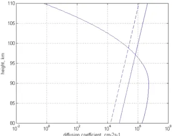
The turbopause region is characterized by transition from the mean molecular mass, constant with altitude, to the mean mass dependent on altitude. The former is provided by eddy turbulence, and the latter is induced by molecular diffusion. A competition between these processes provides the tran-sition from the homosphere to the heterosphere. The tur-bopause altitude can be defined by equalizing the eddy and molecular diffusion coefficients and can be located in the up-per mesosphere or the lower thermosphere. An example of the height distributions of eddy and molecular diffusion co-efficients is shown in Fig. 1.

(2)

432 M. N. Vlasov and M. C. Kelley: Specific features of eddy turbulence in the turbopause region

Fig. 1.Height distributions of molecular diffusion coefficients for Ar and He (dashed and solid lines, respectively) and the eddy diffu-sion coefficient (solid curve).

Although there is progress in estimating the eddy diffu-sion coefficient, significant uncertainty remains in determin-ing the eddy diffusion coefficient. Thus, the experimental data and the theoretical estimates obtained during the period of 1970–1980 included maximum values of the eddy diffu-sion coefficient that were much larger than 1×107cm2s−1 (for example, Justus, 1973; Weinstock, 1984) with a very high peak altitude of 130 km. The minima values were less by two orders of magnitude (Hocking, 1986). Also, very contradictory data on seasonal eddy diffusion varia-tions existed (Blum and Schuchardt, 1978). Later, Vlasov and Korobeynikova (1991) showed that eddy diffusion with a coefficient larger than 5×106cm2s−1 _{induces a} signifi-cant temperature height distribution deviation from empirical model distributions in the lower thermosphere. It was recog-nized that maximum values of the eddy diffusion coefficient occur during summer and at high latitudes. This significant advance was achieved due to the measurements of Fukao et al. (1994) and Lübken (1997), and we have used Lübken’s measurements in this paper. More recent data on the eddy diffusion coefficient are discussed below.

In contrast to the statistical concept of the turbopause lo-calized within the altitude range of 90–110 km, we consider the turbopause as the region where, at any given time, the combination of turbulence and molecular diffusion can be complicated. For example, this is demonstrated by the ap-pearance of long-lived meteor trails, as presented by Kelley at al. (2003). Also, the Turbulent Oxygen Mixing Experiment (TOMEX) (Bishop et al., 2004) showed that “unstable re-gions are well mixed, but the intermediate rere-gions, in some cases, have very small energy dissipation rates”. According to these results, eddy diffusion may be important at altitudes above the turbopause, located at 103 km.

We must emphasize that the energy deposition rates and the eddy diffusion coefficient, Ked, corresponding to the rates estimated in TOMEX (see Tables 1 and 2 in Bishop et al., 2004), are larger than the parameters estimated by Lübken (1997) by a factor of 4–8, and the Ked maximum value is larger than 1×107cm2s−1_{. However, the energy} de-position rate, estimated from the density fluctuation measure-ments carried out during the rocket experiment (Szewczyk et al., 2013), is larger by a factor of 20 than the value estimated by Lübken (1997). We will discuss these results in Sect. 4.

All of the experimental methods have limitations and re-quire some theoretical assumptions. The main assumption is linear dependence of the eddy diffusion coefficient Ked on the energy dissipation rate. Problems with applying this fairly restrictive assumption were noted many times (for ex-ample, Lübken, 1997; Fritts and Luo, 1995; Hocking, 1999). The energy dissipation rate,ε, is a key parameter in deter-mining the eddy diffusion coefficient,Ked, from experimen-tal data. Usually, the spectrum of density fluctuations calcu-lated from experimental data is approximated using the the-oretical model of Heisenberg (1948) and the inner scale,l0, is determined. This parameter is related to the Kolmogorov microscale,η, through the relationl0=9.9η(Lübken et al., 1993). The Kolmogorov microscale is a rough estimate of the size of the smallest eddies, which can provide the turbu-lent energy dissipation by viscosityν. Then theεvalue can be calculated using the formulaε=ν3η−4_{. According to this} formula, theεvalue strongly depends on theηvalue, which is estimated by a rough approximation. For example, let us estimate the impact ofηvalues on the energy dissipation rate using the l0 values inferred from the experimental data by Kelley et al. (2003). These values are changed from 156 m to 222 m, and theεvalue can change from 0.14 W kg−1 _to 0.58 W kg−1_{. The formula}_K

ed=bε/ω2B(∗)is used, and here bis usually assumed to be constant andωBis the buoyancy frequency. Kelley et al. (2003) estimated the Ked-averaged value to be 500 m2s−1_{. Taking into account the}_ε _variation estimated above, theKedvalues can vary from 250 m2s−1to 1000 m2s−1_{, which, except for the very highest values,} cor-respond to measuredKedvalues in the mesosphere and lower thermosphere (Fukao et al., 1994).

(3)

The other uncertainty results from determining thebvalue in formula(∗). Usually,b=0.81 is used (Weinstock, 1978). However, formulaKedωB2(P−Ri) /Ri=ε whereP andRi are the Prandtl and Richardson numbers, respectively, should be used according to Gordiets et al. (1982). The Prandtl num-ber is equal to 1 for uniform turbulence andRi=0.44 forb=

0.81. The Kelvin–Helmholtz instability requires Ri≤0.25, corresponding tob=0.3.

Using the electron density fluctuation spectra obtained by rocket-borne measurements of electron density at low lati-tudes, Das et al. (2009) showed that turbulence is not present continuously in the mesosphere but exists in layers of 100– 200 m interspersed with regions of stability.

Gravity waves, winds, and turbulence are the main dy-namic processes in the upper mesosphere and the lower ther-mosphere (MLT). The source of these processes is uncer-tain, as is their role in the MLT energy budget. For example, Lübken et al. (1993) conclude that the impact of turbulence on the energy budget of the mesosphere and lower thermo-sphere is small. However, Lübken (1997) reconsidered their results and reported the importance of turbulence.

Gravity waves were first suggested by Hines (1960) to ex-plain observed features in MLT. Then, the important role of gravity waves in the circulation, thermal balance, and constituent structures was recognized. Reviews of the work on gravity waves are given by Fritts (1984) and Fritts and Alexander (2003).

Gravity waves can transfer their energy and momentum into the MLT due to their dissipation via nonlinear interac-tion and wave-breaking processes (Weinstock, 1976). The turbulence can be generated in MLT (Lindzen, 1967; Hodges Jr., 1969). Heating can result from this dissipation (Becker, 2004; Medvedev and Klassen, 2003). Also, a downward heat flux can be induced during this dissipation, resulting in cool-ing. Medvedev and Klassen (1995, 2003) considered gravity wave dissipation due to nonlinear interaction across the wave spectrum and showed that there is cooling for saturated grav-ity waves in the upper portion of the MLT. However, there is a problem with estimating these effects, as described next.

It is assumed that the mean atmosphere is expected to be stable, both statically and dynamically, even in the presence of tides (Hodges Jr., 1967; Gardner et al., 2002). However, in the mesopause region where gravity waves can achieve high amplitudes, the combined effect of the background tempera-ture profile, tides, and gravity waves can induce significantly large vertical shears in the horizontal wind and temperature profiles so that the atmosphere becomes unstable and the waves began to dissipate. Note that all of the experimental data on the height distribution of chemical inert gases show mixing of these gases at all altitudes below the mesopause.

It is assumed that eddy turbulence is due to convective or dynamic instability. The former develops when the negative temperature gradient is higher than the adiabatic lapse, and the latter occurs when the dynamic Richardson number,Ri, is less than 0.25. The Richardson number is defined by the

ratio Ri=ω

2 B

S2, (1)

whereωBis the buoyancy frequency given by the formula ω2_B= g

T _∂T ∂z + g Cp , (2)

whereT is the temperature,gis the gravity acceleration,Cp is the heat capacity of air at constant pressure, and

S= " ∂u ∂z 2 + _∂v ∂z

2#1/2

(3)

is the total vertical shear of the horizontal wind with zonal, u, and meridional,v, components.

In general, turbulence can be generated due to gravity waves, produced in the lower atmosphere, traveling upward and breaking at mesospheric heights and/or due to Kelvin– Helmholtz instability, which occurs in situ in the presence of strong wind shears. However, very intense shears would be required to meet the criterionRi< 0.25 in the turbopause region. Also, the strong wind source is not clear.

The time of eddy diffusion can be estimated by the formula τ=H2/Ked=3.6×1011/5×106=7.2×104s≈1 day, meaning that significant fluctuations can exist within this time. Thus, fluctuations with a gradient scale of less than 2 km can take place during 2.2 h. However, rocket measure-ments of the ratio [Ar] / [N2] show the continuity transition from the ratio corresponding to mixing (independent of altitude) to the altitude-dependent ratio corresponding to the diffusive separation of gases with different masses. Note that different experimental data show the mixing of atmospheric constituents below 80 km where conditions for the Kelvin–Helmholtz instability are not met because of low wind shear and high Brunt–Väisälä frequencies.

(4)

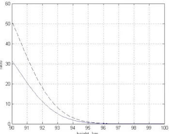
Fig. 2.Height profile of the [Ar] / [N2] ratio in summer solstice at a

latitude of 40◦_{N at 14:00 LT, given by the MSIS-E-90 model.}

than normal cooling corresponding to temperatures given by the MSIS model at altitudes around the turbopause. This phe-nomenon results from strong cooling by eddy turbulence cor-responding to a strong decrease in the eddy diffusion coeffi-cient in the turbopause region (see Fig. 1). This high cool-ing means that the eddy heat transport coefficient should be smaller than the eddy diffusion coefficient.

The goal of this paper is to study the specific features of eddy turbulence in transition from the homosphere to the het-erosphere under different geophysical conditions. Also, we analyze the conditions for developing eddy turbulence in the small temperature gradient region and below the main wind shear layer because, according to our results, the eddy tur-bulence peak occurs below the wind shear maximum and in regions with a positive or small negative temperature gradi-ent.

In Sect. 2 we infer the height profile of the eddy diffusion coefficients using continuity equations and the height profiles of the chemical inert gases given by the MSIS-E-90 model. In Sect. 3 we estimate the cooling/heating profiles correspond-ing to the eddy heat transport coefficients equaled to the eddy diffusion coefficients estimated in Sect. 2. In Sect. 4, using the results obtained in previous sections and the eddy dif-fusion coefficients inferred from experimental data (Lübken, 1997; Bishop et al., 2004), we determine the specific features of eddy turbulence in the turbopause region and consider an instability mechanism in this region.

2 Estimate of the eddy diffusion coefficient from height distributions of chemical inert gases given by the MSIS-E-90 model

The [Ar] / [N2] ratio measured in rocket-borne measure-ments is widely used to determine the turbopause altitude

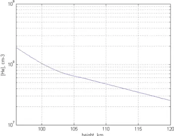
Fig. 3.[He] height profiles according to the MSIS-E-90 model: win-ter solstice at 40◦N latitude at 14:00 LT (dashed curve), summer solstice at 40◦_{N latitude at 14:00 LT (solid curve), the summer} sol-stice at the equator at the same local time (dashed-dotted curve), and polar summer solstice at 70◦_{N latitude (dotted curve), the} lon-gitude of 0◦_{for all data. All eddy diffusion coefficients are inferred} from the MSIS-E-90 data, and the cooling rates corresponding to these coefficients are presented for the above given condition.

(von Zahn et al., 1990). An example of this ratio correspond-ing to the MSIS-E-90 data is shown in Fig. 2. In this case, the turbopause altitude of 90–92 km corresponds to the transition from an almost constant ratio to a significantly changed ratio. Changes in the helium height distribution are largest in the transition region from the homosphere to the heterosphere. As seen from Fig. 3, these distributions differ at different lat-itudes and in different seasons. The steepest gradient of the [He] distribution corresponds to the largest eddy diffusion coefficient. This means that the eddy diffusion coefficient in summer should be larger than during winter at middle and high latitudes, and the maximum value of this coefficient should occur during polar summer. This qualitative estimate is in agreement with experimental turbulence data observed by a variety of techniques (see, for example, Hocking, 1986; Fukao et al., 1994; Lübken, 1997; Kelley et al., 2003).

The continuity equation for the chemical inert constituents is

∂ ∂z

−Di

_∂n

∂z+ n HHe

+(1+αT) n T

∂T ∂z

+ ∂

∂z

−Ked

_∂n

∂z+ n H+

n T

∂T ∂z

(5)

Fig. 4.Height profile of the eddy diffusion coefficient correspond-ing to the [He] height distribution shown by the dashed curve in Fig. 5a.

D=

P

i

AiTsini/N

N ,

where Ai and si correspond to values for helium diffu-sion in N2, O2, and O given in Table 15.1 in Banks and Kockarts (1973), andniandNare the densities of these con-stituents and the total density, respectively. The altitude pro-file ofKedis given by the widely used approximation sug-gested by Shimazaki (1971):

Ked=Kedmexp

h

−s (z−zm)2

i

z > zm, (5) wheresis the reciprocal of the scale heights,zmis the height of theKedpeak, andK_edmis the value of the peak. Note that Eq. (4) requires similar eddy and molecular diffusion, which means that the eddy scales must be much larger than the free pass of neutrals and much smaller than the scale height of the atmosphere.

Using the numerical solution of Eq. (4) and data on the densities and temperature given by the MSIS-E-90 model, it is possible to estimate the eddy diffusion coefficient in the region of the transition from the homosphere to the hetero-sphere. The [Ar] / [N2] height profiles are also used to esti-mate the turbopause altitudes. The example of the height dis-tribution of the eddy diffusion coefficient inferred using this approach is shown in Fig. 4.

Note that Eq. (4) does not include the term with vertical transport. The excellent agreement between the [He] height heterospheric profile at altitudes significantly higher than the turbopause altitude calculated by Eq. (4) and the [He] height profile given by the MSIS-E-90 model shows that the [He] distributions correspond exactly to the barometric law.

As seen from Fig. 5a, the [He] height profile calculated by Eq. (4) with theKedprofile shown in Fig. 4 is in good agreement with the [He] distribution given by the MSIS-E-90 model. The same agreement exists in other cases (for ex-ample, see Fig. 5d), meaning that the eddy diffusion coef-ficients inferred using the [He] height distributions and the [Ar] / [N2] distributions are correct and can be used to further our study. The seasonal and latitudinal variations of the eddy diffusion coefficient estimated by this method are in good agreement with generally recognized variations, as seen from theKedvalues given in the captions to Fig. 5a, b, and d. Also, these variations coincide with the qualitative estimate corre-sponding to the [He] variations, as mentioned in the second paragraph of this section.

3 Heating and cooling induced by eddy turbulence corresponding to the eddy diffusion coefficients inferred from MSIS-E-90 data

The eddy turbulence heating/cooling rate is given by equa-tion (Vlasov and Kelley, 2010)

Qed= ∂

∂z

KehCpρ

_∂T

∂z + g

Cp

+Kehρ g T c

_∂T

∂z + g Cp

, (6)

whereKehis the coefficient of eddy heat transport,ρ is the undisturbed gas density,g is the gravitational acceleration, T is the temperature,Cpis the specific heat at constant pres-sure, andcis a dimensionless constant commonly taken to be 0.8. The vertical energy flux is given by the formula (A07) F2= −ρCp5Kec

∂2

∂z (7)

or the formula (BM09) F2= −Keh

∂2

∂z, (8)

where2=T /5is the potential temperature. As seen from the formula given below, the flux given by Akmaev is the same as the flux in the eddy heating rate term in Eq. (6), F2= −ρCp5Kec

∂2

∂z = −ρCpKeh

_∂T

∂z + g Cp

, (9)

which corresponds to the flux in the fourth term on the right-hand side of Eq. (11) in BM09 and also corresponds to the flux in theµterm without molecular diffusion but with an “eddy diffusion coefficient from the GW parameterization and vertical diffusion scheme”. The first term in Eq. (10) in BM09 can be presented asKehω_b2because

̟_B2=g

1 2

∂2 ∂z

(6)

Fig. 5a.[He] height profiles in winter solstice given by the MSIS-E-90 model (solid curve) and calculated (dashed curve) with the eddy diffusion coefficient shown in Fig. 4 (K_edm=3×106cm2s−1_, zm=95 km,s=0.01 km−2).

Fig. 5b.The same as in Fig. 5a but in summer solstice withK_edm=

6×106cm2s−1_,_z

m=92 km, ands=0.01 km−2_.

This term is similar to the second term in our Eq. (6), but our term includes the coefficientcdetermined by the ratio of the Richardson number,Ri=̟_B2/(∂u/∂z)2, to the turbulent Prandtl number,P =Kem/Keh, for the steady mean motion (Kem is the eddy momentum transport coefficient). Chang-ing the cvalue, we take into account the effect of gravity waves. Thus, the second term in our Eq. (6) includes the first term of Eq. (10) and theεmterm in Eq. (11) (BM09). Ex-cluding theεGWterm, we see that our Eq. (6) accumulates the terms of Eq. (11) but with different eddy diffusion coef-ficients. Thus, the formulas for the eddy heating/cooling rate coincide with formulas for these rates that were obtained and

Fig. 5c.The same as in Fig. 5a but at the equator.

Fig. 5d.[He] height profile given by the MSIS-E-90 model in the polar region (solid line) and calculated by Eq. (4) withK_edm=7×

106cm2s−1_,_z

m=84 km, ands=0.01 km−2_{(dashed curve).}

used in estimating the thermal effect of gravity waves (A07, BM09). This means that heating/cooling by gravity waves can be described by eddy turbulence heat transport. The dis-cussion above shows that the impact of gravity waves on ther-mal balance can be described by eddy heat transport.

(7)

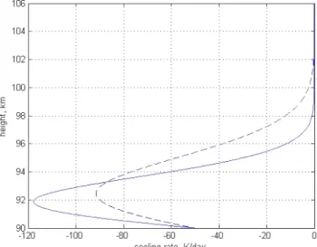
Fig. 6a.Height profile of the cooling rate in winter solstice calcu-lated with the coefficient of eddy heat transport equaled to the eddy diffusion coefficient shown in Fig. 2.

Fig. 6b.Height profiles of the cooling rate calculated withK_eh= Kedinferred from the [He] distribution in summer solstice (Kedm=

5×106cm2s−1_,_s₌₀_._{01 km}−2_,_c₌₀_._8,_P ₌_1).

4 Uniform, localized, and large-scale turbulence

Uniform turbulence is characterized by a wide spectrum of eddy scales, from scales much larger than the free path to scales much smaller than the atmospheric scale height. In this case, the eddy momentum and heat transport coefficients are equal and the Prandtl numberP equals 1. However, more complex turbulence can take place. Observations of artificial clouds and meteor trails show that turbulence is very inter-mittent, both temporarily and spatially (Kelley et al., 2003; Bishop et al., 2004). The thin turbulent layers separated by regions of very weak turbulence or laminar flow occur. An ensemble of gravity waves can produce turbulent layers with

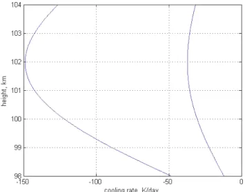
Fig. 6c.Height profile of the cooling rate calculated withK_eh= Ked inferred from the [He] distribution at the summer equator

(Km=3×106cm2s−1_,_s₌₀_._{02 km}−2_,_Ri_{= 0.8).}

Fig. 6d.Height profiles of the cooling rate calculated withK_eh= Ked inferred from the [He] distribution at polar summer solstice

(K_edm=5×106cm2s−1_, _s₌₀_._{002 km}−2_, _c₌₀_._4, _P₌_2, _z m=

84 km).

a thickness of a few tens of meters to a kilometer. This prob-lem was discussed by Hocking (1999). Observations of artifi-cial clouds and meteor trails show that turbulence is very in-termittent, both temporarily and spatially (Kelley et al., 2003; Bishop et al., 2004). In this case, the average eddy diffu-sion and eddy heat transport coefficients can differ, and the Prandtl number can exceed 1 and may be up to 3 (Fritts and Dunkerton, 1985). The Prandtl number is determined by the ratio

(8)

Fig. 7a. Height distributions of the thermal conductivity (solid curve) and eddy heat conductivity (dashed curve) with the eddy heat transport coefficient equaled toKed, shown in Fig. 4. Eddy heat

conductivity is given by the formulaλed=KecCpρerg (cm s K)−1, and the thermal heat conductivity is given by the formula λ_th=38.2T0.69+1.9T+51.4 erg (cm s K)−1_{(Banks and Kockarts,}

1973).

Fig. 7b.Ratio of the eddy diffusion and molecular diffusion coeffi-cients (dashed curve) and the ratio of eddy heat conductivity to the thermal conductivity (solid curve) calculated with the eddy diffu-sion coefficient given by L97 for polar summer.

where µ is the dynamic viscosity and λ is the thermal conductivity. Using the values of these parameters (µ=3.8×10−6_T0.69_{g cm}−1_s−1_, _λ₌ 38.2×T0.69+1.9T +51.4 erg cm−1_s−1_K−1₎ _given _by Banks and Kockarts (1973),P=0.47 can be found for N2 andT =200 K. The relation

P =Ked/Keh (11)

Fig. 8.Temperature height profiles in winter (dashed curve) and summer solstices (solid curve) at middle latitudes, at the equator (dashed-dotted curve), and at high latitudes (dotted curve), as given by the MSIS-E-90 model.

can be obtained for eddy turbulence because, in this case, µ∝Kedρ andλ∝KehρCp. Obviously, eddy turbulence in-creases the viscosity. If we assume that the gravity wave energy dissipates to wind shear in the turbopause region, we could use the formulaKem=0.81ε/ω2_B(Fritts and Luo, 1995). This formula is the same as the formula used forKed (Fritts and Luo, 1995; Lübek, 1997), and Eq. (11) can be applied because P =Kem/Keh. As seen from Fig. 7a, the eddy heat conductivity can be much higher than the molecu-lar thermal conductivity in spite of the molecu-large Prandtl number. The ratios of the eddy diffusion coefficient to the molecu-lar diffusion coefficient and the eddy heat conductivity to the thermal conductivity are large at theKedpeak altitude, as can be seen from Fig. 7b.

Analysis of Eq. (6) shows that the negative vertical gradi-ent of the eddy heat transport coefficigradi-ent is the main cause of the cooling. This gradient is located in the turbopause region, and the turbopause altitude depends on this gradient.

Note that, according to the MSIS-E-90 data, conditions for developing Kelvin–Helmholtz instabilities in the turbopause region do not exist because the Richardson number is larger than 0.25 and the temperature gradient is positive or close to zero (see Fig. 8). However, these data presented average conditions. In the real atmosphere, there are significant fluc-tuations corresponding to turbulence that provide mixing of the atmospheric constituents.

(9)

Fig. 9.Height profile of the eddy diffusion coefficient measured by Lübken (1997) in the polar region (solid curve) and approx-imated by Eq. (5) (dashed curve) with parametersK_edm=1.83×

106cm2s−1andzm=90 km, shown by the horizontal line.

is given by the relation

Re=ρU L/µ, (12)

whereUis the velocity,Lis the characteristic pipe diameter, andµ=3.8×10−6_T0.69_{g cm}−1_s−1_{is the dynamic} viscos-ity for the mixture of N2and O2(Bank and Kockarts, 1973). For example, using densityρ=6×10−10_{g cm}−3_and tem-peratureT =180 K at 100 km as given by the MSIS-E-90 model, the velocity ρ=6×10−10_{g cm}−3 _{and temperature} T =180 K at 100 km given by the MSIS-E-90 model, and the velocityU=50 m s−1_{corresponding to}_U_{for the mean} wind at 100 km withL=1 km, a Reynolds number of 2300 can be found. Turbulence can develop when the Reynolds number exceeds 1000. In this case, localized instabilities can occur. However, a problem exists with the thin turbu-lent layer boundary conditions, and applying this approach to free atmospheric gas may be a questionable assumption. Note that low Richardson numbers ofRi< 0.25 are possible in the narrow range of altitudes around 100 km where strong wind shear occurs, according to Larsen (2002). However, these low numbers simultaneously need the lowωBvalue that large negative temperature gradients can provide. According to MSIS-E-90 data, however, the temperature gradient is very small in the turbopause region.

Let us compare the cooling rate calculated with the eddy diffusion coefficient estimated by Lübken (1997, hereafter referred to as L97) and shown in Fig. 10 and the cooling rate shown in Fig. 6d. Both rates correspond to the polar summer. As seen from the cooling rates shown in Figs. 6d and 10, the maximum cooling rate corresponding to theKed of L97 is larger than the maximum rate shown in Fig. 6d, but theK_edm values of the latter are less by a factor of 2.5 than theK_edm

Fig. 10. Height profiles of the cooling rate (solid curve) calcu-lated with the eddy diffusion coefficient shown by a dashed curve (s=0.1 km−2₎_{in Fig. 9 and calculated with}_s₌₀_._{03 km}−2

corre-sponding to agreement with the cooling rate induced by the eddy diffusion coefficient shown in Fig. 9 below the Ked peak. The

straight line shows this peak.

of L97. This result shows a very important role of theKed gradient above the peak characterized by thesvalue, which is much larger for theKedprofile given by L97 (see Fig. 9).

The very important role of theKedgradient above the peak can be seen by analyzing the thermal equation. This equation can be written as

KehCp ∂2T

∂z2 +Cp

_∂K

eh ∂z −

Keh H

_∂T

∂z +g

_∂K

eh ∂z −

Keh H

+ε+q−L=0, (13) which includesQehgiven by Eq. (6), heating due to the en-ergy dissipation of gravity waves, ε, chemical heating and heating by the ultraviolet solar radiation,q, and cooling by the CO2and O infrared radiation,L. According to the con-ditions (L97), theKedpeak is in the mesopause and Eq. (13) can be simplified to the relation

K_ehmg/H=q+ε−L. (14)

Using this relation with the ε value given in Table 3 in Lübken (1997) at the Ked peak altitude and (q−L)≤ 10 K day−1_{, the} _Km

eh value can be found to be ≤1.1× 106_cm2_s−1_{. This value is significantly less than} _Km

(10)

Fig. 11.Cooling rates calculated with the eddy diffusion shown in Fig. 3 in Hecht et al. (2004) (curve with the peak value of

−37 K day−1_{) and with the eddy diffusion coefficient with}_Km ed=

1×107cm2s−1_{(curve with the peak value of}₋_{150 K day}−1₎

cor-responding to the values given in Table 2 in Bishop et al. (2004).

Lübken is very large. In this case, thePvalue was larger than 2, indicating localized turbulence.

Following L97 and using the formulas given by Weinstock (1978, 1981), we obtain the formula

Led=10.46K_eh3/4ε−1/4, (15) whereLedis the outer turbulence scale andεis the turbulent energy dissipation rate. Using theεvalues measured by L97 during the summer and theKed profiles given in Table 3 in L97, it is possible to estimateLed=0.97 km in theKedpeak. This turbulence scale is comparable to the scale height of atmospheric gas and is an indication of localized turbulence. The introduction mentioned that very high eddy diffusion coefficients were estimated in TOMEX using the energy de-position rates inferred from the observed passive tracer trails (Bishop et al., 2004). Also, the eddy diffusion coefficients were inferred from airglow observed during TOMEX (Hecht et al., 2004). The latter were less by a factor of 5–10 than the former. We could not find an explanation for this huge dis-agreement. The cooling rates calculated by Eq. (6) with the Kedheight profile shown in Fig. 3 in Hecht et al. (2004) and the same profile but normalized byK_edm=1×107cm2s−1_are shown in Fig. 11. The cooling rate calculated with the low eddy diffusion coefficient corresponds to the normal cool-ing rates, but the coolcool-ing rate with a high eddy diffusion co-efficient is very high and we must assume that the Prandtl number is 3 in this case. We assume that the rate coefficients inferred from a chemical release by Bishop et al. (2004) are overestimated.

In the introduction, we also mentioned the very large energy deposition rate of ε=2 W kg−1_{= 200 K day}−1_,

estimated by Szewczyk et al. (2013) based on the results of their rocket experiment to measure density fluctuations. The maximum value of the eddy diffusion coefficient for the peak of the smoothed energy dissipation rate shown in Fig. 1b (green curve) in Szewczyk et al. (2013) and theω2_B value corresponding to the temperature height profile within the altitude range of 89–92 km shown in Fig. 1a (black curve) in Szewczyk et al. (2013) can be found to be 7.5×107cm2s−1_. ThisK_edmvalue is higher by a factor of about 3 than the value estimated by Bishop et al. (2004). In this case, the cooling rates above the K_edm peak are much higher than the cool-ing rates calculated for the K_edm peak given by Bishop et al. (2004) and shown in Fig. 11. Assuming a large Prandtl number, it is possible to decrease theKehvalue and cooling rate. However, the Ked value is very high, and the impact of eddy diffusion on neutral composition is very strong. For example, very low atomic density can be found (Vlasov and Kelley, 2010), contradicting all of the experimental data gen-eralized by the MSIS-E-90 model. Taking this effect into ac-count, this very high energy deposition rate can be assumed to occur for 1 h but no longer. Note that the observed inver-sion layers (double mesopause) are usually characterized by small gradients and the temperature enhancements (Yu and She, 1995). A heating rate of about 30–40 K day−1_can pro-vide these temperature enhancements (Vlasov and Kelley, 2012). For example, note that the normal heating rate at 90 km does not exceed 10 K day−1_{(Roble, 1995).}

We plan to analyze methods for estimating eddy diffusion coefficients, based on density fluctuation measurements and passive tracer trails, in the near feature.

5 Conclusions

Using the continuity equation and the [He], [Ar], and [N2] height distributions and other parameters given by the MSIS-E-90 model, the eddy diffusion coefficients are estimated for the turbopause region. The latitudinal and seasonal variations of the eddy diffusion coefficients inferred from the chemical inert constituent distributions given by the MSIS-E-90 model are in good agreement with observations of these variations. The cooling rates calculated with the eddy heat transport coefficients equaled to the eddy diffusion coefficients are found to be much larger than the normal cooling rates cor-responding to temperatures given by the MSIS-E-90 model. In this case, the eddy heat transport coefficient should de-crease by a factor of 2 and above, and the Prandtl number may be 2 or larger. Also, very strong cooling is estimated for the eddy diffusion coefficients inferred from the experimen-tal data, meaning that localized turbulence should exist in the turbopause region.

(11)

decrease this gradient because, in this case, the turbopause altitude can be found at altitudes above 110–115 km, contra-dicting the MSIS-E-90 model and other experimental data.

There are no conditions for developing dynamic or con-vective instability in the turbopause region because of the high buoyancy frequency value ω_B2≈4.5×10−4_s−1_. We consider the average condition corresponding to the MSIS-E-90 model, which means that the average value of the wind shear can be used. The value does not exceed 20 m−1_s−1_km−1 _{(Larsen, 2002), and the}_Ri_{value is about} 1. We suggest that the criterion for developing localized tur-bulence may differ from the usual criterion and that local-ized turbulence may develop as a result of strong wind with a mean wind shear in the narrow layers of turbulence, lim-ited by boundaries with undisturbed gas. In this case, the gas transport inside a turbulent layer may be compared to flow in a narrow pipe. In any case, the development of localized turbulence in the turbopause region needs further study.

The existence of localized turbulence in the turbopause re-gion is important in understanding the effect of eddy turbu-lence on thermal balance in the MLT. We conclude that a new approach for the parameterization of energy deposition by gravity waves is needed. It must be emphasized that the localized turbulence is found by using the data given by the MSIS-E-90 model corresponding to the averaged conditions. Thus, our knowledge of the mean thermal structure in the transition region from the homosphere to the heterosphere will improve due to a better understanding of the specific fea-tures of mean dynamic forcing.

Acknowledgements. Work at Cornell was supported by the National

Science Foundation under grant ATM-0551107.

Topical Editor C. Jacobi thanks two anonymous referees for their help in evaluating this paper.

References

Akmaev, R. A.: On the energetics of mean-flow interactions with thermally dissipating gravity waves, J. Geophys. Res., 112, D11125, doi:10.1029/2006JD007908, 2007.

Banks, P. M. and Kockarts, G.: Aeronomy, part B, Academic Press, New York, 11–12, 1973.

Becker, E.: Direct heating rates associated with gravity wave satu-ration, J. Atmos. Sol.-Terr., 66, 683–696, 2004.

Becker, E. and McLandress, C.: Consistent scale interaction of grav-ity waves in the Doppler spread parameterization, J. Atmos. Sci., 66, 1434–1449, 2009.

Bishop, R. L., Larsen, M. F., Hecht, J. H., Liu, A. Z., and Gard-ner, C. S.: TOMEX: Mesospheric and lower thermospheric dif-fusivity and instability layers, J. Geophys. Res., 109, D02S03, doi:10.1029/2002JD003079, 2004.

Blum, P. W. and Schuchardt, K. G. H.: Semi-theoretical global mod-els of the eddy diffusion coefficient based on satellite data, J. At-mos. Terr. Phys., 40, 1137–1142, 1978.

Das, U., Sinha, H. S. S., Sharma, S., Chandra, H., and Das, S. K.: Fine structure of the low-latitude mesospheric turbulence, J. Geo-phys. Res., 114, D10111, doi:10.1029/2008JD011307, 2009. Fritts, D. C.: Gravity wave saturation in the middle atmosphere: A

review of theory and observations, Rev. Geophys., 82, 275–308, 1984.

Fritts, D. C. and Alexander, M. J.: Gravity wave dynamics and effects in the middle atmosphere, Rev. Geophys., 41, 1003, doi:10.1029/2001RG000106, 2003.

Fritts, D. C. and Dunkerton, T. J.: Fluxes of heat and constituents due to convective unstable gravity waves, J. Amos. Sci., 42, 549– 556, 1985.

Fritts, D. C. and Luo, Z.: Dynamical and radiative forcing of the summer mesopause circulation and thermal structure, J. Geo-phys. Res., 100, 3119–3128, 1995.

Fukao, S., Yamanaka, M. D., Ao, N., Hocking, W. K., Sato, T., Ya-mamoto, M., Nakamura, T., Tsuda, T., and Kato, S.: Seasonal variability of vertical eddy diffusivity in the middle atmosphere, 1. Three-year observations by the middle and upper atmosphere radar, J. Geophys. Res., 99, 18973–18987, 1994.

Gardner, C. S., Zhao, Y., and Liu, A. Z.: Atmospheric stability and gravity wave dissipation in the mesopause region, J. Atmos. Sol.-Terr., 64, 923–929, 2002.

Gordiets, B. F., Kulikov, Yu. N., Markov, M. N., and Marov, M. Ya.: Numerical modeling of the thermospheric heat budget, J. Geophys. Res., 87, 4504–4514, 1982.

Hecht, J. H., Liu, A. Z., Walterscheid, R. L., Roble, R. G., Larsen, M. F., and Clemmons, J. H.: Airglow emissions and oxygen mixing ratios from the photometer experiment on the Turbulent Oxygen Mixing Experiment (TOMEX), J. Geophys. Res., 109, D02S05, doi:10.1029/2002JD003035, 2004.

Hedin, A. E.: Extension of the MSIS thermosphere model into the middle and lower atmosphere, J. Geophys. Res., 96, 1159–1172, 1991.

Heisenberg, W.: Zur statistichen Theorie der Turbulentz, Z. Phys., 124, 628–657, 1948.

Hines, C. O.: Internal atmospheric gravity waves at ionospheric heights, Can. J. Phys., 38, 1441–1481, 1960.

Hocking, W. K.: Observation and measurement of turbulence in the middle atmosphere with a VHF radar, J. Atmos. Terr. Phys., 48, 655–670, 1986.

Hocking, W. K.: The dynamical parameters of turbulence theory as they apply to middle atmosphere studies, Earth Planet Space, 51, 525–541, 1999.

Hodges Jr., R. R.: Generation of turbulence in the upper atmo-sphere by internal gravity waves, J. Geophys. Res., 72, 3455– 3458, 1967.

Hodges Jr., R. R.: Eddy diffusion coefficients due to instabilities in internal gravity waves, J. Geophys. Res., 74, 4087–4090, 1969. Justus, C. G.: Upper atmospheric mixing by gravity waves,

Proceed-ings of the AIAA/AMS International Conference on the Environ-mental Impact of Aerospace Operations in the High Atmosphere, paper No. 73–495, Denver, CO, June 11–13, 1973.

Kelley, M. C., Kruschwitz, C. A., Gardner, C. S., Drummond, J. D., and Kane, T. J.: Mesospheric turbulence measurements from persistent Leonid meteor train observations, J. Geophys. Res., 108, 8454, doi:10.1029/2002JD002392, 2003.

(12)

wind measurements, J. Geophys. Res., 107, SIA28.1–SIA28.14, doi:10.1029/2001JA000218, 2002.

Lindzen, R. S.: Thermally driven diurnal tide in the atmosphere, Q. J. Roy. Meteorol. Soc., 93, 18–42, 1967.

Lübken, F. J.: Seasonal variation of turbulent energy dissipation rates at high latitudes as determined by in situ measurements of neutral density fluctuations, J. Geophys. Res., 102, 13441– 13456, 1997.

Lübken, F. J., Hillert, W., Lehmacher, G., and von Zahn, U.: Experi-ments revealing small impact of turbulence on the energy budget of the mesosphere and lower thermosphere, J. Geophys. Res., 98, 20369–20384, 1993.

Medvedev, A. S. and Klaassen, G. P.: Vertical evolution of gravity wave spectra and the parameterization of associated wave drag, J. Geophys. Res., 100, 25841–25853, 1995.

Medvedev, A. S. and Klaassen, G. P.: Thermal effects of saturating gravity waves in the atmosphere, J. Geophys. Res., 108, 4040, doi:10.1029/2002JD002504, 2003.

Rees, D., Roper, R. G., Lloyd, K. H., and Low, C. H.: Determination of the structure of the atmosphere between 90 and 250 km by means of contaminant releases at Woomera, May 1968, Philos. T. Roy. Soc. London A, 271, 631–663, 1972.

Roble, R. G.: Energetics of the mesosphere and thermosphere, Geo-phys. Monogr., 87, 1–21, 1995.

Shimazaki, T.: Effective eddy diffusion coefficient and atmospheric composition in the lower thermosphere, J. Atmos. Terr. Phys., 33, 1383–1401, 1971.

Szewczyk, A., Strelnikov, B., Rapp, M., Strelnikova, I., Baum-garten, G., Kaifler, N., Dunker, T., and Hoppe, U.-P.: Simulta-neous observations of a Mesospheric Inversion Layer and tur-bulence during the ECOMA-2010 rocket campaign, Ann. Geo-phys., 31, 775–785, doi:10.5194/angeo-31-775-2013, 2013.

Vlasov, M. N. and Kelley, M. C.: Estimates of eddy turbulence con-sistent with seasonal variations of atomic oxygen and its possible role in the seasonal cycle of mesopause temperature, Ann. Geo-phys., 28, 2103–2110, doi:10.5194/angeo-28-2103-2010, 2010. Vlasov, M. N. and Kelley, M. C.: Eddy turbulence, the double

mesopause, and the double layer of atomic oxygen, Ann. Geo-phys., 30, 251–258, doi:10.5194/angeo-30-251-2012, 2012. Vlasov, M. N. and Korobeynikova, T. V.: Effect of the turbulence,

infrared radiation and mass-averaged transport on the height dis-tribution of temperature in the middle-latitude and high latitude thermosphere, Cosmic Res., 29, 469–474, 1991.

von Zahn, U., Lübken, F.-J., and Pfitz, C.: BUGATTI experiments: Mass spectrometric studies of lower thermosphere eddy mixing and turbulence, J. Geophys. Res., 95, 7443–7465, 1990. Weinstock, J.: Nonlinear theory of acoustic-gravity waves, 1,

Sat-uration and enhanced diffusion, J. Geophys. Res., 81, 633–652, 1976.

Weinstock, J.: Vertical turbulent diffusion in a stably stratified fluid, J. Atmos. Sci., 35, 1022–1027, 1978.

Weinstock, J.: Energy dissipation rates of turbulence in the stable free atmosphere, J. Atmos. Sci., 38, 880–883, 1981.