Abstract
This paper focuses on a metamodel-based design optimization algorithm. The intention is to improve its computational cost and convergence rate. Metamodel-based optimization method intro-duced here, provides the necessary means to reduce the computa-tional cost and convergence rate of the optimization through a surrogate. This algorithm is a combination of a high quality approx-imation technique called Inverse Distance Weighting and a meta-heuristic algorithm called Harmony Search. The outcome is then polished by a semi-tabu search algorithm. This algorithm adopts a filtering system and determines solution vectors where exact simu-lation should be applied. The performance of the algorithm is eval-uated by standard truss design problems and there has been a significant decrease in the computational effort and improvement of convergence rate.
Keywords
Surrogate-based optimization; Metamodeling; Harmony Search Algorithm; Inverse Distance Weighting model
An improved version of Inverse Distance Weighting
metamodel assisted Harmony Search algorithm for truss
design optimization
1 INTRODUCTION
Employing exact simulations are very common in optimizing engineering design. The problem with some of the most common and robust optimization algorithms such as Genetic Algorithm, Ant Colony, and Harmony Search, is that they entail a large number of iterations for reaching the optimum solution [1-4]. This is a significant barrier when applying exact simulations to real life engineering optimization problems. It has long been recognized that approximations or metamodeling techniques are most effec-tive tools for reducing the computational effort in complex problems. The basic approach is to replace the computationally expensive simulation with a compatible approximate, which is then used in opti-mization runs. This inexact model is often referred to as metamodel (model of a model). A survey on the use of metamodels in structural optimization has been carried out by Barthelemy and Haftka [5] and recently, Jin et al. [6] and Martin and Simpson [7] have reviewed metamodeling techniques for some engineering optimizations.
Notations
Normalization factor
Fitted semi-variance of and
fitted semi-variance between z x( )i and z x( 0)
Y. Gholipour1, M.M. Shahbazi*, 2,
A. Behnia3
1,2:University of Tehran, College of Engineering Engineering Optimization Research Group, Tehran, Iran Tel.: +98-2161112178, Fax: +98-2161112177
3:University Malaya, Civil Engineering Department - Structure and Material
Received 04 Jan 2012 In received form 20 Aug 2012
Material density of each truss member Maximum allowable deflection
Deflection of each truss member
Maximum existing deflection
Maximum allowable stress
Stress of each truss member
Maximum existing stress
Search domain of area of each member Lagrange multiplier
The minimum allowable area of truss member
The maximum allowable area of truss member Cross sectional area of each truss member
Cross sectional area of each truss member generated at new steps
Normalized cross-sectional area of each member
The number of data points included in the circle with radius r Distance between to
Observation point Modulus of elasticity Objective function
HM Harmony memory
HMCR Harmony memory consideration rate
HMS The size of harmony memory
Current iteration number of the algorithm Total number of iterations
Length of each truss member The number of truss members The number of decision variables Total number of data points Test point
PAR Pitch adjusting rate
The minimum number if sample point entries Radius of the circle containing the data points Sample grid matrix
Structure weight Test point
Observation point and optimization variable
The new value of
Set of possible range of each decision variable
The maximum value of kth decision variable The minimum value of kth decision variable random variable to be estimated
The value at the observation point
Optimization using metamodels entails [8]:
1. The exact model is replaced by a low order polynomial. This is to reduce the number of exact simu-lations and smooth out the numerical noise.
2. Enables separation of the analysis code from the optimization routine and eases the integration of codes from various disciplines.
3. Provides an overall view of the design search space.
4. Provides an in depth knowledge of the problem domain and hence makes it easier to adjust im-portant design parameters during the optimization process.
The shortcoming of metamodel, especially those using polynomials for their approximations, is that the cost of providing precise data for fitting the global approximations increases rapidly with the number of design variables, which makes it difficult to construct a good global approximation with low order polynomials.
Some well-known metamodel methods are: Inverse Distance Weighting (IDW) [9]; Polynomial Re-gression (PR) [6, 8]; Moving Least Squares Method (MLSM) [8]; Kriging (KG) [7, 10-14]; Multivariate Adaptive Regression Splines (MARS) [15]; and Radial Basis Function (RBF) [6, 8].
The algorithm presented in this paper is a combination of IDW and HS, which provides a more ro-bust and global search capabilities. An immature version of IDW+HS algorithm has been already pub-lished by the authors [16]. In this research, the prior algorithm is enhanced by normalizing the results and then polishing the final outcome using a semi-tabu search method. IDW is selected for its applica-bility and ease of use for multidimensional metamodeling problems and HS is selected for its aapplica-bility to support continuous variable functions [3, 17-21]. The numerical results shows that the enhanced IDW+HS algorithm (IDW+HS+Tabu), in comparison to the pure HS algorithm as well as the other ventional meta-heuristic algorithms (GA and ACO), leads to a lower computational cost and higher con-vergence rate.
2 APPROXIMATION ALGORITHM SELECTION
As mentioned above, the IDW model is employed in this research for approximation. The easier extend-ibility and competitive computational cost of this model compared to the other interpolation methods such as Kriging (KG), Polynomial Regression (PR), Multivariate Adaptive Regression Splines (MARS), Radial Basis Functions (RBF) caused the IDW to be chosen and employed in this work [6, 22]. The dom-inant problems of these methods are their high computational cost and dimension limit.
One serious problem of the KG, for example, is the large number of observation points needed to es-timate the result [23]. On the other hand, as in the IDW, the kriged eses-timate is a weighted average of the values at the observation points in which the weights are obtained by solving (1).
(1)
where is the fitted semi-variance of and , y is a Lagrange multiplier and
is the fitted semi-variance between and , is the distance from test point to observa-tion point xi, and z is the random variable to be estimated [22]. This weighting formulation signifi-cantly increases the computational effort, while having a small difference in results compared to IDW [24].
The other models involve similar drawbacks. For instance, in spite of the quick convergence [25] and easy implementation of PR [6], some instabilities may arise when applying this technique to highly nonlinear problems with high-order polynomials [6, 26] or it may be too difficult to take sufficient sample data to estimate all of the coefficients in the polynomial equation, particularly in large
sions. MARS, also did not show a satisfying performance when a scarce set of samples is applied [6]. As far as RBF is concerned, although it has performed well in metamodeling problems, when the sample points grow up, the performance of the method decreases [8]. Although a Shepard like modification [9] seems to be applicable for enhancing the performance, it is not considered in this research because of its complexity and high computational effort. On the other hand, the overall accuracy essentially de-pends on the selected basis function for a given set of data samples in the modified versions [27].
In terms of cross-validation, the accuracy of the approximation is not highly important at the early stages. Instead, computational cost must be of a great importance in selecting the approximation meth-od. On the other hand, while the algorithm closes to the final stages, the predicted values are becoming closer to the global optimum (Figure 1).
Figure 1 Closeness of the IDW result to the global optimum 3 INVERSE DISTANCE WEIGHTING MODEL (IDW)
The IDW is a multivariable model based on an interpolation, which is well suited to irregularly spaced data. In two-dimensional space, there are two general types of exact interpolation methods: Single global function and a collection of simple and local functions. The former is usually accompa-nied by an unmanageable complexity, while the latter is well defined and matches appropriately at its boundaries and is continuously differentiable even at the local junctions [9].
The value at any point in a plane is a weighted average of values at the data point in which weighting is a function of distance to those points. Shepard [9] has introduced (2) for interpolating values at . The function indicates that the points further away from will have lower weights.
(2)
where is the value at the data point and is the Cartesian distance between and ( ). As approaches to a data point , approaches to zero. For , both left and right partial derivatives exist and for , there is no derivative. Empirical data shows that the higher exponents ( ) tend to make the surface relatively flat near all data points with very steep
gradi-P Di
P P
i
z Di di P Di
[ , i]
d P D P Di di u = 1
1
u <
2
u >
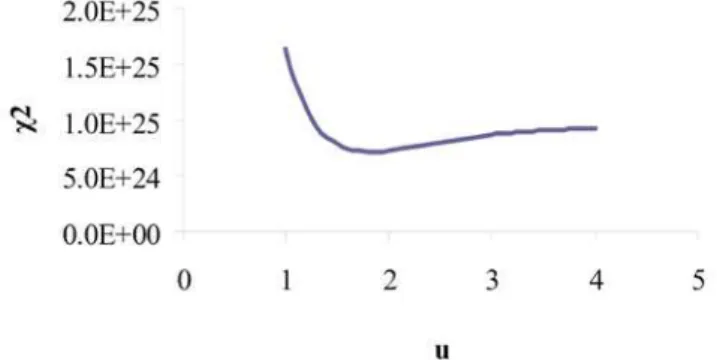
ent over a small interval between data points. Lower exponents produce a surface relatively flat with short blips. An exponent of not only gives seemingly satisfactory results for the general sur-face mapping and description purposes, but also presents the simplest form of calculation as Shepard [9] recommended. Figure 2 proves that leads to the best concurrence with the exact simula-tion. In Cartesian coordinates the distance between two points can be expressed as (3).
Figure 2 Influence of on Chi-Square test function
(3)
Since Shepard's radius function, does not fit multidimensional problems, it is modified as (4) and the rest of the equations remain unchanged.
(4)
where = number of decision variables; = total number of data points; = the number of data points included in the circle with radius (Shepard recommended ); and and = maximum and minimum value of decision variable respectively. To achieve a higher compatibility with the exact simulation, Shepard has introduced several improvements to the original function (i.e. considering directions, determining the slope, etc.). These extra modifications not only increase the computational load, but also are not easily applicable to the multidimensional space hence they are not considered in this research.
4 HARMONY SEARCH ALGORITHM
Harmony Search (HS) algorithm is a replication of a musical performance process. A musician's search to find a better state of musical harmony (a perfect state) [3] is similar to optimization process that seeks to find a global solution (a perfect state) as determined by an objective function. The pitch of each musical instrument determines the aesthetic quality; similarly, the set of values assigned to each deci-sion variable determines the value of the objective function. The optimization procedure of HS algo-rithm consists of the following steps:
2
u =
2
u =
u
n N C
r C = 7 xkmax
min k
X
k
1. Initializing the optimization problem and algorithm parameters: The general form of optimization problem is specified as follows:
(5)
where = an objective function; = optimization variable; and = the set of possible range of each decision variable. The parameters of HS algorithm, that is, HMS, HMCR, and PAR are also specified at this step. HM is a memory space where all the solution vectors (sets of decision variables) are stored which is similar to the genetic pool in GA. This will be shared with IDW as its initial points.
2. Initializing HM: HM matrix shown in (6) is filled with as many solution vectors as the value of HMS. These solutions are randomly generated and sorted according to the values of the objective function,
.
(6)
3. Improvise a new harmony from HM: Memory considerations and pitch adjustments determine if the new harmony vector should be generated from HM. That is, (the value of vari-able for the new vector) is chosen from the values in HM or .The value of HMCR which varies be-tween 0 and 1 will determine where to choose the possible new value as indicated by (7).
(7)
Every component of the new harmony vector, is examined to determine whether it should be pitch-adjusted. This procedure uses the PAR parameter that sets the rate of adjustment for the pitch chosen from the HM as shown in (8).
(8)
The HMCR and PAR parameters, introduced in Harmony Search, help the algorithm find globally and locally improved solutions, correspondingly.
4. Update the HM: The new harmony vector replaces the worst harmony if a better objective function value is obtained. HM is then resorted.
5. Check if the termination criterion is satisfied: When the termination criterion is not satisfied steps 3 and 4 are repeated.
For further information about the HS algorithm see Refs [3, 17-21].
5 THE NEW MULTILEVEL OPTIMIZATION ALGORITHM ( )
f x xi Xi
( )
f x
th i
i
X
In this study, a combination of IDW and HS is employed to decrease the computational effort and improve the convergence rate. The presented method has been applied to a number of truss design problems, which are presented in the next section.
An optimal truss design is one in which the optimal cross-sectional area assigned to each member satisfies the given constraints. Design constraints typically consist of the maximum allowable com-pressive and/or tensile stress in any member of the truss and the maximum allowable deflection of any node [1]. The truss optimization objective function can be expressed as (9).
(9)
where = weight of the truss; = number of members making up the truss; = material density of member ; = length of member ; and = cross-sectional area of member i, chosen from a set of areas between and , where = lower bound and = upper bound. The parameters and represent the stress and deflection of the member of the truss respectively.
The algorithm consists of the following steps:
1. Generating the sample points and initializing HM: sample points are generated by selecting cross-sections from an eligible set of cross-cross-sections. At least one cross-section should be chosen near the up-per bound and one near the lower bound (e.g. and respectively). The remaining selections should be distributed uniformly between these bounds. Then a sample grid matrix ( ) is gener-ated from the chosen cross-sections, where is the number of truss members and should be great-er than or equal to 2 (the minimum numbgreat-er of sample point entries). In othgreat-er words, the entries of sample grid matrix are chosen from those sample points. For instance, (10) shows the formation of SG matrix for 25-bar truss from the sample points 0.5 and 3.0.
(10)
HMS determines the number of cross-sections from SG matrix that HM should be filled with. An exact simulation is applied to each point in HM. Both IDW and HS get their initial points from the same HM.
Note: In (9) the cross-sectional constraint is zero cost, while and impose computational efforts. In the case where and are not satisfied, HM would not be updated. In this case, the algorithm
W m gi
i Li i Ai
l
A Au l u
th i
0.9Au 1.1Al
m
q
recovers the unacceptable solution and by applying superposition principle, makes it more acceptable. That is, the cross-sectional area of each member is multiplied by (11) and then it would be added to HM. Applying such a factor to the cross-sectional area makes the stress and deflection ratios to be as close as possible to 1. The above operation will satisfy the first two constraints mentioned in (9) for all solution vectors, but the cross-sectional constraint may be violated. As HM is filled by order of priority from the lightest to the heaviest truss, which generally implies that HM will be filled from the smallest to the largest cross-sections, the repeated application of algorithm through its convergence process will force the satisfaction of cross-sectional area constraint. For a detailed explanation of the normalization process, assume the algorithm found the solution [0.236, 0.409, 2.094, 1.992, 0.426, 0.459, 1.106, 2.026] which is not acceptable according to the stress and deflection ratios (1.5 and 0.216 respective-ly). However, the solution could be recovered through the normalization process by multiplying the solution to the normalization factor, 1.5, which is obtained using (11). The recovered solution would be [0.354, 0.614, 3.141, 2.988, 0.639, 0.688, 1.658, 3.039], with stress and deflection ratios of 1.000 and 0.144, which satisfies the criteria and could be added to HM. It should also be noted that the only pa-rameter, which affects the performance of the algorithm, is the initial sample points.
(11)
2. Generating a new solution vector: A new solution vector is generated according to (12) where the cross-sectional area of the member is determined using HMCR and PAR (see (7) and (8) respectively).
(12)
where = new cross-sectional area of member; = total number of iterations; and = cur-rent step.
3. Estimating the approximate response: IDW is used to estimate the new solution response. If the new approximate response is better than the worst one stored in HM, the algorithm will proceed to the next step. Otherwise, it will return to the previous step.
4. Evaluating the exact response: An exact response evaluation process is applied to the new generated solution. If the accurate response is acceptable, the worst solution in HM is replaced. Otherwise, the algorithm will return to step 3. In further iterations, as the responses in HM get closer to the optimal response, the distance between the approximate and accurate responses is reduced. Numerical exam-ples show that the most of unnecessary and expensive calculations are eliminated in the early iterations where the responses are far enough from the optimal response.
5. Checking the termination criteria: The algorithm terminates in a certain number of iterations ( i.e. ). Although the most of the meta-heuristic algorithms have some other criteria together with maximum iterations, we avoided to adopt such criteria here, because the IDW reduces the number of HS (exact analysis) iterations. On the other hand, the criteria excluding maximum
itera-new i
A ith K I
K = I
tions may lead to a premature solution. If the termination criterion is not met, the algorithm repeats steps 3 and 4.
6. Polishing the result: A semi-tabu algorithm is applied to the final solution to obtain a better solution. The semi-tabu is to find a smaller cross section area for each member to reach a better solution, while satisfying the criteria. This is achieved by reducing each area by multiplying by 0.95 in a loop, while satisfying the criteria. It should be noted that only one member is reduced in each loop.
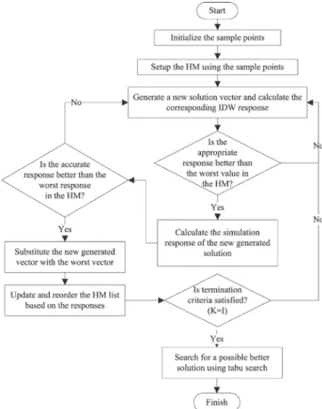
Figure 3 shows the optimization procedure of the IDW+HS algorithm.
Figure 3 Optimization procedure of IDW+HS algorithm
6 COMPUTATIONAL EXPERIMENTS
The efficiency of the algorithm was evaluated through some numerical examples. To investigate the computational cost and convergence rate, three examples (10, 25, and 72-bar truss) are selected from refs [1-4]. The algorithm was developed using Python programming language and ran on a Centrino, 1.4 GHZ computer. The structural analysis also was done using OpenSees code.
The 10-bar truss is discussed in detail to show the efficacy of the algorithm, and the other examples are given for further investigations. These problems have been widely used as benchmarks to test and veri-fy the efficiency of many different engineering optimization methods.
6.1 Ten-bar truss
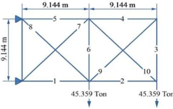
Figure 4 shows the geometry and support conditions for two-dimensional cantilever 10-bar truss with a single loading condition.
Figure 4 Configuration of 10-bar truss
The material used in this structure has a modulus of elasticity of and a mass
densi-ty of . The design constraints are: maximum allowable stress in any member of the
truss ; maximum deflection of any node (in both vertical and horizontal direc-tions) . The upper and lower limits of cross-section areas of each truss member
. The sample points by which the sample grid is generated are 1.0 and 30.0. Figure 5 compares the convergence rate of the proposed algorithm with that of some other algo-rithms (GA, ACO, HS, IDW+HS, etc.). The IDW+HS has been already compared with the other pure me-ta-heuristic algorithms by the authors [16]. Here the IDW+HS is compared with the new modified algo-rithm. The comparison indicates that although the IDW+HS+Tabu fits the IDW+HS at the early stages, in the final steps, the semi-tabu algorithm leads to a lighter design. The exact design weight is shown in Table 1. It can be seen that the new algorithm designed a lighter structure compared to the IDW+HS algorithm (4893 vs 4963), in a fewer iterations (682 vs 1870).
Figure 5 The convergence diagram for minimum weight design of 10-bar truss with various algorithms Table 1 The best solutions obtained from various algorithms for 10-bar truss
Truss member ACO GA: Camp et al. Mahfouz GA HS IDW+HS IDW+HS+Tabu 1 29.90 28.92 33.50 30.05 29.85 29.88 2 0.10 0.10 1.62 0.27 0.53 0.14
68.948
E = GPa
3 26.10 24.07 22.90 22.86 22.81 20.53 4 15.40 13.96 14.20 14.58 14.54 13.84 5 0.10 0.10 1.62 0.10 0.10 0.37 6 0.50 0.56 1.62 0.28 0.73 1.02 7 20.90 21.95 22.90 20.64 20.58 18.18 8 7.40 7.69 7.97 8.11 7.31 7.04 9 0.10 0.10 1.62 0.24 0.10 1.06 10 18.70 22.09 22.00 20.69 21.01 23.33 Weight (lb) 4994 5076 5491 4982 4963 4893
Iterations 12000 15000 8000 5000 1870 682
6.2 Twenty Five-bar Truss
Material properties and design constraints:
; ; ; ;
; sample points = 0.5 and 3.0.
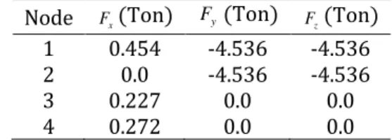
Table 2 Single load case for 25-bar truss
Node (Ton) (Ton) (Ton) 1 0.454 -4.536 -4.536 2 0.0 -4.536 -4.536 3 0.227 0.0 0.0 4 0.272 0.0 0.0
Table 3 Multiple load case for 25-bar truss
Case Node (Ton) (Ton) (Ton)
1
1 0.454 -4.536 -2.268 2 0.0 -4.536 -2.268 3 0.227 0.0 0.0 6 0.227 0.0 0.0 2 1 0.0 9.072 -2.268
2 0.0 -9.072 -2.268
x
F Fy Fz
x
F Fy Fz
Figure 6 Configuration of 25-bar truss
Figure 7 The convergence diagram for minimum weight design of 25-bar truss under single load case with various algorithms
Table 4 The best solutions obtained from various algorithms for 25-bar truss under single load case
Group Truss member ACO GA: Camp et al. HS IDW+HS IDW+HS+Tabu 1 1 0.10 0.10 0.12 0.28 0.52 2 2-5 0.30 0.50 0.17 0.30 0.40 3 6-9 3.40 3.40 3.40 3.40 3.04 4 10-11 0.10 0.10 0.12 0.11 0.56 5 12-13 2.10 1.90 1.23 1.73 1.64 6 14-17 1.00 0.90 0.82 0.91 0.64 7 18-21 0.50 0.50 0.94 0.53 0.51 8 22-15 3.40 3.40 3.35 3.39 3.37 Wight (lb) 485 485 482 476 451 Iterations 7700 15000 5000 2838 166
Figure 8 The convergence diagram for minimum weight design of 25-bar truss under multiple load case with various algorithms
Table 5 The best solutions obtained from various algorithms for 25-bar truss under multiple load case
Group Truss member ACO GA: Camp et al. HS IDW+HS IDW+HS+Tabu 1 1 0.01 0.01 0.10 0.10 0.41 2 2-5 2.00 2.01 1.65 2.05 2.21 3 6-9 2.97 2.95 3.12 2.97 2.55 4 10-11 0.01 0.01 0.13 0.19 0.32 5 12-13 0.01 0.03 0.11 0.12 0.43 6 14-17 0.69 0.68 0.53 0.67 0.63 7 18-21 1.68 1.68 2.04 1.57 1.38 8 22-15 2.67 2.68 2.80 2.64 2.49 Wight (lb) 545.53 545.80 559.45 542.14 516.82
Iterations 7700 15000 5000 2838 557
6.3 Seventy Two-Bar Truss
Material properties and design constraints:
68.948
E = GPa; 2.768T 3
m
g = ; ; ;
; sample points= 0.05 and 2.20
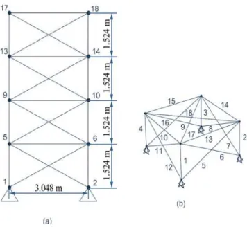
Figure 9 Configurations of 72-bar truss Table 6 Nodal coordinates of story for 72-bar truss
Node X (m) Y (m) Z (m) i+1 -1.524 -1.524 1.524i i+2 1.524 -1.524 1.524i i+3 1.524 1.524 1.524i i+4 -1.524 1.524 1.524i
Table 7 load conditions for 72-bar truss
Case Node (Ton) (Ton) (Ton)
1
17 0.0 0.0 -2.268 18 0.0 0.0 -2.268 19 0.0 0.0 -2.268 20 0.0 0.0 -2.268 2 17 2.268 2.268 -2.268
th i
x
F Fy Fz
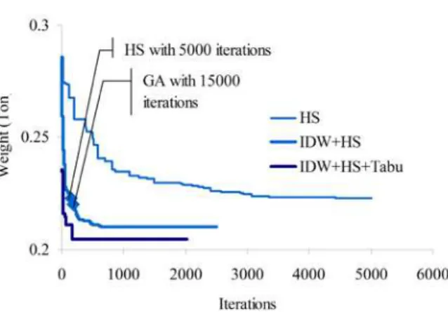
Figure 10 The convergence diagram for minimum weight design of 72-bar truss with various algorithms
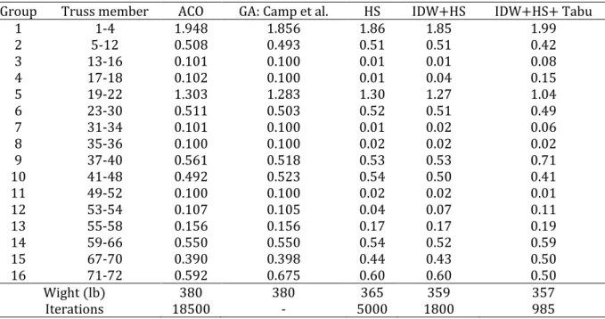
Table 8 The best solutions obtained from various algorithms for 72-bar truss
Group Truss member ACO GA: Camp et al. HS IDW+HS IDW+HS+ Tabu 1 1-4 1.948 1.856 1.86 1.85 1.99 2 5-12 0.508 0.493 0.51 0.51 0.42 3 13-16 0.101 0.100 0.01 0.01 0.08 4 17-18 0.102 0.100 0.01 0.04 0.15 5 19-22 1.303 1.283 1.30 1.27 1.04 6 23-30 0.511 0.503 0.52 0.51 0.49 7 31-34 0.101 0.100 0.01 0.02 0.06 8 35-36 0.100 0.100 0.02 0.02 0.02 9 37-40 0.561 0.518 0.53 0.53 0.71 10 41-48 0.492 0.523 0.54 0.50 0.41 11 49-52 0.100 0.100 0.02 0.02 0.01 12 53-54 0.107 0.105 0.04 0.07 0.11 13 55-58 0.156 0.156 0.17 0.17 0.19 14 59-66 0.550 0.550 0.54 0.52 0.59 15 67-70 0.390 0.398 0.44 0.43 0.50 16 71-72 0.592 0.675 0.60 0.60 0.50 Wight (lb) 380 380 365 359 357 Iterations 18500 - 5000 1800 985
7. CONCLUSION
This paper describes a surrogate-based optimization algorithm. It is a combination of a metamodel and a meta-heuristic algorithm. Most of the meta-heuristic algorithms (e.g. GA, HS, and ACO) employ a large initial population size, which leads to a large and costly number of function evaluation and suffer from slow convergence. These prohibitive factors are more pronounced when applied to exact simulation. IDW+HS+Tabu algorithm implements the optimization process in two steps. First, the IDW is applied to eliminate the unnecessary calculations. Then the remaining solutions are processed for exact simulation. Then superposition principle is applied to normalize the result of exact simula-tion. Finally HM is updated by the results. The algorithm was applied to four truss design problems. The obtained results showed that the proposed method not only reduces the computational effort
but also significantly improves convergence rate. As shown above, the proposed algorithm saves the computational cost from 86 to 99 percent.
References
1. Camp, C.V.,Bichon, B.J.: Design of Space Trusses Using Ant Colony Optimization. J. Struct. Eng. ASCE. 130, 741-751 (2004)
2. Kaveh, A., Gholipour, Y.,Rahami, H.: Optimal design of transmission towers using genetic algorithm and neural networks. International Journal of Space Structures. 23(1), 1-19 (2008)
3. Lee, K.S.,Geem, Z.W.: A new structural optimization method based on harmony search algorithm. Comput. Struct. 82, 781-798 (2004)
4. Rahami, H., Kaveh, A.,Gholipour, Y.: Sizing, geometry and topology optimization of trusses via force method and genetic algorithm. Eng. Struct. 30, 2360-2369 (2008)
5. Barthelemy, J.F.M.,Haftka, R.T.: Approximation Concepts for Optimum Structural Design – A Re-view. Struct. Optimization. 5(3), 129-144 (1993)
6. Jin, R., Chen, W.,Simpson, T.W.: Comparative studies of metamodelling techniques under multiple modelling criteria type. Struct. Multidiscip. 23(1), 1-13 (2001)
7. Martin, J.D.,Simpson, T.W.: A Study on the Use of Kriging Models to Approximate Deterministic Computer Models. ASME Conference Proceedings. 2003(37009), 567-576 (2003)
8. Jurecka, F.: Robust design optimization based on metamodeling techniques. Shaker Verlag GmbH, Germany (2007)
9. Shepard, D.: A two-dimensional interpolation function for irregularly-spaced data. Proceedings of the 1968 23rd ACM national conference (1968)
10. Bonte, M.H.A., Boogaard, A.H.,Huetink, J.: Solving optimization problems in metal forming using Finite Element simulation and metamodelling techniques. Apomat conference (2005)
11. Hu, W., Li, E., Li, G.Y.,Zhong, Z.H.: Development of metamodeling based optimization system for high nonlinear engineering problems. Advances in Engineering Software. 39, 629-645 (2008) 12. Kleijnen, J.: Kriging metamodeling in simulation A review. Eur. J. Oper. Res. 192, 707-716 (2009) 13. Lee, T.H.,Jung, J.J.: A sampling technique enhancing accuracy and efficiency of metamodel-based
RBDO: Constraint boundary sampling. Comput. Struct. 86, 1463-1476 (2008)
14. Sakata, S., Ashida, F.,Zako, M.: Structural optimization using Kriging approximation. Comput. Met-hod. Appl. M. 192, 923-939 (2003)
15. Friedman, J.H.: Multivariate adaptive regression splines. Ann. Statist. 19(1), 1-67 (1991)
16. Yaghoub Gholipour, M.M.S.: Decreasing Computational effort using a new multi-fidelity metamode-ling optimization algorithm. Lisbon, Portugal. (2010)
17. Geem, Z.: State-of-the-Art in the Structure of Harmony Search Algorithm. Springer Berlin / Heidel-berg. 1-10 (2010)
18. Geem, Z.W.: Novel derivative of harmony search algorithm for discrete design variables. Appl. Math. Comput. 199, 223-230 (2008)
19. Geem, Z.W.: Music-Inspired Harmony Search Algorithm: Theory and Applications. Springer Publis-hing Company, Incorporated (2009)
20. Lee, K.S.,Geem, Z.W.: A new meta-heuristic algorithm for continuous engineering optimization: harmony search theory and practice. Comput. Method. Appl. M. 194, 3902-3933 (2005)
21. Mahdavi, M., Fesanghary, M.,Damangir, E.: An improved harmony search algorithm for solving optimization problems. Appl. Math. Comput. 188, 1567-1579 (2007)
22. Brus, D.J., De Gruijter, J.J., Marsman, B.A., Visschers, R., Bregt, A.K., Breeuwsma, A.,Bouma, J.: The performance of spatial interpolation methods and choropleth maps to estimate properties at points: A soil survey case study. Environmetrics. 7(1), 1-16 (1996)
23. Webster, R.,Oliver, M.A.: Sample adequately to estimate variograms of soil properties. Journal of Soil Science. 43(1), 177-192 (1992)
24. Gallichand, J.,Marcotte, D.: Mapping clay content for subsurface drainage in the Nile Delta. Geo-derma. 58(3–4), 165-179 (1993)
25. Anthony, A.G., Jane, M.D., Robert, N., Bernard, G., Raphael, T.H., William, H.M.,Layne, T.W.: Noisy Aerodynamic Response And Smooth Approximations In HSCTDesign.
26. Barton, R.R.: Metamodels for simulation input-output relations. ACM: Arlington, Virginia, United States. 289-299 (1992)
27. Shao, W., Deng, H., Ma, Y.,Wei, Z.: Extended Gaussian Kriging for computer experiments in engi-neering design. Engiengi-neering with Computers. 28(2), 161-178 (2012)