Private equity : what happens next?

(1)

Private Equity: What

Happens Next?

Miguel Machete Botelho

Dissertation written under the supervision of Professor

Pramuan Bunkanwanicha

Dissertation submitted in partial fulfilment of requirements for the

International MSc in Management, at Universidade Católica Portuguesa

(2)

(3)

Private Equity: What Happens Next?

Miguel Machete Botelho

Abstract:

Previous academic research has focused on Private Equity funds’ superior performance, when compared to respective benchmarks. However, there is still a question to be answered: what happens after these funds’ targets leave Private Equity’s protective wing? From a sample of 426 observations, from which 180 had previously been funded by Private Equity, in both US stock exchanges, we built a first-differences regression model to investigate the subject. We found evidence showing that Private Equity’s superiority during funds’ lifetime is paid away in the years after. Our sample revealed a negative effect detected on long-term performance of firms whose Initial Public Offerings were Private Equity-backed. The data collected suggests a possible variation of the negative impact, depending on the industrial sector. There is also evidence that smaller firms are more affected than larger firms, by the identified Private Equity effect. The percentage of outstanding shares issued at IPO is positively correlated with the negative impact under scrutiny, when less than half of the total equity had been issued. Nevertheless, one must be cautious when interpreting the results, as our performance measures are scaled by the market capitalization, which is subject to investors’ overvaluation.

(4)

(5)

Private Equity: O Que Se Segue?

Miguel Machete Botelho

Sumário:

A literatura académica tem vindo a concentrar-se na rentabilidade superior dos fundos de Private Equity, quando comparados com os respectivos benchmarks. No entanto, uma questão permanece por responder: o que acontece às empresas previamente detidas por estes fundos depois de deixarem de o ser? De uma amostra de 426 observações, das quais 180 foram previamente financiadas por Private Equity, em ambas as bolsas de valores dos EUA, construímos um modelo de regressão de primeiras diferenças para investigar o assunto. Encontrámos provas de que a rentabilidade superior verificada em Private Equity, durante a vida dos fundos, tem um reverso nos anos seguintes. A nossa amostra revelou um efeito negativo detectado no desempenho de longo prazo das empresas submetidas a Ofertas Públicas de Aquisição por fundos de Private Equity. Os dados recolhidos sugerem uma possível variação desse efeito, dependendo do sector industrial a que cada empresa pertence. Há também evidências de que empresas de menor dimensão de activos são mais as afectadas pelo efeito negativo de Private Equity. A percentagem de ações em circulação emitida em OPA está positivamente correlacionada com o efeito negativo identificado, o que, consequentemente, nos levou a resultados, estatisticamente verificados, de que este se encontra presente apenas perante percentagens inferiores a cinquenta porcento. Contudo, é preciso ter em conta que, na interpretação destes resultados, as medidas de desempenho utilizadas foram ajustadas pela capitalização de mercado, sujeita à sobrevalorização por parte dos investidores.

(6)

Acknowledgements:

Writing this Master Thesis was a journey full of ups and downs. I recognise it would not be accomplished without the unconditional support of my family, friends, and professors, all of whom gave a special contribution, that allowed me to add value to this project.

To my parents, who gave me the opportunity of studying in two great universities, who opened the doors and helped me going through them. I am very grateful to my father, who gave me new ideas and ways to approach the subjects. To my mother, for all those hours spent reviewing for mistakes and inventing new approaches, even when those sessions were depriving long hours of sleep. I value both as well for the efforts made to put me in contact with the right people, that could offer me a hand when the path was getting hard to cross.

To my siblings, Gonçalo and Marta, and to Sofia, who showed me new ways to face the hurdles along this path. I must recognise that sometimes I could not dedicate the right amount of time and good mood to spend with you, so I apologize for when this thesis was put first before our relationship.

To my grandparents, Mimi, Rui and Bé, whose encouragement and advice were always welcomed. To my grandfather, Nuno, who will carry on inspiring me in all my challenges. To Professor Gonçalo Rocha, who provided me with the right help, at the right time.

Finally, I would like to give a special thanks to my thesis’ supervisor, Professor Pramuan Bunkanwanicha, who accepted to support me through this journey.

(7)

List of Tables:

Table 1: Variables’ description ... 10

Table 2: Coefficients’ description ... 15

Table 3: Descriptive Statistics ... 16

Table 4: Model overview ... 17

Table 5: Regression models by the class of firm size ... 23

Table 6: Regression models by issue date of IPO ... 24

Table 7: Regression models by the class of firm size ... 27

List of Figures:

Figure 1: Total number of IPOs per year ... 10

Figure 2: Total market capitalization by year of IPO ... 10

Figure 3: Representation of each sector in the sample ... 11

Figure 4: Boxplot representing the distributions in both dependent variables’ differences ... 15

Figure 5: Comparison between the values obtained in regression and real values (ROE) ... 18

Figure 6: Comparison between the values obtained in regression and real values(ROA) ... 18

Figure 7: Difference in ROE across sectors ... 20

Figure 8: Difference in ROE by the leverage ratio ... 21

Figure 9: Difference in ROE by assets’ size ... 22

Figure 10: Difference in ROE by age at IPO ... 25

(9)

1. Introduction:

Private Equity (PE) funds invest in firms in need of capital to either recover from financial difficulties or to fuel growth. They acquire these targets with the purpose of selling them, on average, four to seven years later. During this period the funds’ managers often play the role of activist shareholders, in order to fulfil their agenda within the intended timeline.

Previous academic research has found that the way PE manages its investments in companies throughout the funds' lifetime, has led to an-above average performance when benchmarked against companies that didn’t receive PE investments. But this leads us to one of the basics in economics: there are no free lunches. Or are there? What happens to these firms after leaving the funds' protective wing? There are many different opinions regarding the subject. Critics argue that excessive levels of debt contracted and a focus on quick returns, during funds' lifetime, destroy value in the long run. Supporters defend that specialized financing agents, enable value growth without damaging future performance. Who is right? Do PE fund managers compromise the future long-term performance of their investments to maximize their exit price, or is it indeed, a free lunch?

This study intends to fill in the gap identified in academic research, by investigating the impact in the post-exit value of a company, caused by PE management techniques. We are going to compare the value of companies immediately after leaving the portfolio of PE funds with that of three years later, in order to study whether performance is, in fact, different between PE-backed and non-PE-PE-backed IPOs.

The performance of Initial Public Offerings (IPOs), as an exit strategy, will be the event taken under scrutiny. We will approach performance analysis through this path as it leads to comparing the strategy implemented by PE funds’ targets with the one applied by other firms in the same situation. An IPO is the third most common exit strategy applied by PE funds (Kaplan & Strömberg, 2009). Adding this idea to the fact that the new owners of the exited companies are the same for every observation (the market), we decided to study performance on firms going under the same conditions, hence the same exit strategy: the IPO.

When comparing all the IPOs issued worldwide, the United States is by far the most prolific market in terms of the number of deals that happen every year (PwC). We identified it as an opportunity for our investigation, since it provided a large number of observations, and therefore a better understanding of the what occurs, in the long-term, when firms are PE-backed.

(10)

From a sample of 426 observations, 180 of which were PE-backed, taken from the 2 largest stock exchanges in the United States – NYSE and NASDAQ – we analysed what differed between treatment (PE-backed) and control (non-PE-backed) groups, in terms of their long-term performance, defined by the three years following the date of admission to the stock exchange. These observations were collected, considering all the firms listed in these two markets, from the year 2010 to 2014. Two samples were collected for each observation, one at the end of the IPO year and a second instance three years later.

The test where this thesis is centred focuses on the null hypothesis: “Private Equity’s influence on targets still remains after the exit strategy”. The alternative hypothesis to our investigation is “Private Equity’s impact after the exit strategy can be neglected”.

Our main finding was a long-term, negative, impact on return on equity, created on companies previously financed through PE. Later, we dived deeper into this effect and identified where this financing mechanism had its strongest influence. In fact, the intrinsic characteristics of observed companies, such as the business sector in which they operate, their size, and proportion of shares admitted for listing in an IPO, in relation to the amounts of shares outstanding, all affect our initial conclusions.

The remainder of our study is organized as follows: In Section 2 we describe the status quo in academic literature, explaining why PE-backed firms perform better during the funds’ lifetime. This section bridges with current knowledge to a focus on what is documented about the consequences for the long-term performance of companies. In Section 3, we present the steps we took to construct our dataset and explain how we designed the regression model to study operating performance in the long-run. Section 4 details the results obtained during this research and provides a possible explanation for the outputs of the model, whilst laying out any potential limitation of the model. In Section 5, we conclude the investigation.

(11)

2. Literature Review:

Ever since its conception, in the 1980s, there has not been a homogeneous opinion about PE (Kaplan & Strömberg, 2009). Supporters defend it creates economic value on its targets and improves their operations’ efficiency. Critics state PE takes advantage of market timings and provide their targets with incentives on short-term performance, through reductions in capital expenditures and staff, harming the prospects for long-term projects.

PE’s two major types are VC and Leveraged Buyout (LBO) funds (Metrick & Yasuda, 2010). The first kind consists mainly of targeting minority ownership positions in young firms in need of capital to expand their operations, helping them growing their activities and entering new markets. LBO’s targets are usually majority control of more mature and undervalued firms. The strategy for both cases is to buy at low cost and sell the targets, four to seven years later, on average, a much higher value than the initial deal.

For many years, researchers have studied performance on PE funds. Harris et al. (2014) found out that these funds generally beat the market index (S&P 500) from the 1980s to 2000s, an outperformance of at least 3% a year.

Diving deeper into this theme, it has been studied the factors that help us understanding it. When analysing PE funds, authors focused on the people behind them. Studying whether the performance was depending on the funds’ management led some authors to a different conclusion from investors’ usual expectation. The studies revealed that different funds have different performances, not being significantly influenced by their managing partners, in the post-2000s PE funds (Harris, Jenkinson, Kaplan, & Stucke, 2014). Brown et al. (2017) confronted these conclusions, when they acknowledged performance consistencies from one fund to another, hypothesising decreases in performance as being either due to loss of talent (managers leaving for other firms) or increased market competition.

Even though the findings by Harris et al. (2014), referred above, are surprising, Kaplan & Schoar (2003) identified evidence, stating that successful fund managers tend to carry on their activities by creating larger funds. According to Metrick & Yasuda (2010), LBO is regarded as more scalable than VC, since it uses more capital to invest in larger firms, relying on the idea that what they apply to smaller investments may succeed in larger ones. For VC, as these funds invest in much smaller firms, more money leads to investing in more firms, which may lead to the underperformance explained by, losing focus on each investment.

(12)

We find challenging the fact of larger PE funds being able to perform better. These events go against what has been observed by Moeller et al. (2004; Cao & Lerner, 2009), who found out that larger firms tend to perform more poorly in mergers and acquisitions when compared to smaller firms. The authors concluded that acquisitions made by large firms tend to result in large dollar losses, whereas the ones made by smaller firms tend to result in small dollar gains. PE funds’ main source of income is capital gains, which leads us to question what these funds do to obtain such results.

As mentioned earlier, PE funds focus their investment strategies on buying to sell, after firms’ structural interventions. The usual time horizon of investments lies between four and seven years. After this period, an exit strategy is put in motion, by selling the invested firm, making returns on capital gains. Kaplan and Strömberg (2009) identified selling to strategic acquirers, selling to a secondary LBO fund and IPOs as the exit strategies most commonly used by PE between 1980 and 2007.

Directing to the reasons why we find the targets of PE funds better performing than the others, Kaplan and Strömberg (2009) define the intervention as changing the structure on three fields: financial, governance and operational.

Regarding the first one, financial restructuring transformations aim mainly to change management’s incentives and leverage. PE-backed firms management are given a large equity upside, biasing the decisions into creating higher enterprise value in the short-term. They also present higher debt-to-equity ratios than the average, which discourages wasting money on unnecessary projects that would hinder the payments of interests and principal.

Concerning the second field, governance, alterations are predominantly on the Board size and meetings periodicity, together with management turnover. When assuming their targets’ ownership, PE funds decrease the size of the Board and increase the number of meetings per year. These measures improve monitoring on the activities and decrease information asymmetry. Moreover, the poorly performing management under their control is replaced, focusing on maximizing the value of the firm.

In the operational field, the changes are achieved through the introduction of industry expertise, hiring professionals and making use of external/internal consulting groups. In this area, PE funds tend to intervene in order to make firms more efficient, thus maximizing their value. According to supporters of PE, these different types of structuring engineering are responsible for the success of the fund’s exceptional performance during their lifetime (Harris, Jenkinson,

(13)

& Kaplan, 2014). Nonetheless, as described before, there is no unanimous opinion on what concerns PE’s strategies. In fact, evidence found by Sincerre, Sampaio, Famá, and Flores (2019), in the Brazilian market, identified that, even the new management of firms previously financed by PE, and non-PE-backed, had different approaches still, after the IPO. The purpose of this thesis is to follow the critics’ viewpoint and to test whether or not their concerns are legitimate.

From the conclusions drawn by Lee and Wahal (2004), we may infer that investors trust more on firms previously financed by PE to perform better in the market. The authors conclude that the more recognised a firm is before going public, the higher the costs from underpricing. According to Chan et al. (2004), stock performance does not depend purely on investors’ expectations, but also on operating performance, as there was found a positive correlation with this second factor. Following this line of thought, we will study if investors’ expectations are aligned with the actual performance of previously PE-owned firms.

(14)

3. Methodology:

In this Section, we will describe the construction of our dataset and how we achieved the regression model used for the analysis

3.1. Data:

Collecting and transforming the data to elaborate on this thesis was not an easy process. It was necessary to go through various steps before achieving the final sample.

3.1.1. Collecting market observations:

When analysing the IPOs worldwide, the United States stood out from other markets by the number of deals made each year. This emerged as an opportunity for this study, as more observations allow a better understanding of the real effects occurring.

The data studied in this dissertation is composed of IPOs taking place between 2010 and 2014 in the New York Stock Exchange (NYSE) and NASDAQ. Assembly was made through the information available in Thompson Reuters Eikon and Wharton Research Data Services. The period of study was selected with the objective of collecting the most recent events, ensuring the firms carried on their public status after the three years of analysis.

To obtain a table with all the required information, for the purpose of this study, the first step was to collect all observations in the defined period, by researching the events available on Thomson Reuters Eikon, counting a total of 1130 firms. Not all the events were adequate for analysis, so several criteria were applied to select the firms suitable for our research.

The first criterion was geographical. Performance may be biased by the country where firms are ensconced, so we narrowed our range to the United States market. As the analysis is focused on American stock exchanges, we intended to use a sample as large as possible, thus focusing on the country involving most firms.

The second measure was related to the type of IPO issued. Some events registered by Thomson Reuters Eikon were funds being issued, which cannot be used for our analysis. We want to study operating performance measures, and funds group various firms, which would create noise in our conclusions. Moreover, many indicators used in our regression are not available for funds and others would create too much noise in our conclusions. Hence, we decided to exclude these from the analysis.

The third test performed was to verify whether or not the firm had stayed in the public stock market for three fiscal years, after the IPO. We intended to construct panel data for long-term

(15)

performance, by observing two distinct periods, the IPO year and three years afterwards. When the firm could not be observed in the stock market three years later, after the IPO, it was removed from the sample.

The fourth gauge applied was to take out of the sample all observations that were intervened by PE funds during the period being studied. Since our study is focusing on the impact of PE after leaving the firms’ ownership, these observations would be biasing our conclusions, therefore were excluded. Our objective was to evaluate whether the culture implemented by PE on their targets still has its influence after the funds’ maturity. Having this in mind, we could not include in our observations cases where the firm was still under PE possession during the period studied. The final filter applied on our dataset was performed by checking if all the information required was available in both databases, Thomson Reuters Eikon and Wharton Research Data Services. When it was not possible to access the information, we decided to remove the observation from the sample.

Once carried out these examinations, the final sample had 426 observations. From these events, 180 were PE-backed IPOs, accounting for a total of 42% of the studied occurrences.

3.1.2. Creating a panel dataset:

A panel dataset construction involves identifying two (or more) observations in time for the same individual. To construct such a sample, one needs to observe different individuals in various moments in time. Our sample was constructed in a way that each firm was observed two times: the first period, t-1, was the IPO end; the second period, t, was the third year-end after the IPO.

Every variable, described in 3.2, has been collected for each moment required to define both extremes of the time-frame under investigation. Later, a new variable, Post, was added to the sample, taking either the value of 0 or 1, depending on whether the observation was collected at the end of the IPO year or three years later.

The final dataset had ten variables, as described in Table 1, and 852 observations, 426 each period.

(16)

Table 1: Variables’ description

The following table defines the different variables that compose our dataset by the symbol applied in regressions. Description contains a brief explanation of what information each variable involves.

Symbol Description

Ticker Unique identifier of each firm

Year Year when IPO was issued

PE Defining whether the firm had contact with PE before the IPO or not

IN2DROE Average ROE of the two-digit SIC code defined industry level IN2DROA Average ROA of the two-digit SIC code defined industry level LA Logarithmic function of assets market value proxy

DE The Leverage ratio, debt to equity, in market values

Post Defining whether the observation was collected at the end of the IPO year or three years later

ROE Ratio defined by net income divided by equity market value at the end of the fiscal year

ROA Ratio defined by operating income divided by assets market value at the end of the fiscal year Figure 1: Total number of IPOs per year

The figure below presents the total number of deals collected in our sample, differentiating PE’s targets and other firms. In the x labels, we may find the five years under investigation. In the y labels, we find the number of deals occurred.

Figure 2: Total market capitalization by year of IPO

The figure below presents the total amount collected when issued the IPO, differentiating PE’s targets and other firms. In the x labels, we may find the five years under investigation. In the y labels, we find the sum of money raised through all the IPOs issued, in millions of USD.

0 20 40 60 80 100 120 140 2010 2011 2012 2013 2014

Number of IPOs Issued By Year

PE Other $ 020 $ 040 $ 060 $ 080 $ 100 $ 120 $ 140 $ 160 2010 2011 2012 2013 2014 M il li on s Market Capitalisation PE Other

(17)

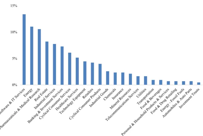
Figure 3: Representation of each sector in the sample

The figure below presents the weight each industrial sector has within our sample. In the x labels, we may find the sector name. In the y labels, we find the percentage of our whole sample, in terms of IPOs, represented by each sector.

3.2. Study variable and performance measures:

During this investigation, we used a dummy variable to analyse the effect of PE on performance. PE was constructed through observing the historical relationship of each individual observation with PE Funds, using Thomson Reuters Eikon. The dummy variable allows us to make the distinction between treatment and control groups. The latter consists of all observations non-PE-backed. The former are the firms affected by PE, that may still be influenced by these funds even after their leaving.

If, before the IPO date, the observation had been in possession of a fund, the variable would take the value 1, otherwise it would take the value 0. There are some limitations regarding this method, as it does not differentiate the various types of exiting PE, which could lead to different results. We will study the PE’s effect as a whole, disregarding the types of funds that backed the issuance.

Afterwards, we made an interaction with the variable Post. The result, PE_Post, was a variable

0% 5% 10% 15%

(18)

To understand the effect of PE funds in the long-term performance of the firms they invest in, we decided to analyse Returns on Equity (ROE) and Returns on Assets (ROA).

As a matter of fact, ROE is commonly known as a measure of management’s effectiveness in the company’s usage of assets to create profits. It will be the first dependent variable. PE influences management’s culture and the operational performance of firms, which leads to heterogeneous opinions on whether it is beneficial or not (Kaplan & Strömberg, 2009). Through the observation of the PE on this variable we intend to provide with some insights that may help investors making their own opinion regarding this subject. ROE is calculated through the Net Income at the end of the fiscal period divided by the market capitalization within the same time range.

ROA is a good proxy to measuring firms’ efficiency of assets, thus it was used as our second

dependent variable. This measure scales the management competence in order to use the assets efficiently. It weights PE influence on making the most of the productive assets in the long-term. ROA, however, has its limitations, namely scaling an operating variable (operating income) by another value, involving also non-operating assets (Barber & Lyon, 1996). In order to make this indicator as useful as possible for interpretation, the value of assets used has been submitted to two different corrections. The first approximation was intended to achieve the market value of assets. As our sample only included observable book values, we decided to correct these, by adding the book value of shareholders’ equity and deducting its market capitalization. The second step was to remove one item, common to every observation, that does not create added value, concerning the firms’ operations: cash. By the end of these two correction stages, we achieved an approximation of cash-adjusted assets’ market value. Later, we divided the operating income by this amount, reaching our second dependent variable for this thesis: ROA. Even though we made these values more suitable for analysis, we still need to be cautious to their limitations, like being constantly undervaluing the efficiency of the assets, as we are keeping in our denominator some non-operating assets (Barber & Lyon, 1996). In spite of this situation, we can be confident in our comparative analysis, as the whole sample is submitted to the same approximations, thus our results are going to be comparable across different observations.

3.3. Control Variables:

The control variables to be applied are effects that may vary during the period under investigation. Hence, the average returns of the industry (ROE or ROA), a proxy of the market

(19)

value of assets, the leverage ratio and the year when the IPO occurred helped us understanding better the effect of PE during the three years that follow the entrance in the stock market. According to Barber and Lyon (1996), samples must be controlled for different industries. This process was achieved by computing the industry two-digit SIC average value of the different dependent variables, in market values, at the end of IPO year and three years after. The market average was extracted from Wharton Research Data Services. The variables allowed us to control for industry abnormal performance, during the period of study of each observation. To mark changes on company’s value within the time-frame under scrutiny, we opted to include in our model a variable that marked abnormal growth of assets throughout different observations. The variable used in this situation was a proxy of the market value of assets, similar to the denominator of our dependent variable ROA, but including also the amount of cash, as we believe changes in the whole size of the firms must be accounted for. Later, a logarithmic transformation was applied to the component in order to obtain a distribution close to the normal density function, resulting in the variable LA.

Leverage influences both, the management culture and the earnings of firms. In fact, having higher values of debt, results into more disciplined management of the firm's resources. This component also has an influence on net income through interest tax shields. One other consequence of changes in leverage is the risk of financial distress. In fact, the higher values for the ratio result in the business being perceived as more risky, by the investors. The variable DE was created by dividing the net assets (a proxy of the market value of assets subtracted the market value of equity) by the market value of equity.

The last characteristic we wanted to control for was the timing of the IPO. As the market is not constant, occurring growth and recession economic cycles, we must consider these effects in our model. Following this line of thought, we created a cluster variable, Year, that marks the point in time when the data was extracted (both the IPO year and the period Post IPO, three years later).

Some of the variables described present outliers, which would bias our conclusions on modelling on the mean. To correct these observations, we applied the same procedure as used by Barber and Lyon (1996), winsorizing all information at the first and 99th_{percentiles. The}

values outside these limits took the same values as the percentiles, in order to avoid excluding observations.

(20)

3.4. First differences:

Throughout the period under analysis, some characteristics specific to each firm are not observed, such as life-cycle and the amount offered at IPO. Although this hurdle is present in our data, it can be mitigated through the use of panel data. The model applied in this thesis includes two periods, the year when the IPO was issued and three years later, computing the influence of treatment (having been PE-backed) throughout this range.

Academia has investigated several methodologies to evaluate the behaviour of the treated population during events. From the various regressions used in the past, those that provided more accurate results were the ones comparing one period to the state the observation found itself in a period before. Panel data analysis is set to evaluate the difference between the changes in the value under scrutiny, between the period of the event, t, and the one prior to it, t-1, or Δ𝑦 = 𝑦_𝑡− 𝑦_𝑡−1. Dependent variables’ distributions are graphically represented in Figure 4. Moreover, comparing differences between the performance of treated and control groups results in more powerful statistics, as Barber and Lyon (1996) found evidence upholding this conclusion.

The objective of this thesis is to evaluate the average effect of PE on post-IPO performance. To better understand it, the model chosen is an improvement from a mere temporal comparison as it acknowledges that possible improvements might be due to some factors external to the firm. Regarding the controlled components explained before, a focus on the change in performance is more meaningful. Thus, the model is going to analyse the difference in the dependent variable, Δ𝑦_𝑖, created by PE-backed IPO, 𝑃𝐸_𝑃𝑜𝑠𝑡_𝑖, where i is the firm observed.

All in all, the regression understudy is specified as follows:

𝛥𝑦_𝑖 = 𝛽₁∗ 𝑃𝐸_𝑖 ∗ 𝑃𝑜𝑠𝑡_𝑖 + 𝜖_𝑖 (1)

where i is the firm index. In this regression we consider the only difference during the period as the treatment, in this situation, being previously PE financed. However, as stated before, we identified more characteristics that do not remain constant: the industry-specific effects, the leverage ratio and the market value of assets. The year of IPO, even though it doesn’t change through time, has also some influence in performance, thus it must be controlled. The final model can be defined in equation (2). Coefficients are described in Table 2.

(21)

Figure 4: Boxplot representing the distributions in both dependent variables’ differences

The figure below presents boxplots for the distribution of the difference within each dependent variable,

ROE and ROA, in our sample, between the third year-end after the IPO and the IPO year. ROE is

calculated by dividing the net income by the market capitalization, at the end of the fiscal year. ROA is calculated by dividing the operating income by the market value approximation of cash-adjusted assets, at the end of the fiscal year. Cash-adjusted assets is computed by adding the market capitalization to the book value of assets, deducting the book value of equity and the cash and cash equivalents amount. In the y labels, we may find the values observed for the differences calculated during the period.

Table 2: Coefficients’ description

The following table presents each of the coefficients involved in our regression. The second column presents the symbols of the variables associated with each coefficient and the third column briefly describes the interpretation of the effects caused by the coefficients.

Coefficient Variable Interpretation

- Δ𝑦 Change in the dependent variable (ROE, ROA)

𝛽1 𝑃𝐸_𝑃𝑜𝑠𝑡 The average impact on long-term performance created by Private-Equity 𝛽2 Δ𝐼𝑁2𝐷(𝑦) The average industry-specific abnormal performance on dependent variable y 𝛽3 Δ𝐷𝐸 The average change in the capital structure

(22)

4. Results:

4.1. Overview of all regression models:

In this Section we will present the results obtained through the panel linear regression models performed, that compare PE-backed IPOs with non-PE-backed through the variable PE_Post. Both dependent variables, described in Table 3, measure performance in different perspectives, therefore conclusions might be drawn from a wider picture on PE influence after leaving firms’ ownership. We also present comparisons between treatment and control groups in both periods.

Table 3: Descriptive Statistics

This table summarises the data obtained dividing all the observations into four different sub-groups, two for each period. The periods, defined by the variable Post (the variable takes value 0 if the firm is observed at the end of the IPO year, and 1 if in the following period, 3 years later). The variable PE defines whether the IPO was PE-backed or not. The p-value column represents the statistical result to the two-sided t-test at the difference in means between PE-backed IPOs and the others, having zero as an alternative hypothesis. The symbols *, **, and *** indicate the statistical significance at 10%, 5% and 1% respectively.

PE = 0 PE = 1

N Average N Average p – value

Post = 0 ROE 246 0.028 180 -0.004 0.060* ROA 246 0.008 180 -0.016 0.012** Post = 1 ROE 246 0.030 180 -0.120 0.000*** ROA 246 0.011 180 -0.072 0.000***

From data on Table 3, we start to suspect of the existence of a PE effect on our operating indicators. Although, this is not accurate to assume, since a constant difference over time would still show the same results, when testing the difference in means. The table only allows the reader to conclude PE-backed IPOs start trading in the stock market from an inferior position when compared to others, but we still need more information to draw conclusions.

The model defined in equation (2) helps us to understand the differences in changes on the dependent variables, ROE and ROA, avoiding firm-specific biases. We wanted our investigation to go deeper than just comparing the state right after the IPO. We aim to understand if PE still influences after the funds’ maturity, hence we are going to approach an analysis of change during the three years performance after the IPO. Our model’s results are presented in Table 4, and graphically in Figures 5 and 6.

(23)

Table 4: Model overview

This table presents the impact of PE-backed IPOs, in comparison to others, on performance measured by ROE and ROA. ROE is calculated by dividing the net income by the market capitalization, at the end of the fiscal year. ROA is calculated by dividing the operating income by the market value approximation of cash-adjusted assets, at the end of the fiscal year. Cash-adjusted assets is computed by adding the market capitalization to the book value of assets, deducting the book value of equity and the cash and cash equivalents amount. Model (I) estimates the Equation (2), with ROE as the dependent variable. Model (II) estimates Equation (2) for ROA. The regressors are defined as the following. PE_Post is a dummy variable that takes the value 1 for PE-backed IPOs and 0 otherwise. IN2D represents the average value of change of the dependent variable (ROE and ROA) in the two-digit SIC code industry average, during the year of IPO and three years later. DE is the change in the leverage ratio, defined through dividing Net Assets market value (assets deducted from market capitalization) by the market capitalization at the end of the fiscal period. LA is a proxy of the changes in the logarithmic function of the total market value of assets' proxy (cash-adjusted assets plus cash and cash equivalents). Variables

Year are clustering variables, representing the average difference, in the long-term, of our dependent

variables. Standard errors are presented in parenthesis under the respective coefficient and are transformed in robust standard errors, correcting for homoskedasticity. The symbols *, **, and *** indicate the statistical significance at 10%, 5% and 1% respectively.

Dependent Variable: ROE ROA (I) (II) PE_Post -0.078*** (0.024) -0.046* (0.027) IN2DROE _(0.015)0.011 IN2DROA _(0.691)0.009 DE -0.035** (0.017) -0.014** (0.007) LA 0.127*** (0.024) 0.097*** (0.019) Year 2010 _(0.041)0.061 _(0.038)0.048 Year 2011 _(0.062)0.027 _(0.046)0.028 Year 2012 0.135*** (0.041) 0.088*** (0.031) Year 2013 0.024 (0.022) 0.025 (0.026) Year 2014 _(0.021)0.015 _(0.013)0.007 Observations 426 426 R2 0.260 0.259

(24)

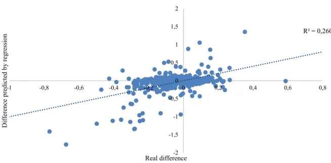
Figure 5: Comparison between the values obtained in regression and real values (ROE)

The figure below presents the regression obtained in Table 4, for Model (I). The dashed line presents the regression line. In the x labels, the actual values for the difference between ROE three years after the IPO and ROE at the IPO year-end. ROE is calculated by dividing the net income by the market capitalization, at the end of the fiscal year. In the y labels, we find the value for the difference between both periods, predicted by the model.

Figure 6: Comparison between the values obtained in regression and real values(ROA)

The figure below presents the regression obtained in Table 4, for Model (II). The dashed line presents the regression line. In the x labels, the actual values for the difference between ROA three years after the IPO and ROA at the IPO year-end. ROA is calculated by dividing the operating income by the market value approximation of cash-adjusted assets, at the end of the fiscal year. Cash-adjusted assets is computed by adding the market capitalization to the book value of assets, deducting the book value of equity and the cash and cash equivalents amount. In the y labels, we find the value for the difference between both periods, predicted by the model.

R² = 0,260 -2 -1,5 -1 -0,5 0 0,5 1 1,5 2 -1 -0,8 -0,6 -0,4 -0,2 0 0,2 0,4 0,6 0,8 Dif fe re nc e pre dicte d by re gre ss io n Real difference

Difference in ROE (IPOyear+3- IPOyear)

R² = 0,259 -2 -1,5 -1 -0,5 0 0,5 1 1,5 2 -1 -0,8 -0,6 -0,4 -0,2 0 0,2 0,4 0,6 0,8 Dif fe re nc e pre dicte d by re gre ss io n Real difference

(25)

4.2. Interpreting the regression models’ coefficients:

An overlook of the two regression models performed led us to assume that both performance indicators are impacted in the same way by the variables selected as independent. In fact, all the variables have the same sign of the coefficients, meaning an increase in the independent variable leads to an increase, if the coefficient is positive, or a decrease otherwise in the performance indicator.

By comparing ROE and ROA as dependent variables, we can assume a positive correlation between them, as they are influenced in the same direction by each variable in the model. To validate this assumption, we computed the correlation between both variables, reaching a value of 0.857. Since this measure scales from -1 to 1, we confirm the stated hypothesis, ROE and

ROA have a strong correlation.

From this point onwards, our analysis will be focused only on the model (I) because studying both regressions would result in redundant conclusions, for the reasons stated above.

4.2.1. Study variable:

The only difference between our treatment and control groups is defined by our study variable

PE_Post. The variable distinguishes the long-term performance between PE-backed IPOs and

others, holding everything else constant.

Being its coefficient significant within a 99% confidence interval, we may conclude on the existence of a PE effect on the long-term performance of IPOs. The surprising effect we did not expect was its negative impact. We were expecting a positive effect of treatment in our sample, as it was the situation found in the Brazilian market (Sincerre, Sampaio, Famá, & Flores, 2019). Another subject these findings contest is the underpricing comparison, leading us to question the investors’ trust in these firms (Lee & Wahal, 2004).

Interpreting the coefficient of the variable PE_Post, we observe a negative influence of PE on the long-term performance of firms, after leaving their ownership. The effect, on average, leads to treated firms obtaining a growth, in absolute measures, of ROE, in three years after the IPO, lower in 7.8% than the control group.

In the following sections, we will identify the main sources of these results, by analysing in-depth the control variables used, in 4.2.2., and effects not detected by the model, in 4.2.3.

(26)

4.2.2. Control variables:

4.2.2.1. Industrial sectors:

The first control variable, from our regression, that was analysed, referred to industrial, two-digit SIC code defined, abnormal performance, IN2D. As the model is centred around its mean, it does not come as a surprise that a variable centred on the average of a sub-group does not have significance for our regression. However, we were still concerned that some industries perform differently than others.

Figure 7: Difference in ROE across sectors

The figure below presents the difference in performance indicator ROE between the year of IPO and three years later by treatment and control groups, represented in the two lines. ROE is calculated by dividing the net income by the market capitalization, at the end of the fiscal year. In the x labels, we may find the name of the industrial sector, ordered by weight in the sample. In the y labels, we find the values for the difference in ROE.

Figure 7 presents the performance of both treatment and control groups across sectors. From this chart, we can conclude that, when firms are PE-backed, they are generally inferior performing than the others. In fact, the ten largest sectors from our sample count for 78% of all observations. From these sectors, PE-backed IPOs are better performing in only two.

In these two sectors, Healthcare Services and Technology Equipment, we find 25 Private-Equity backed IPOs and 16 other firms, summing 9.6% of our sample. These sectors are not representative of the whole market, but its results must be carefully considered, as we may be witnessing strength in previously PE financed IPOs in these segments.

When performing a t-test on the difference in means between both samples, we reject the null hypothesis of the existence of different values for the mean between PE-backed IPOs and others. The p-value was 0.512, leading us reject the null hypothesis of PE-backed firms having a different performance than non-PE-backed, with a 95% confidence level.

-0,55 -0,35 -0,15 0,05 0,25

(27)

4.2.2.2. Leverage:

Changes in leverage (control variable DE) influence negatively the behaviour of ROE in our sample. The regression led us to assume that, when a firm’s debt-to-equity ratio increases by one unit, its expected net income will register a value of 3.5%, as a percentage of shareholders’ equity, lower.

The variable controls for changes in the capital structure of the firms. A second analysis was required to understand if PE-backed IPOs behave differently than others when analysed the leverage ratio at the year-end of the IPO.

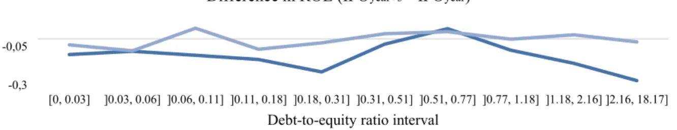
Figure 8: Difference in ROE by the leverage ratio

The figure below presents the difference in performance indicator ROE between the year of IPO and three years later by treatment and control groups, represented in the two lines. ROE is calculated by dividing the net income by the market capitalization, at the end of the fiscal year. In the x labels, we may find ten intervals, each containing 10% of total observations of variable DE at the IPO year. In the y labels, we find the values for the difference in ROE.

The figure above demonstrates that the performance of treated observations is generally inferior to the one of the control group of observations. These conclusions are in line with our regression model.

4.2.2.3. The logarithmic function of assets’ market value:

The variable LA represents changes in the company’s size. The positive coefficient states that, when the size of assets increase by 1%, the ROE is expected to grow by ln(1+1%)*0.127, which is approximately 0.127%.

The model analyses only the changes in total assets, it does not compare the treatment effect among observations with different sizes at the IPO date. To consider this constraint of our model, we present, below, a graphical representation of the long-term performance by the size of the observations at the IPO year-end.

From Figure 9 we conclude that long-term performance has a more accentuated disparity

-0,3 -0,05

[0, 0.03] ]0.03, 0.06] ]0.06, 0.11] ]0.11, 0.18] ]0.18, 0.31] ]0.31, 0.51] ]0.51, 0.77] ]0.77, 1.18] ]1.18, 2.16] ]2.16, 18.17]

Debt-to-equity ratio interval

(28)

have a value for LA at the IPO year-end higher than 14. This fact led us to suspect of abnormal performance effects only for smaller firms.

Figure 9: Difference in ROE by assets’ size

The figure below presents the difference in performance indicator ROE between the year of IPO and three years later by treatment and control groups, represented in the two lines. ROE is calculated by dividing the net income by the market capitalization, at the end of the fiscal year. In the x labels, we may find the value of LA. In the y labels, we find the values for the difference in ROE.

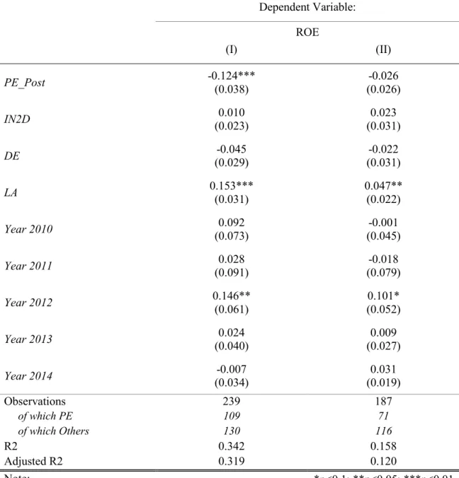
We performed a t-test to the hypothesis of the true difference of means, between control and treated groups, when LA was higher than 14, and conclusions were as follow. With a p-value of 0.210, we rejected the null hypothesis. Having this considered, we decided to create two classes of observations, by their size at IPO year-end: small firms and large firms. Later, we submitted each class to our regression model, defined in Equation (2).

By this second regression, in Table 5, we see that the effect of our variable of study is much more accentuated for smaller firms and that there is no statistical significance for the coefficient of the variable PE_Post in larger firms.

4.2.2.4. Cluster variables (Year):

The use of control variables for the year when IPO was issued allowed us to correct our regression model for economic cycles in the market.

The interpretation of these coefficients states that, holding everything else constant, the average expected difference between ROE in the two periods of study is equal to the beta associated with the year of issue.

The only year cluster coefficient that has significance in our model is the year 2012. Its significance means IPOs issued during this year had a significantly different performance from the rest of the sample. In order to understand if different performances in this year would affect our conclusions, we built two new regressions, in Table 6.

-0,75 -0,5 -0,25 0 0,25 11,5 12,5 13,5 14,5 15,5 16,5 17,5

Logarithm of Assets' Market Value

(29)

Table 5: Regression models by the class of firm size

This table presents the impact of PE-backed IPOs, in comparison to others, on performance measured by ROE. ROE is defined by net income on market capitalisation. Model (I) estimates the Equation (2), with ROE as the dependent variable, for observations categorised as “Small Firms”. Model (II) estimates Equation (2), with ROE as the dependent variable, for observations categorised as “Large Firms”. The regressors are defined as the following. PE_Post is a dummy variable that takes the value 1 for PE-backed IPOs and 0 otherwise. IN2D represents the average value of change of the dependent variable

ROE in the two-digit SIC code industry average, between the year of IPO and three years later. DE is

the change in the leverage ratio, defined through dividing Net Assets market value (assets deducted from market capitalization) by the market capitalization at the end of the fiscal period. LA is a proxy of the changes in the logarithmic function of the total market value of assets’ proxy (book value of assets plus market capitalization at the end of the fiscal period, deducted from the market value of equity). Variables

Year are clustering variables, representing the average difference, in the long-term, of our dependent

variables. Standard errors are presented in parenthesis under the respective coefficient and are transformed in robust standard errors, correcting for homoskedasticity. The symbols *, **, and *** indicate the statistical significance at 10%, 5% and 1% respectively.

Dependent Variable: ROE (I) (II) PE_Post -0.124*** (0.038) -0.026 (0.026) IN2D 0.010 (0.023) 0.023 (0.031) DE -0.045 (0.029) -0.022 (0.031) LA 0.153*** (0.031) 0.047** (0.022) Year 2010 0.092 (0.073) -0.001 (0.045) Year 2011 _(0.091)0.028 _(0.079)-0.018 Year 2012 0.146** _(0.061) _(0.052)0.101* Year 2013 _(0.040)0.024 _(0.027)0.009 Year 2014 _(0.034)-0.007 _(0.019)0.031 Observations 239 187 of which PE 109 71 of which Others 130 116 R2 0.342 0.158 Adjusted R2 0.319 0.120 Note: *p<0.1; **p<0.05; ***p<0.01

(30)

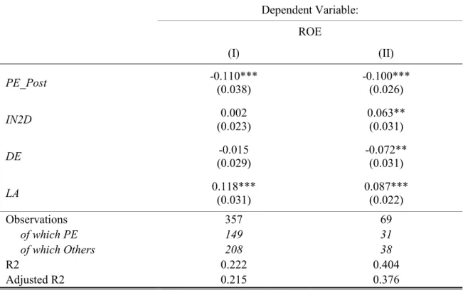
Table 6: Regression models by issue date of IPO

This table presents the impact of PE-backed IPOs, in comparison to others, on performance measured by ROE. ROE is defined by net income on market capitalisation. Model (I) estimates the Equation (2), without year clusters, with ROE as the dependent variable, for observations issued in a year different from 2012. Model (II) estimates the Equation (2), without year clusters, with ROE as the dependent variable, for observations issued in the year 2012. The regressors are defined as the following. PE_Post is a dummy variable that takes the value 1 for PE-backed IPOs and 0 otherwise. IN2D represents the average value of change of the dependent variable ROE in the two-digit SIC code industry average, between the year of IPO and three years later. DE is the change in the leverage ratio, defined through dividing Net Assets market value (assets deducted from market capitalization) by the market capitalization at the end of the fiscal period. LA is a proxy of the changes in the logarithmic function of the total market value of assets’ proxy (book value of assets plus market capitalization at the end of the fiscal period, deducted from the market value of equity). Standard errors are presented in parenthesis under the respective coefficient and are transformed in robust standard errors, correcting for homoskedasticity. The symbols *, **, and *** indicate the statistical significance at 10%, 5% and 1% respectively. Dependent Variable: ROE (I) (II) PE_Post -0.110*** _(0.038) -0.100*** _(0.026) IN2D _(0.023)0.002 0.063** _(0.031) DE _(0.029)-0.015 -0.072** _(0.031) LA 0.118*** _(0.031) 0.087*** _(0.022) Observations 357 69 of which PE 149 31 of which Others 208 38 R2 0.222 0.404 Adjusted R2 0.215 0.376 Note: *p<0.1;**p<0.05;***p<0.01

Analysing the table above lets us be assured that, even though the firms have different performance in the year 2012, it does not change the results obtained with our model. In fact, there is still a similar PE influence present in both groups.

4.2.3. Other factors not captured by the model:

When analysing our sample, we identified two other factors not captured by the model: the firms’ age and the percentage of shares issued at the IPO. As we applied a first differences model, we can only make regressions considering the factors that change between the two times the same firm is observed. Although, performance might also be different for firms with

(31)

different characteristics. As we were able to measure these two factors, we considered them as added value for our understanding of PE effect.

4.2.3.1. Firm’s age:

The age of firms is an important characteristic to bear into consideration (Aldrich & Auster, 1986). To analyse the impact of age on performance, we extracted from Jay Ritter’s website data for the foundation year of each company. Later, we calculated the age at IPO date, resulting in variable Age.

Figure 10: Difference in ROE by age at IPO

The figure below presents the difference in performance indicator ROE between the year of IPO and three years later by treatment and control groups, represented in the two lines. ROE is calculated by dividing the net income by the market capitalization, at the end of the fiscal year. In the x labels, we may find ten intervals, each containing 10% of total observations on variable Age at the IPO year. In the y labels, we find the values for the difference in ROE.

From the figure above we conclude that it is possible that there is no PE effect on firms aged under 6 years. In order to testify this hypothesis, we performed a t-test on the difference in means between the two groups. For the test, we used 150 observations, 45 of which were PE-backed IPOs. The p-value was 0.036, meaning we do not reject the null hypothesis of young firms from the treatment group having worse long-term performance than young firms from the control group, with a 95% confidence level.

All in all, this analysis concluded there is no difference in treatment effect between control and treatment groups. Our regression’s results are not affected by the age of firms at IPO.

4.2.3.2. Percentage of shares issued at IPO:

Equity retention has a positive correlation with performance (Jain & Kini, 1994). A study of the comparison between treatment and control groups, based on the percentage of outstanding shares issued at the IPO, will allow us to verify if it has an impact on the treatment effect. Moreover, it will provide us with the capacity to understand if we can divide our sample into

-0,3 -0,2 -0,1 0 0,1 [0, 1] ]1, 3] ]3, 6] ]6, 7] ]7, 10] ]10, 13] ]13, 18] ]18, 30] ]30, 50] ]50, 148] Age interval

(32)

Figure 11: Difference in ROE by the leverage ratio

The figure below presents the difference in performance indicator ROE between the year of IPO and three years later by treatment and control groups, represented in the two lines. ROE is calculated by dividing the net income by the market capitalization, at the end of the fiscal year. In the x labels, we may find the percentage of outstanding shares issued at the IPO, calculated by dividing the number of shares issued by the total number of outstanding shares on the IPO date. In the y labels, we find the values for the difference in ROE.

From the figure above we suspected on a different influence of treatment in the long-term performance. In fact, the chart indicates that, when equity retention is below 50%, both groups tend to perform more similarly in the long-term.

We performed a t-test to the hypothesis of the true difference of means, between control and treated groups, when the percentage issued was higher than 50%, and conclusions were as follow. With a p-value of 0.153, we reject the null hypothesis. Having this considered, we decided to adopt the same methodology used to investigate firms’ size and created two classes of observations, by equity retention at IPO. Later, we submitted each class to our regression model, defined in Equation (2).

From this model, in Table 7, we concluded that PE-backed IPOs’ performance is also influenced by the percentage of shares issued. However, the variable PE_Post‘s impact was similar in observations with the proportion of issued shares at IPO lower than 50% as in the first model, in Table 4. This created a suspicion on a possible correlation between equity retention and PE backing. When confirming for this relationship, we identified a correlation of -0.224. In fact, these results are aligned with Jain and Kini’s (1994). When firms are PE-backed, they perform worse than others but, these effects are offset by an overperformance registered for firms with higher levels of equity retention. When the percentage of shares issued is higher, the impact of

PE_Post is neglected for two reasons. First, there is a negative impact due to the lower levels

of equity retention. Second, there is a positive impact due to fewer observations of PE-backed in the group. -0,6 -0,4 -0,2 0 0,2 0% 10% 20% 30% 40% 50% 60% 70% 80% 90% 100%

Percentage of Outstanding Shares Issued at IPO

(33)

Table 7: Regression models by the class of firm size

This table presents the impact of PE-backed IPOs, in comparison to others, on performance measured by ROE. ROE is defined by net income on market capitalisation. Model (I) estimates the Equation (2), with ROE as the dependent variable, for observations with the proportion of issued shares at IPO lower than 50%. Model (II) estimates Equation (2), with ROE as the dependent variable, for observations with the proportion of issued shares at IPO higher than 50%. The regressors are defined as the following.

PE_Post is a dummy variable that takes the value 1 for PE-backed IPOs and 0 otherwise. IN2D

represents the average value of change of the dependent variable ROE in the two-digit SIC code industry average, between the year of IPO and three years later. DE is the change in the leverage ratio, defined through dividing Net Assets market value (assets deducted from market capitalization) by the market capitalization at the end of the fiscal period. LA is a proxy of the changes in the logarithmic function of the total market value of assets’ proxy (book value of assets plus market capitalization at the end of the fiscal period, deducted from the market value of equity). Variables Year are clustering variables, representing the average difference, in the long-term, of our dependent variables. Standard errors are presented in parenthesis under the respective coefficient and are transformed in robust standard errors, correcting for homoskedasticity. The symbols *, **, and *** indicate the statistical significance at 10%, 5% and 1% respectively. Dependent Variable: ROE (I) (II) PE_Post -0.080*** (0.026) -0.048 (0.055) IN2D 0.008 (0.019) 0.019 (0.033) DE -0.056 (0.042) -0.020 (0.021) LA 0.162*** (0.031) 0.055 (0.035) Year 2010 0.057 (0.046) 0.036 (0.082) Year 2011 0.074 (0.073) -0.153 (0.123) Year 2012 0.099** _(0.043) _(0.096)0.189* Year 2013 _(0.026)0.017 _(0.042)-0.001 Year 2014 _(0.026)0.036 _(0.033)-0.045 Observations 290 136 of which PE 147 33 of which Others 143 103 R2 0.328 0.233 Adjusted R2 0.309 0.184

(34)

4.3. Findings’ discussion:

In section 4.1. we identified that our treatment group underperformed the control group on both static periods of study. However, as said before, to compare long-term performance we needed more than just identifying two periods. It was required to investigate how each group changed from one situation to another, thus applying the regression model defined in equation (2). The first conclusion drawn from the two first models performed was the positive correlation between the two dependent variables chosen. In fact, positive correlation states that the more effectively the firms’ resources are managed to create profits (ROE), the better performing are its assets to generate operating income (ROA). Both indicators allow the investigator to study operating performance, meaning that, by selecting only one, would result in the same conclusions.

The second conclusion identified in the model overview was the negative, statistically significant, the impact created by the coefficient on the variable PE_Post. This led us to provide some credence to critics of PE. As a matter of fact, measures adopted by these funds may still damage the long-term performance of firms. There is however another possible reason that should not be excluded: investors believe in PE-backed IPOs (Lee & Wahal, 2004).

To investigate if this second justification is aligned with our sample, we performed a t-test to the null hypothesis of having different means of underpricing between treatment and control groups. In fact, with a p-value of 0.0002, we do not reject the null hypothesis. All in all, there is a possibility of PE not being destroying long-term performance, but leading investors to overvalue the firms backed by these funds instead.

We also investigated different factors that could affect performance, concluding that, from our selected control variables, both groups behaved differently under different values for LA. As a matter of fact, when firms are smaller, there is a higher risk of achieving abnormal high or low performance levels. The PE type of funds that focus on growing smaller firms is VC. There might be a different effect of treatment in the long-term performance if all the PE’s types are analysed separately. Leveraged Buyouts, for example, might have a different impact, as these funds invest in usually larger firms (Metrick & Yasuda, 2010). Although, we could not achieve a statistically significant effect on PE_Post for large firms.

The last conclusion we were able to draw was extracted through an analysis of a variable that our regression model could not capture. The larger the portion of shareholders’ equity issued at IPO, the less performing these firms are in the long-term (Jain & Kini, 1994). The treatment

(35)

effect also behaves differently for firms that issue more than 50% of their shares at IPO and the ones that issue less. The latter group is where VC are concentrated, aligning this effect with the conclusions described in the previous paragraph. However, we must bear into consideration that the observations from the former group are only 33 for PE-backed IPOs, which can be another reason for not finding a statistically significant effect on PE_Post for these observations.

4.4. Limitations:

When analysing the findings of our study, one must be aware of its limitations. The conclusions obtained by this investigation are subject to some constraints and further research might provide corrections to them. The main restraints are as follows.

First of all, IPO represents only the third most used exit strategy by LBO funds (Kaplan & Strömberg, 2009). As such, our data is more centred on VC-backed observations, the reason for the control group being more concentrated on smaller firms with lower levels of equity proportion issued at IPO. Further investigation on this topic would require comparing the impacts on long-term performance by each type of PE.

One second constraint is the use of market values, that are subject to being overvalued or undervalued by investors. To improve our conclusions, it is needed to understand whether the negative impact on ROE is created by lower levels of returns or higher values of market capitalisation. This would require a deeper investigation of each firm within our sample. The third limitation identified is the human error, as all our observations were checked individually for the previous relationship with PE funds, available in Thomson Reuters Eikon. Even though our data was carefully treated, one must be aware of this possibility.

Lastly, the sample lacks observations to draw substantiated conclusions on some effects, like the sectorial breakdown, which could identify different impacts on some sectors, particularly in Healthcare Services and on Technology Equipment. Even though it did not have a significant impact, we must consider also the possibility of a different effect of PE financing in these two industrial sectors.

(36)

5. Conclusion:

In this study, we investigated what happened to firms after the exit of PE funds through an IPO. By focusing on the targets’ performance, we seeked to understand, whether supporters of this financing method were right, or if the performance in the price of shares of PE backed companies in the three years following their IPO, is negatively impacted by the incumbrances of having been in a PE fund’s portfolio.

We used a sample of 426 IPOs, 180 of which were PE-backed, from two stock exchanges – NYSE and NASDAQ. We analysed what differed between treatment and control groups in terms of their long-term performance, defined by the three years following the date of listing. We identified that firms with a previous history of PE relationships underperformed the others, in terms of long-term operating performance.

The regression model selected for this thesis was the first differences, as it allowed us to consider variables that did not remain constant throughout the timeline under scrutiny. To evaluate the robustness of our results, we considered different firm-specific characteristics in the IPO year. We evaluated the performance of the Industrial Sectors in which our observations belonged, the size, the leverage ratio, the year of issue, the age and the percentage of equity issued. From these characteristics, we discovered that the treatment effect was not constant when the size and the issued percentage, from shareholders’ equity, were considered. In fact, PE-backed firms are expected to perform poorly, when compared to other firms, especially if the firms are small. For larger firms, we could not achieve a statistically significant result. In what concerns the percentage of shares issued, PE financing only impacts on firms that issued lower percentages of outstanding shares. However, we must consider the possibility of overvaluation of the market capitalization in PE-backed IPOs, as these observations present higher values for underpricing.

All in all, our conclusions raise important managerial questions. Based on our results, managers should be aware of the long-term performance in the value of their companies when financing through PE. Even though PE funds often provide an opportunity for exponential growth, the negative impact, after funds’ exit their investments on the long-term performance, is a cost that must be considered.