Loan modifications and risk of default: a Markov chains approach

(1)

ii

LOAN MODIFICATIONS AND RISK OF DEFAULT: A

MARKOV CHAINS APPROACH

Filipa Cardoso de Almeida

Dissertation presented as the partial requirement for

obtaining a Master's degree in Statistics and Information

Management

(2)

ii

NOVA Information Management School

Instituto Superior de Estatística e Gestão de Informação

Universidade Nova de Lisboa

LOAN MODIFICATIONS AND RISK OF DEFAULT:

A MARKOV CHAINS APPROACH

by

Filipa Cardoso de Almeida

Dissertation presented as the partial requirement for obtaining a Master's degree in Statistics and Information Management, Specialization in Risk Analysis and Management Advisor: Doctor Bruno Miguel Pinto Damásio

March 2020

(3)

iii

ACKNOWLEDGMENTS

The realization of this dissertation would not be possible without the help and support of several people, to whom I would like to leave my most sincere gratitude.

First of all, I would like to thank my advisor, Bruno Damásio, for all the support and accompaniment throughout the development of this work, for all the advice and for always taking me further. A special thanks to Carolina Vasconcelos for the help given in the development of this thesis.

I would also like to thank my friends that accompanied me the most in this journey, Bruna, Luis Miguel, Joana, and Bigo, for all the hours we spent doing work together, studying and also decompressing from all these responsibilities.

A huge appreciation to all my friends who always understood my more considerable absence during the development of this thesis, Inês, Sara, Diogo and Sofia, who listened to me, gave me advice and strengthened me so that this phase of my life resulted with the greatest success.

Last but not least, my most enormous gratitude to my family, for always being there and giving me fundamental support so that I never give up. To my mother, Paula, my sister Beatriz, my aunt and uncle, Carla and Raúl, my grandparents, Conceição and António and my boyfriend, Fábio, thank you, without you none of this would have been possible.

This dissertation marks the end of a phase in my life that, without all of you, would not have been possible to achieve. For this, I leave here my most sincere thanks to all.

(4)

iv

ABSTRACT

With the housing crisis, credit risk analysis has had an exponentially increasing importance, since it is a key tool for banks’ credit risk management, as well as being of great relevance for rigorous regulation. Credit scoring models that rely on logistic regression have been the most widely applied to evaluate credit risk, more specifically to analyze the probability of default of a borrower when a credit contract initiates. However, these methods have some limitations, such as the inability to model the entire probabilistic structure of a process, namely, the life of a mortgage, since they essentially focus on binary outcomes. Thus, there is a weakness regarding the analysis and characterization of the behavior of borrowers over time and, consequently, a disregard of the multiple loan outcomes and the various transitions a borrower may face. Therefore, it hampers the understanding of the recurrence of risk events. A discrete-time Markov chain model is applied in order to overcome these limitations. Several states and transitions are considered with the purpose of perceiving a borrower’s behavior and estimating his default risk before and after some modifications are made, along with the determinants of post-modification mortgage outcomes. Mortgages loans are considered in order to take a reasonable timeline towards a proper assessment of different loan performances. In addition to analyzing the impact of modifications, this work aims to identify and evaluate the main risk factors among borrowers that justify transitions to default states and different loan outcomes.

KEYWORDS

(5)

v

INDEX

1. Introduction ... 1

Background and problem identification ... 1

Study Objectives ... 2

Study Relevance and Importance ... 3

2. Literature Review ... 4

3. Methodology ... 8

Self-Organizing Maps ... 8

3.1.1. Theoretical Framework ... 8

Markov Chains ... 9

3.2.1. Theoretical Framework ... 9

4. Data... 14

Data Set ... 14

Data Preparation ... 16

5. Results and Discussion ... 19

SOM ... 19

5.1.1. Modified Credits ... 19

5.1.2. Unmodified Credits ... 28

Markov Chains ... 39

5.2.1. Modified Credits ... 39

5.2.2. Unmodified Credits ... 43

6. Conclusions ... 52

7. Limitations and Recommendations for Future Works ... 54

8. Bibliography ... 55

9. Appendix ... 58

(6)

vi

LIST OF FIGURES

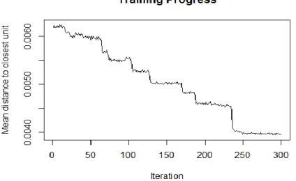
Figure 5.1 - Training Progress of Modified Credits ... 20

Figure 5.2 - Node Counts of Modified Credits ... 20

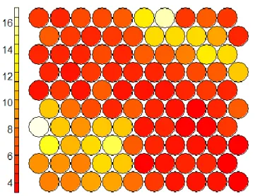
Figure 5.3 - U-Matrix of Modified Credits ... 21

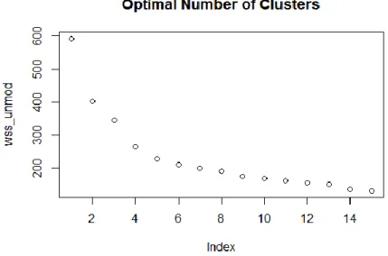
Figure 5.4 - Optimal Number of Clusters of Modified Credits ... 22

Figure 5.5 - Clusters of Modified Credits ... 22

Figure 5.6 - Training Progress of Unmodified Credits ... 29

Figure 5.7 - Node Counts of Unmodified Credits ... 29

Figure 5.8 - U-Matrix of Unmodified Credits ... 30

Figure 5.9 - Optimal Number of Clusters of Unmodified Credits ... 31

(7)

vii

LIST OF TABLES

Table 4.1 - Descriptive Statistics Total Data Set ... 16

Table 4.2 - States of the Markov Chain Methodology ... 18

Table 5.1 - Descriptive statistics (Modified Credits – Cluster 1) ... 23

Table 5.2 - Descriptive Statistics (Modified Credits – Cluster 2) ... 25

Table 5.3 - Descriptive Statistics (Modified Credits – Cluster 3) ... 26

Table 5.4 - Descriptive statistics (Modified Credits – Cluster 4) ... 27

Table 5.5 - Descriptive statistics (Unmodified Credits – Cluster 1) ... 33

Table 5.9 - Transition Probability Matrix (Modified Credits - Cluster 1) ... 39

Table 5.13 - Absorption Probabilities (Modified Credits) ... 42

Table 5.14 - Transition Probability Matrix (Unmodified Credits - Cluster 1) ... 43

Table 5.18 - Absorption Probabilities (Unmodified Credits) ... 46

Table 5.19 - Homogeneity Tests ... 49

Table 9.1 - Mean Absorption Times (Modified Credits) ... 58

Table 9.2 - Mean Absorption Times (Unmodified Credits) ... 58

Table 10.1 - Acquisition Data Elements (source: Fannie Mae) ... 59

(8)

viii

LIST OF ABBREVIATIONS AND ACRONYMS

ANN Artificial Neural Network

BMU Best Matching Unit

CART Classification and Regression Trees

DT Decision Tree

DTI Debt to Income

HAMP Home Affordable Modification Program

HARP Home Affordable Refinancing Program

HOMC Higher-Order Markov Chain

KNN K-Nearest Neighbor

LTV Loan-to-Value

MARS Multivariate Adaptive Regression Splines

MCM Markov Chain Model

MMC Multivariate Markov Chain

REO Real Estate Owned

SOM Self-Organizing Map

SVM Support Vector Machine

TARP Troubled Asset Relief Program

(9)

1

1. INTRODUCTION

B

ACKGROUND AND PROBLEM IDENTIFICATION

Since the period of the global financial crisis that began in 2007, we have been observing an upward concern about credit risk management, as a deficit loan management was one of the central pillars of this crisis. The global financial crisis has brought attention to several areas where there was a need for the improvement of many features, especially in banking management regulation and credit risk management.

Historically, loan modifications were not a very common solution, something that changed with the financial crisis, since during this period there was a considerable increase in the inability of borrowers to repay their loans – in the period that preceded the financial crisis, in the United States, the percentage of non-performing loans was around 1.6%, while at the peak of this financial crisis (around 2010), this percentage increased to about 7.5% (CEIC, 2011). Therefore, loan modifications became a viable solution for banks not to lose the full amount of mortgages, thus promoting repayments by distressed borrowers. Since it is not a recent reality, the studies on loan modifications’ effects are few, making this a significant problem. Furthermore, there continues to exist a large proportion of investigations solely related to the probability of default, essentially a binary analysis, using traditional credit scoring models to attribute classifications on the credit risk level of clients and using linear regression models. However, many issues, as so or even more critical, are fundamental when we discuss credit risk management. These concerns are, namely:

▪ To understand why a customer moves from one state to another;

▪ To assess the probability of a customer going from a state, for example, of delinquency to a normal state, overcoming the difficulty of fulfilling their obligations on credit;

▪ To recognize the best credit conditions for both the bank and the customer, so that the bank guarantees the receipt of all agreed payments and also so that the conditions are not too rigid for the customer;

▪ To notice, if there are modifications at a given moment of the credit, which are the most effective, so that the bank can adapt to such in future contracts and the assessment of the probability of redefault.

The traditional approaches are limited methodologies regarding the determination of transition probabilities. This drawback happens because most methodologies employed do not consider several states and the possible transitions between them. Then, there is a greater concern in determining the risk of a customer entering into default when contracting a loan, depending solely on the customer's profile, traced through its history, that is always required at the time of the contract. Consequently, by discoursing the existence of such states and their possible transitions, there is no concern focused on determining the risk of redefault or even which states influence the transition to that state. The continuity of a loan contract after modifications, triggered by a default event, is a reality. Thus, it is necessary to develop a study focused on the probability of redefault, since the customer's risk profile changes.

(10)

2 A client may reside in more states over the life of a loan than just default. Furthermore, even after a client enters into default, the loan may last after suffering some modifications. In order to properly assess a client’s behavior after loan modifications and thus perform a proper credit risk management, it is necessary to consider the proceeding of loans. Even though various methods, such as linear regression, allow to model several states of categorical variables, these can not capture the entire probabilistic structure of the process in the case where the mean is not linear. Hence, a discrete-time Markov chain is considered. Several states and transitions between those states are taken into account, describing all the possible situations in which a loan can be in, allowing the establishment of credit risk based on behavioral aspects. This way, we are able to incorporate historical information in the assessment of the probability of redefault, capturing the occurrence of all states occupied by a client.

S

TUDY

O

BJECTIVES

The main goal of this study is to evaluate the impact of the modifications in loans in order to determine if those modification are effective, i.e., if they reduce the probability of a borrower to default. This assessment becomes essential as a credit risk management tool because it will allow us to determine whether these changes are, in fact, able to be used to mitigate risk in financial institutions, therefore having a considerable impact in the banking business, as well as a significant influence on the life of borrowers. This ambition requires an analysis of the variables influencing several groups of clients, with similar characteristics. Those groups will be constructed through cluster, using Self-Organizing Maps (SOMs). With this, we will then be able to compare groups of clients, instead of comparing individual clients.

Considering the goal of this work, we will focus on the loans’ performance data. We will use a discrete-time Markov chain model (MCM) to estimate the probabilities of transitioning from one state to another, relying on the Transition Probability Matrix (TPM) to calculate the probability of default. Following this rationale, we can also evaluate how the modifications of the various states of a loan influence the probability of default considering the history of clients.

Furthermore, in order to achieve the main objective of this dissertation, we aim to compare the probability of default before the modifications and the probability of default after the modifications. For the first group of loans, we will limit our data to loans that never defaulted and estimate their corresponding TPM. For the second group of loans, we will solely consider loans which conditions were modified and estimate their corresponding TPM. Therefore, we can infer if the modifications are effective. Additionally, we will evaluate the impact that different loan performances have in the probabilities estimated as well as link the different risk factors to the different performances of individuals.

(11)

3

S

TUDY

R

ELEVANCE AND

I

MPORTANCE

Credit risk models are a critical tool in risk management and credit risk management is one of the major concerns of banks, since loans are one of the main bank’s products. Therefore, the development of several studies on the best method of credit risk assessment is reasonable, as well as a growing attempt to find a method that fits better than the existing ones.

Most investigations are mainly concern with credit risk modelling in several types of loans such as consumer loans, credit card loans and mortgages. The most common credit-scoring methodology, the logistic regression model does not allow an evaluation of the client’s behavior between non-default and default states. Hence, it is possible to infer that this model only concerns with the transition to a default state from a non-default state. Additionally, multinomial methodologies are other comprehensively applied strategies in which several states are predominantly considered. However, they impose a functional form, only modeling the conditional mean. This limitation started to be widely recognized, so the adoption of other methodologies was found to be necessary. The MCM has proven to be a very efficient solution when it comes to evaluating the behavior of a client over the life of a loan. Some examples of studies using Markov Chains are those of Régis, D. E. & Artes, 2016, to identify credit card risk and Leow, M. & Crook, J. 2014, in which the MCM was used to predict the probability of credit card default to estimate the probability of delinquency and default for credit cards. Betancourt, L. 1999, applied MCM to estimate losses from a portfolio of mortgages, and therefore, estimate the accuracy of Markov chain models on mortgage loan losses. Chamboko, R. & Bravo, J. M 2016, utilized MCM as a tool to model transition probabilities between the various states and estimating the probability of loans transitioning to and from various loan outcomes and acquisition and performance explanatory variables. Malik, M. & Thomas, L.C. 2012, among others, tested MCM to estimate consumer credit ratings and to model retail credit risk.

As we can see, using Markov chains model is advantageous when we want to describe the dynamics of credit risk, since it focusses on transition probabilities between different states. Consequently, this methodology is very valuable to model credit risk, emphasizing the use of transition probabilities to determine the probability of default. However, these studies do not extend to the probability of redefault, which becomes a reality and a source of alarm since loan modifications are a recent solution in credit risk management. For this reason, the development of this study is critical to fulfilling this gap. The discrete-time Markov chain model circumvents the use of simplified approaches, considering the states and transitions that occur during the lifetime of a loan. In this research, we will only consider long-term loan data, so that sufficient time for analysis is provided. In a simplified approach, just two states and one type of transition are considered – states of default and non-default and the transitions to one another. Several states, such as delinquency, recovery, short sale, prepayment, among others, are considered in the discrete-time Markov model. Subsequently, we can calculate transitions and respective probabilities between all states.

The great advantage of this methodology is that we are able to model the entire probabilistic structure of a process, capturing complex and less noticeable relationships. Moreover, unlike traditional parametric methods, not only nonlinearities at the conditional mean, but also higher moments of the distribution of a process are taken into account.

(12)

4

2. LITERATURE REVIEW

Credit is one of the main products of banks, so it is necessary to implement extremely rigorous and careful management to be closer to the needs of banks, as well as the needs of clients. It is fundamental to model credit risk so that banks are capable of adapting to some eventual modifications that occur over time, especially in the event that clients do not comply with their credit obligations. This need is clearly recognized, and therefore credit risk models have been used for a long time, being a subject of research over the last 50 years. As a result of credit risk models being an important matter of study, several models apply not only to credit risk in mortgages but also to consumer credit risk, credit cards, among others. Consequently, several credit risk models were developed.

As previously stated, loan modifications started to become more common with the 2007 financial crisis. Throughout this crisis, it is possible to identify various socioeconomic aspects that have markedly influenced some behaviors. This global crisis has led to a deterioration of economic conditions, particularly a large increase in unemployment, which is one of the factors that most affects an individual’s capacity to cope with his expenses, particularly when borrowing, following income, cashflow and liquidity shocks. There are also other social factors such as divorces or other casualties from the social forum, that lead to health degradations which, in turn, can lead to more serious situations that have a negative consequence when these individuals have commitments with banks. Nevertheless, numerous aspects beyond the conditions of the loans themselves, should also be carefully analyzed. These elements include the rigidity of mortgage contracts, some default trigger events such as high house prices, interest rates and borrowers’ credit history, which are essential to consider.

Additionally, there are other concepts that we must include when we analyze the course of loans, such as strategic default, that happens when a borrower chooses to default despite having enough monetary funds to continue to pay the mortgage. Also, the incorporation of several states, like “delinquency” – a pre-default state –, “foreclosure” – the bank takes control of a property, expels the householder and sells the home after the householder is incapable fulfilling his mortgage as specified in the mortgage contract – and “cure” – recovery from delinquency state. This complexity of characteristics worthy of analysis converts into the necessity to find the methods that best fulfill this objective. Accordingly, we can observe the development of several different studies and methodologies capable of supporting such complexity.

Altman (1968) proposed a discriminant analysis to determine combinations of observable characteristics, i.e., the contribution of each explanatory variable, to assess the probability of default. This credit scoring model is widely recognized as the “Z-Score Model,” which uses financial ratios to predict corporate bankruptcy by attributing a Z-Score1_{to an obligor. The author concluded that}

companies with a Z-Score below 1.81 go bankrupt, while companies with Z-Scores above 2.99 do not fall into bankruptcy. For Z-Scores between those two values, it is considered a “zone of ignorance,” where we cannot accurately determine whether the company falls into bankruptcy. Following this proposed methodology, many models based on credit scoring appeared with important contributions

(13)

5 to credit risk analysis. The most well-known models in this area, therefore being the most applied when it comes to credit scoring, are the Regression Models. Within Regression Models, we have Logit Models (Martin, 1977) and Probit Models (Ohlson, 1980). As previously mentioned, these models are quite adequate in credit scoring. However, these methodologies only focus on the probability of default in order to perform credit scoring studies, being simple probabilistic formulas for classification and, therefore, not capable to accurately deal with nonlinear effects of explanatory variables.

In the meantime, other models that fulfill more complex needs emerged, such as machine learning models. An example is the machine learning classification technique named K-Nearest Neighbors (KNN). Chatterjee and Barcun (1970) first applied the nearest neighbor to credit risk evaluation. Years later, Henley and Hand (1997) considered the development of a credit scoring system using KNN methods. These strategies are non-parametric, whose algorithm analyzes patterns of the k-nearest observations that are most identical to a new observation. KNN methods can be applied to classification and regression predictive problems, frequently being employed for its easy interpretation and short calculation time. Other simple and easily understandable models, such as Decision Trees (DT), can also be applied as credit risk models. A decision tree consists of a non-parametric approach of nodes and edges, mapping observations of an individual to make conclusions about the individual’s class. It is constructed automatically by a specific training algorithm employed on a given training dataset. DT models are frequently used together with other methods, such as a rule draw, to interpret some complex models, like artificial neural networks (ANN). ANN are computational methods that replicate the human brain’s way to process information so that one may identify the client’s characteristics that, in the credit scoring area, are related to the default event, enabling to determine which characteristics influence the different types of clients. An example of this combination between DT and ANN is the use of DT to visualize the credit evaluation knowledge extracted from neural network on a credit dataset, by Baesens et al. (2003) and Mues et al. (2006).

Classification and Regression Trees (CART), defined as a decision tree graphic that classifies a dataset into a finite number of classes, is a methodology used in credit risk as well. Furthermore, there are Hybrid Methods (Zhang et al. 2008) that combine one or more methods, as in the case with DT and ANN. Several experiments have demonstrated that using two or more single models can generate more accurate results by overcoming weaknesses and assumptions of a single method and therefore produce a more robust forecasting system. As was recognized, there are great benefits in using hybrid methods. Two typical hybrid methodologies commonly used in credit risk, such as Support Vector Machines (SVM), an optimization method, and machine learning procedure, which was first proposed by Vapnik (1995), has the minimization of the upper bound of the generalization error as its main idea. Freidman (1991) proposed a non-linear parametric regression known as Multivariate Adaptive Regression Splines (MARS).

As mentioned previously, studies on credit risk management models fostered the exploration of the most appropriate model and also an examination of which model best overcomes the limitations of other methodologies. Furthermore, following the financial crisis that began in 2007, we have been observing an increasing number of researchers dedicated to analyzing several factors as determinants for events such as default and foreclosure. This circumstance is also why hybrid models emerged. In the last few years a new type of methodology, Survival Analysis, was developed. Survival models have

(14)

6 been pointed out as preferable to other models due to their ability to incorporate variations in the credit over time that affect performance on the loan payment and the ability to forecast the occurrence of events (default, recovery, prepayment, foreclosure). Survival models have been frequently used to model the risk of default (Bellotti and Crook 2013; Noh et al. 2005; Sarlija et al. 2009; Tong et al. 2012), but also to model foreclosure on mortgages (Gerardi et al. 2008) and to model recovery from delinquency to current or normal performance (Ha 2010; Ho Ha and Krishnan 2012; Chamboko and Bravo 2016).

Although all these models have their advantages and disadvantages, it is essential to mention that the vast majority consist of two-state credit risk models. The problem with such models is that they tend to disregard the transition behavior between other states beyond just default and no default. Accordingly, multi-state models emerged, providing an answer to this limitation. Multi-state models (Hougaard, P. 1999) are models for a process, such as describing the life history of an individual, which at any time occupies one of a few possible states, thus allowing the modelling of different events as well as intermediate and successive events. Multi-state models are mostly interpreted as Markov models considering that these models acknowledge several states as well as the transitions between them, therefore allowing the calculation of the probability of transition between events through the earlier discussed TPM. Trench et al. (2003) created a Markovian decision-making method to lead a bank to identify the price of credit card owners in order to improve their profits. Additionally, this methodology was also used in revolving consumer credit accounts, influenced by the consumer’s behavior as well as the impact on the economy of that behavior. Furthermore, Malik and Thomas (2012) conceived a Markov chain model based on developmental results to determine the credit risk of consumer loan portfolios.

In summary, multi-state models can assume different states through time. Most commonly, the Markovian assumption is adopted. In the particular case of loans, Markov chains helps to describe the dynamics of credit risk, since they estimate transition probabilities between different states. Nonetheless, Markov Models do not exclusively apply to credit studies. In fact, MCM have the most wide-ranging of applications. One of the most widely known case of Markov chains’ application is Google’s PageRank (Page, L., et al., 1998). This element shows us that this methodology can also be used in the world of computing and programming (to program algorithms) and computer science – randomized algorithms, machine learning, program verification, performance evaluation (quantification and dimensioning), modeling queuing systems and stochastic control.

As a statistical model, Markov chains have many applications in the real world, with such a wide range ranging from music (Volchenkov, D. & Dawin, J. R., 2012), to linguistics (Markov, 1913), finance (Siu et al., 2005; Fung and Siu, 2012), to the estimation of option prices (Norberg, R., 2003) and financial markets (Maskawa, 2003; Nicolau, 2014; Nicolau and Riedlinger, 2015), economics (Mehran, 1989), economic history (Damásio and Mendonça, 2018), operational research (Asadabadi, 2017; Tsiliyannis, 2018; Cabello, 2017), management (Horvath et al., 2005), forecasting (Damásio and Nicolau, 2013) and sports (Bukiet et al., 1997). They are also used in medicine (Li et al., 2014), biology (Gottschau, 1992; Raftery and Tavaré, 1994; Berchtold, 2001), such as DNA sequences and genetic networks, physics (Gómez et al., 2010; Boccaletti et al., 2014), astronomy and environmental sciences (Turchin, 1986; Sahin and Sen, 2001; Shamshad et al., 2005). Regarding the engineering area, Markov chains have been

(15)

7 used in chemical engineering (to predict chemical reactions), physical engineering (to model heat and mass transfers), and aerospace. Indeed, most population models are Markov chains – they are used when we want to know how population changes over time or when we want to estimate the probability that a population, animal or plant, may be extinct.

The extensive use of Markov chains shows the great utility that this methodology has, not only within the applied mathematics area but also in most scientific areas. This versatility proves that a model that was first published in 1906 continues to be a handy and efficient tool in the most varied scientific aspects.

(16)

8

3. METHODOLOGY

In order to achieve the objective of this dissertation, we propose the application of an innovative hybrid methodology in the evaluation of the performance on loans, i.e., a new multidisciplinary combination of two distinct methodologies in this subject. These two methodologies consist of a clustering technique named Self-Organizing Maps (SOMs) and the application of the Markov Chains methodology. The application of the first methodology – SOM – will be the basis for the second and principal methodology – Markov Chains.

Fannie Mae’s Single-Family Loan Performance Data is the data source employed in this study. This data comprises both borrower and loan information at inception, as well as performance data on loans. R software will be used to accomplish the main objective of this work.

S

ELF

-O

RGANIZING

M

APS

SOMs were introduced by Teuvo Kohonen (1982) and are a class of artificial neural networks that use unsupervised learning2_{neural networks for feature detection in large datasets, identifying individuals}

with similar characteristics, organizing and gathering them by groups or clusters. This approach contrasts with other artificial neural networks, since they apply competitive learning3_{instead of}

error-correction learning4_.

A SOM comprises neurons in a grid, which iteratively adapt to the intrinsic shape of our data. The result allows us to visualize data points and identify clusters, being used to produce a low-dimension space of training samples. Therefore, its main objective is to reduce the dimensionality of data, performing a discretized representation of the continuous input space, where there are the initial dataset and the input vectors – lines of the matrix of observation –, named map. The reduction of dimensionality then occurs in the nodes or space where the vectors will be projected.

3.1.1. Theoretical Framework

The SOM algorithm follows five steps. Initially, we have an input space, 𝑋 ∈ ℛ𝑛. At the start of the learning, each node’s weight, {𝑤1, 𝑤2, … , 𝑤𝑀} is initialized, where 𝑤𝑖 is the weight vector associated

with each neuron, and M is the total number of neurons. Next, one data point is chosen randomly from the dataset, and then every neuron is examined to calculate which one’s weights are more similar – and, therefore, closest – to the input vector. The winning node is known as the Best Matching Unit (BMU)5_{. The BMU is moved closer to the randomly chosen data point– the distance moved by the BMU}

is determined by a learning rate, which decreases after each iteration. The BMU’s neighbors are also

2_{Unsupervised learning means that we only have input data and no output variables, contrasting with}

supervised learning, where input data and output variables are given.

3_{Competitive learning is a form of unsupervised learning artificial neural networks where, given the input,}

nodes compete with each other to maximize the output.

4_{Error-correcting learning is a type of supervised learning where we compare the system output with the}

desired output value and use that error (the difference between the desired and obtained values) to direct the training.

5 _{BMU is a technique which calculates the distance from each weight to the sample vector, by running}

through all weight vectors. The weight with the shortest distance is the winner. The most commonly way used to determine that the distance is the Euclidean distance.

(17)

9 moved closer to that data point, through a neighborhood function, with farther away neighbors moving less. Finally, these steps are repeated for N iterations.

Succinctly, at each time 𝑡, present an input 𝑥𝑡, and select the winner, such as

𝜈(𝑡) = 𝐵𝑀𝑈 = arg 𝑚𝑖𝑛𝑘𝜖Ω‖𝑥𝑡− 𝑤_𝑘𝑡‖ (3.1)

where ‖𝑥𝑡− 𝑤_𝑘𝑡‖ is the Euclidean distance.

Weights are adjusted after obtaining the winning neuron until the map converges to increase the similarity with the input vector. The rule to update the weight vector is given by

∆𝑤𝑘(𝑡) = 𝛼(𝑡)𝜂(𝜈, 𝑘, 𝑡)[𝑥𝑡− 𝑤_𝜈𝑡] (3.2)

where coefficient 𝛼𝑡 𝑖𝑠 the previously mentioned learning rate and 𝜂(𝜈, 𝑘, 𝑡) if a neighbor function.

The use of the SOM methodology becomes very interesting and useful because it allows us to map the input data, that is, it permits us to allocate customers to a particular group, with each group from the beginning, with each group formed containing customers with similar characteristics. This aspect proves to be quite advantageous not only for this study, since it facilitates the interpretation and evaluation of our data, but it is also a tool with great added value for banks since it allows them to replicate the same procedure in their business with new and ongoing customers. In such a way, it allows them to understand the profile of each customer in advance and thus make an initial forecast of the future behavior of those same customers, comparing them with others in the same group. Since we have an extensive dataset, we can see that this methodology becomes quite useful in our case. Additionally to what was previously mentioned, the SOM methodology reveals to be a useful approach because it is a numerical and non-parametric method as well as a methodology that does not need a priori assumptions about the distribution of data and a method that allows the detection of unexpected characteristics in the data because of its use of unsupervised learning. The application of the SOM methodology makes it is possible not only to reduce the dimensionality, but also to organize the data. That is why its interpretation is simpler. This first methodology will allow the identification of comparable clients, let us say, with the same loan maturity, with the same interest rate or which performed the same statuses. Considering that the result of the application of this methodology is the organization of data in clusters that contain groups of clients with similar characteristics, we will then be able to compare groups of clients, instead of comparing individual clients. Additionally, it also makes it easier to apply Markov chains, since it allows the implementation of a Markov chain on each cluster.

M

ARKOV

C

HAINS

3.2.1. Theoretical Framework

3.2.1.1. First Order Markov Chains

The Markov chain is named after the well-known Russian mathematician Andrey A. Markov (1856-1922), distinguished for his work in number theory, analysis, and probability theory. He lengthened the weak law of large numbers and the central limit theorem to a specific series of dependent random

(18)

10 variables. Accordingly, he created a special class, denominated Markov processes: random processes in which, given the present, the future is independent of the past. Therefore, a Markov chain is a Markov process defined into a countable state space. This factor means that the probability that the process will be in a given state at a given time 𝑡 may be deducted from the knowledge of its state at time 𝑡 < 𝑡𝑡−1 and does not depend on the history of the system before 𝑡.

Consider the stochastic process

{𝑋_𝑡, 𝑡 = 0, 1, 2, … } (3.3)

That takes discrete-time values at any time point 𝑡:

𝑋𝑡 = 𝑗 , 𝑗 = 0, 1, 2, … (3.4)

in which 𝑗 represents the state of the chain.

Without any loss of generality, to ease the notation we assume 𝑀 to be finite, as follows:

𝑀 = {1, 2, … , 𝑚} (3.5)

For the discrete-time context, we can conclude the present state 𝑋𝑡 is independent of past states, such

that:

𝑃(𝑋𝑡= 𝑗 | 𝐹𝑡−1) = 𝑃(𝑋𝑡 = 𝑗 | 𝑋𝑡−1 = 𝑖) (3.6)

where 𝐹𝑡−1 is the 𝜎 − 𝑎𝑙𝑔𝑒𝑏𝑟𝑎 generated by the available information until 𝑡 − 1.

Considering that we can calculate the probability of a state transiting to the next state – transition states –, we can then call this a transition probability. Hence, it is possible to construct a transition probability matrix (TPM): [ 𝑃(𝑋𝑡 = 1|𝑋𝑡−1 = 1) ⋯ 𝑃(𝑋𝑡 = 𝑚|𝑋𝑡−1= 1) ⋮ ⋱ ⋮ 𝑃(𝑋𝑡 = 1|𝑋𝑡−1 = 𝑚) ⋯ 𝑃(𝑋𝑡 = 𝑚|𝑋𝑡−1 = 𝑚) ] (3.7)

This operation is denominated the one-step transition probability matrix of the process. Additionally, we can also calculate the probability that the chain will visit state 𝑗 after n-steps given the fact that it was in state 𝑖 at time 𝑡 − 1. Thus, we have the n-step transition matrix, 𝑃𝑛, in which 𝑃 is the one-step transition probability matrix and 𝑃𝑛 is equal to 𝑃 × 𝑃 𝑛 times.

One of our objectives is to describe how the process travels from one state to another in time. Then we have:

𝑃(𝑋𝑡 = 𝑗 | 𝑋𝑡−1 = 𝑖) (3.8)

We are mostly concerned in how Markov chains evolve in time. From that point of view, there are two types of behaviors that are important to highlight: (i) transient behavior, which describes how chain moves from one state to another in finite time steps; and (ii) limiting behavior, which defines the behavior of 𝑋𝑛 as 𝑛 → ∞. Thus, it is fundamental to define some concepts:

(19)

11 ▪ For every state 𝑖 in a Markov Chain, let 𝑓𝑖 be the probability that beginning in state 𝑖, the

process will ever re-enter state 𝑖.

▪ State 𝑖 is said to be recurrent if 𝑓𝑖= 1 and transient if 𝑓𝑖 < 1, i.e., if the probability is different

from 1.

▪ A recurrent state is said to be positive if its mean recurrence time6_{is finite and is aided to be}

null if its mean recurrence time is infinite. Consequently, an irreducible7_{Markov chain is}

positive recurrent if all its states are positive recurrent. Positive recurrent irreducible Markov chains are often called ergodic.

A Markov Chain with a finite state space 𝑀 is said to have a long-run distribution, i.e., a limit distribution if

lim

𝑛→∞𝑃(𝑋𝑡+𝑛 = 𝑎| 𝐹𝑡−1) = 𝜋𝑎 (3.9)

As previously mentioned, a Markov Chain is said to be ergodic if it is positive recurrent and aperiodic. Under these conditions, we have the following equation:

𝜋𝑃 = 𝜋, 𝑤𝑖𝑡ℎ ∑ 𝜋𝑖 = 1 𝑎𝑛𝑑 𝜋𝑖 ≥ 0 𝑚

𝑖=1

(3.10)

where P is the PTM associated with the Markov Chain. Therefore, for any 𝑛 ≥ 1, we have:

𝜋𝑖 = 𝑃(𝑋𝑡 = 𝑖) (3.11)

3.2.1.2. Absorbing Markov Chains

A Markov chain is absorbing if it has at least one absorbing state, and if from every state it is possible to go to an absorbing state. A state 𝑖 of a Markov chain is called absorbing if it is impossible to leave it (Grinstead, C. M & Snell, J. L. 1999), such as:

𝑃(𝑋𝑡 = 𝑖 | 𝑋𝑡−1 = 𝑖) = 𝑃𝑖𝑖 = 1 (3.12)

When a Markov chain process attains an absorbing state, we must denominate it absorbed. By opposition, a state which is not absorbing is called transient, a definition that was previously provided. Consider an arbitrary absorbing Markov chain. Now reorder the states so that the transient states come first. With 𝑡 transient states and 𝑟 absorbing states, the transition matrix 𝑃 can be written in the following canonical form:

𝑃 = (𝑄 𝑅

𝟎 𝐼) (3.13)

6_{Mean recurrence time is the average time it requires to visit a state 𝑖, starting from 𝑖.}

7_{A Markov chain is said to be irreducible if all states belong to the same class. State 𝑖 and state 𝑗 are said}

to communicate if state 𝑖 and state 𝑗 are accessible (starting from state 𝑖, it is possible to enter state 𝑗 in future number of transitions) (Ching, W. & Ng, M., 2016).

(20)

12 where 𝐼 is an 𝑟-by-𝑟 identity matrix, 𝟎 is an 𝑟-by-t zero matrix, 𝑅 is a nonzero 𝑡-by-r matrix, and 𝑄 is a 𝑡-by-𝑡 matrix. The first 𝑡 states are transient and the last 𝑟 states are absorbing.

For an absorbing Markov chain, the matrix 𝐼 − 𝑄 has an inverse 𝑁 matrix, called the fundamental

matrix. The entry 𝑛𝑖𝑗 of 𝑁 gives the expected number of times that the process is in the transient state

𝑗 if it is started in the transient state 𝑖. The decomposition of the transition matrix into the fundamental matrix allows for certain calculations such as the mean time of absorption, i.e., the mean number of steps until absorption from each state. Accordingly, the fundamental matrix 𝑁 can be written as follows:

𝑁 = (𝐼𝑡− 𝑄)−1 (3.14)

where 𝐼𝑡 is a 𝑡-by-𝑡 identity matrix.

Additionally, it is possible to define the time of absorption as follows. Let 𝑡𝑖 be the expected number

of steps before the chain is absorbed, given that the chain starts in state 𝑖. Now let 𝑡 be the column vector whose 𝑖th entry is 𝑡𝑖. Then,

𝑡 = 𝑁𝑐 (3.15)

where 𝑐 is a columns vector whose entries are 1.

Furthermore, it is possible to define the probability of absorption8_{by a specific absorbing state when}

the chain starts in any given transient state. Let 𝑏𝑖𝑗 be the probability that an absorbing chain will be

absorbed in the absorbing state 𝑗 if it starts in the transient state 𝑖. Now let 𝐵 be the matrix with entries 𝑏𝑖𝑗. Then 𝐵 is a a 𝑡-by-𝑡 matrix and

𝐵 = 𝑁𝑅 (3.16)

Where 𝑁 is the fundamental matrix and 𝑅 is as in the canonical form.

Now that a brief theoretical framework of absorbing Markov chains was provided, it is possible to verify that, with the application of the proposed hybrid methodology, the estimation of the probability of absorption as well as the estimation of the mean absorption time, we will be able to perform an important comparison between the different types of credit (modified versus unmodified), as well as a comparison between the clusters calculated within of each type of credit, regarding two specific states, that we will address later.

The main objective of this work is to evaluate, based on the results obtained from the proposed hybrid methodology, if the loan modifications are, in fact, effective. For that, we will estimate the probability of client defaults considering unmodified loans and the probability of default considering modified loans whereby the terms of the contract are altered. To that end, we will stack individuals and eliminate spurious transitions, that is, transitions between individuals and, therefore, between credits.

8_{Given a transient state 𝑖 we can define the absorption probability to the recurrent state 𝑗 as the probability that}

the first recurrent state that the Markov chain visits (and therefore gets absorbed by its recurrent class) is 𝑗, 𝑓𝑖∗𝑗

(21)

13 Thus, we will be able to estimate the transition probabilities based on the performance of each individual.

By applying a Markov chain on each cluster obtained from the application of the SOM methodology, we will estimate a TPM for each cluster built for unmodified modified credits, considering the respective loan modifications. The objective is to compare the estimated TPMs and evaluate the differences between modified and unmodified credits. Therefore, we are able to evaluate if the modifications are, in fact, effective and what modifications are most efficient.

The use of these two methodologies together has proven to be quite useful in other studies outside the financial scope. A hybrid approach combining a SOM and a Hidden Markov Model (HMM) was previously used to meet the increasing requirements by the properties of DNA, RNA and protein chain molecules (Ferles, C. & Stafylopatis, A. 2013), as well as an application concerning o stroke incidence (Morimoto, H. 2016). Additionally, it was adopted as a hybrid methodology to forecast the influence of climatic variables (Sperandio, M, Bernardon, D. P. & Garcia, V. J. 2010), to test speech recognition (Somervuo, P. 2000) and also to analyze career paths, as a study to evaluate the insertion of graduates and to identify the main career paths categorizations (Massoni, S., Olteanu, M & Rousset, P 2010). Although the hybrid use of these methodologies has been implemented in other areas, its use in financial and banking areas represents an interdisciplinary innovation. Thus, not only is it presented as a methodology that simplifies the interpretation and processing of data, but also as an innovative approach.

(22)

14

4. DATA

D

ATA

S

ET

The primary dataset used in this study is Fannie Mae’s Single-Family Loan Performance Data, that provides data on US mortgages purchased from original lenders. The Single-Family Fixed-Rate Mortgage (primary) dataset contains a subset of Fannie Mae’s 30-year and less, fully amortizing, full documentation, single-family, conventional fixed-rate mortgages (Fannie Mae, 2019).

We will analyze a total of 149 404 loans acquired by Fannie Mae in 2006, divided into 40 079 modified credits and 109 325 unmodified credits, following their performance until 2015. This timespan is an interesting period to evaluate, since there was an economically and financially critical period that, as previously mentioned, began in 2007. We are then able to track loans that were purchased in the pre-crisis period and evaluate their development through the pre-crisis period and the post-pre-crisis period. Hence, it is interesting to evaluate these 10 years, since it is transversal to several scenarios that occurred during this time.

The financial crisis occurred all over the world, and it is noteworthy to evaluate, especially in the United States. During this period, some remarkable events occurred, such as the collapse of Lehman Brothers and also significant changes in monetary policies. This cataclysm led to historically low-interest rates and the approval of two large-scale debt relief programs – the Home Affordable Refinancing Program (HARP) and the Home Affordable Modification Program (HAMP) – along with the foundation of the Troubled Asset Relief Program (TARP).

The population data is divided into quarters, and for each quarter, we have a division in “Acquisition” and “Performance” datasets. We can assess the full history of the contracts in each quarter which means that it does not represent a three-month observation of the mortgages. The “Acquisition” dataset has the information on the origination of the credit and the “Performance” dataset has the full credit information related to its evolution, having a Loan Identifier (ID) that links the “Acquisition” dataset to the “Performance” dataset. In this way, we ensure that the subsequent performance of a loan can be monitored from the outset, therefore allowing the modelling of the various loan outcomes. The “Acquisition” data includes static data on both borrower and loan information at the time of origination. This information comprises the Acquisition Data elements, such as the Interest Rate, the Loan Amount, the Number of Borrowers, the Borrower Credit Score, and the Loan Term. The “Performance” data includes the proceeding of loans from the time of the acquisition up until its current status. This dataset is segregated in months and displays the loan performance characteristics, since it considers a dynamic performance over time. The information that follows the behavior of the clients is contained in the Performance Data Elements, such as the Current Loan Delinquency Status, the Zero Balance Code, the Current Interest Rate and the Modification Flag. Further details on these data elements are available in Table 10.1 and Table 10.2 presented in the annexes.

Some variables were modified in order to allows us to apply the previously described SOM methodology and also to be more adequate for our analysis. Later, in section 4.2., we will outline the variables considered in this study as well as the ones that were modified. A description of those modifications and the reasoning behind it will also be provided.

(23)

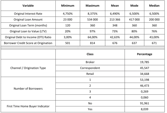
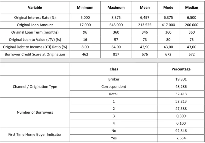
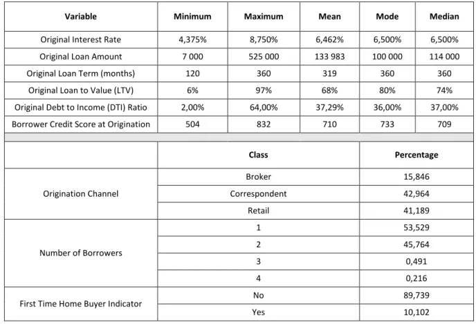
15 Before we go further in this study, i.e., before we develop the SOM and Markov chain methodologies, it is fundamental to analyze the global data set. This analysis will allow us to understand its composition before segmenting it into modified and unmodified credits as well as to assess the disparity of each credit class – modified or unmodified – in relation to the entire data set. Accordingly, in Table 4.1 we present the descriptive statistics, as well as a complementary analysis of these results.

By analyzing the descriptive statistics, we can observe that about 10% of the individuals were first time home buyers, with the majority of the contracts owned by one borrower (about 53%), even though a considerable percentage of the contracts were owned by two borrowers (about 46%). Additionally, most of the contracts were originated by correspondent lending, which is the process through which a financial institution underwrites mortgage loans using its own capital. Nevertheless, a considerable segment of the contracts was purchased through retail lending, i.e., it is based on lending to individual or retail customers, most often by banks, and institutions focused solely on the credit business. Furthermore, the interest rate of the contracts under analysis range from 3,000% to 10,950% with a mean of 6,470% and a mode of 6,500%. Regarding the loan amount, we have a range from $7 000 to $802 000 with a mean value of $155 449 and a mode of $100 000. Most of the contracts have a duration of 360 months, which corresponds to 30 years. This scenario is typical since we are considering mortgage loans, which are usually very long-term contracts.

Regarding the risk characteristics of the individuals, we have the LTV ratio, the DTI ratio, and the Borrower Credit Score. The LTV ratio corresponds to the percentage of the property value that the loan covers, which means that if we have an LTV ratio of 70% it indicates that the loan covers 70% of the property appraisal value. Therefore, the higher the amount borrowed, the greater the risk the bank takes, since it means that the bank lends a larger amount of money. In fact, in some situations, derived from the high risk taken by the bank, it may require the borrower to purchase mortgage insurance to offset that risk. In the data set under study, we have an LTV ratio between 1% and 97% with a mean value of 7% and a mode of 80%. Although most banks only allow a loan that corresponds to a maximum of 80% of the property appraisal value, in our case study, we have values of 97% because Fannie Mae had a program for low-income borrowers that allow an LTV of this value. However, it requires mortgage insurance until the ratio falls to 80%.

Regarding the DTI ratio, that is the total of monthly debt payments divided by the gross monthly income, we can infer, by its meaning, that the lower this ratio, the better, representing a lower risk individual. Here we have a range of 1% to 64%. Additionally, the mode presents a value of 40%, which means that the majority of individuals included in this cluster applies almost 40% of their monthly income to pay their debts.

Lastly, the credit score of individuals lies between 378 and 850. Considering that this variable can assume values between 300 and 850, we can conclude that we are in the presence of very different clients in respect of the primary classification of credit risk. Furthermore, we have a mode value of 675. Considering that in this variable scores above 650 indicate a good credit history, we can infer that the majority of the individuals under study have a credit score that can be considered favorable.

(24)

16 Table 4.1 - Descriptive Statistics Total Data Set

Variable Minimum Maximum Mean Mode Median

Original Interest Rate (%) 3,000 10,950 6,470 6,500 6,500

Original Loan Amount 7 000 802 000 155 449 100 000 135 000

Original Loan Term (months) 96 360 326 360 360

Original Loan to Value (LTV) (%) 1 97 70 80 75

Original Debt to Income (DTI) Ratio (%) 1,00 64,00 38,87 40,00 39,00

Borrower Credit Score at Origination 378 850 700 675 698

Class Percentage

Channel / Origination Type

Broker 17,342 Correspondent 44,004 Retail 38,654 Number of Borrowers 1 52,898 2 46,498 3 0,443 4 0,153 5 0,004 6 0,001

First Time Home Buyer Indicator No 90,158

Yes 9,691

D

ATA

P

REPARATION

The first step to consider was a screening of the credits to be considered. As mentioned above, the loans originated in 2006, and, in order to observe a reasonable period, a ten-year analysis interval was considered. Along these lines, we have information about the performance of credits until 2015. This factor means that all credits that had no information available until 2015 were withdrawn. Similarly, all information exceeding the period considered, that is, all information after 2015 was not taken into account for this study. Additionally, we also had some credits with information gaps, namely information breaches greater than one year which, in order to ensure the veracity of this study and also to respect the 10-year period considered for this study, were also removed from the analysis. After screening the credits to be analyzed, we proceeded to the development of the first methodology – SOM. This methodology has the particularity of only supporting numerical variables. According to this, considering that we have numerical and categorical variables, we needed to carry out some adjustments. As a result, the variables that underwent some amendments were the following: Origination Channel, First Time Home Buyer Indicator, Modification Flag, Origination Date, Modification Date, Maturity Date and Current Delinquency status.

The Origination Channel first presented the values B (Broker), C (Correspondent), and R (Retail). By transforming them into a numeric variable, we now have the following values: 1, which corresponds to “Broker,” 2, which corresponds to “Correspondent” and 3, which corresponds to “Retail.” The First

(25)

17 Time Home Buyer Indicator and the Modification Flag were binary variables, i.e., the possible values were No (N) if the individual was not a first time home buyer or if the credit was not modified and Yes (Y), if the individual was a first time home buyer or if the credit was modified. For the Modification Flag variable, we now have the value 1, which corresponds to “No,” and the value 2, which corresponds to “Yes.” The First Time Home Buyer Indicator has the particularity of some lack of information. Due to that fact, we might have empty values, represented by the letter U (Unknown). Therefore, by transforming this variable, and because this transformation is performed alphabetically, in this specific case, we have the following values: 1, that corresponds to “No,” 2, that corresponds to “Unknown” and 3, that corresponds to “Yes.”

Regarding the date variables, there was a need for a different treatment between some of them. For the Modification Date variable, we had a date with the “month/day/year” format, which was transformed into the number of months that occurred between the date of origin of the loan and the time of its modification. For the Origination Date and Maturity Date variables, which also had the same type of format, we preserved the year of origination and the year of maturity.

To conclude the description of all the implemented changes, we have the Delinquency Status variable. Initially, this variable was represented in the number of days the client was delinquent. Since we will apply a Markov Chain methodology, it becomes necessary to have these variables in states that comprise an interval of the days of delinquency. For this, and also because the SOM only allows numeric variables, we chose to modify this variable to states 1, 2, 3, and 4. Additionally, it was noted that, in some cases, this variable assumes a value “X” on the last date of observation. When this happens, the variable Zero Balance Code only presents the values “01” or “06”, that corresponds to performing situations, i.e., situations where individuals have a normal or current performance. In order to validate this, it was noted that in all these cases, in the penultimate moment of observation, all individuals had less than 30 days past due, which, once more, means that they were all in performing positions. Therefore, for these cases, we added a state, represented by the number 5, that corresponds to situations where an individual prepaid the loan being in a normal performance position.

It was also noted that in the cases where we did not have information on the Delinquency Status variable (i.e., an N.A. value), the Zero Balance Code variable presents the remaining codes, that is, the codes “02”, “03”, “09” or “15”. These different codes correspond to situations where the individual was in a non-performing position and, for reasons of non-payment of the credit, the bank is forced to reduce the credit to zero. Accordingly, for these cases, we added a state, represented by the number 6. Thus, we have six different states, described in Table 4.2.

(26)

18 Table 4.2 - States of the Markov Chain Methodology

States Designation Description

State 1 Current/Normal Performance9 _{0 to 29 days past due}

State 2 Delinquency10 _{30 to 59 days past due}

State 3 Pre-Default11 _{60 to 89 days past due}

State 4 Default12 _{90 to 119 days past due}

State 5 Prepayment13 _{Loan is reduced to zero}

State 6 Third-Party, Short or Note Sales / REO14 _{Loan is reduced to zero}

9_{Current or Normal Performance corresponds to a credit performance situation in accordance with compliance.}

10_{Delinquency corresponds to a situation where the borrower has failed to make payments as required in the}

loan documents. In this case, we consider a period of 30 to 59 consecutive days of payment failures.

11_{Pre-Default is a state that corresponds to a period of time that comprises up to 30 days less than the Default}

state – precedes the Default state.

12_{Default is similar to the Delinquency state, i.e., it corresponds to a failure to repay the principal and/or interest}

on a loan or security. In this case, we consider a period of 90 to 119 consecutive days of payment failures.

13_{Prepayment is the terms used for the settlement of a debt or installment loan before its official due date.}

14_{These situations are quite similar, with only a few specific details that differentiate them. In its essence, it}

corresponds to a sale of the property by a financially distressed borrower for less than the outstanding mortgage balance in order to repay the lender with the income obtained from the sale or to situations where the bank takes possession of the property to recover the money lost as a result of late payment on credits.

(27)

19

5. RESULTS AND DISCUSSION

SOM

This section presents the results obtained from the application of the SOM methodology. This first methodology serves as the basis for the second methodology. It aims to try to understand how clients group together in clusters considering their similar characteristics. In this way, through this hybrid methodology, innovative in matters relating to banking, it will be possible to model the behavior of groups of individuals. The use of this hybrid methodology is necessary, since it contrasts with what has been studied and performed until today. Currently, the application of a methodology of a simple assessment of the risk of each individual at the time of contracting is still quite frequent, which is overcome with this more complex, but more complete, methodology.

The application of the SOM methodology is carried out through the Kohonen package in R software. Aside from the construction of clusters, this package allows the visualization of the quality of our developed SOM and the evaluation of the relationships between the variables in our dataset. This evaluation is accomplished by several plots:

▪ The training iterations progress plot, that represents the distance from each node’s weight to the samples represented by that node;

▪ The node counts plot, that grants the visualization of how many samples are mapped to each node on the map. Ideally, the sample distribution should be reasonably uniform; ▪ The neighbor distance plot, also known as the “U-Matrix,” it represents the distance

between each node and its neighbors. Areas of low neighbor distance indicate groups of similar nodes. Contrarily, areas with large distances indicate dissimilar nodes; ▪ Codes or weight vectors plot that allows the identification of patterns in the distribution

of samples and variables;

▪ Heatmaps plot that allows the visualization of the distribution of a single variable across the map. Commonly, a SOM process involves the creation of multiple heatmaps and then the comparison of these heatmaps to identify interesting areas in the map. In section 5.1.1, we present the results obtained for modified credits and the results for unmodified credits in section 5.1.2.

5.1.1. Modified Credits

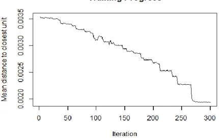
Progression of the Learning Progress. As mentioned above, the plots available in the Kohonen package

are a handy tool to assess the quality of the developed SOM model. Therefore, it makes sense to initiate this evaluation with the assessment of variations along the number of iterations of the model, since it allows us to make some conclusions on the stability of it. The number of iterations is defined in the software routine. However, there should be a certain criterion with the choice of the number of iterations. If the curve that represents the stability of the model is continuously decreasing, more iterations are necessary to consider. In the case of modified credits, 300 iterations were considered, and the Training Progress plot is presented in Figure 5.1.

(28)

20 Figure 5.1 - Training Progress of Modified Credits

Through the analysis of Figure 5.1, it is possible to verify that the number of iterations is sufficient, since as the number of iterations increases, the average distance to the nearest cell in the map decreases, and from nearly 250 iterations we reach stability where there is no longer a continuous decrease of that distance. As such, we can proceed with the model in the way it was defined.

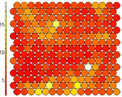
Node Counts Plot. After this first analysis, it is interesting to evaluate the number of instances included

in each neuron, since this allows us to define whether it is necessary to increase or decrease the size of our map. The size of the map must be reduced if there are too many empty cells and increased if there are areas with very high density. This conclusion should be based on the colors of the chart, as we can see in Figure 5.2.

Figure 5.2 - Node Counts of Modified Credits

As mentioned earlier, the distribution should be relatively uniform, which means that, considering the type of graph presented, we should not have large variations in color, i.e., it should be homogeneous. On the left axis of the plot presented in Figure 5.2 we can observe the scale that allows us to interpret this plot. This scale allows us to assess if nodes tend more to the red color, these contain a smaller number of samples, while the lighter color, i.e., if nodes tend more to the yellow color, it means that

(29)

21 these contain a greater number of samples. Evaluating the plot shown in Figure 5.2, we can conclude that there is no major color variation, which makes our distribution relatively uniform, as desired. Additionally, we can notice that there are no empty nodes that would be colored in grey. Additionally, we can observe that there is not a great number of nodes with large values since most contain between 50 and 200 observations. Therefore, there is no need to adjust the size of the map.

Neighbor Distance Plot. As previously mentioned, this plot is often referred to a “U-Matrix”. This

nomenclature because it represents a unified distance matrix. Thus, in this plot, we can visualize a Euclidean distance between the code book vectors of neighboring neurons, represented by colors. As in the graphics presented above, we must guide ourselves by the scale displayed on the left side of the chart.

Figure 5.3 - U-Matrix of Modified Credits

In this type of plot, the rationale we must follow is the intensity of color along with the values presented by the scale. That is, the darker the color, the closer the groups of nodes are, which means that they are more similar. Conversely, neurons with lighter colors represent areas with a greater distance between neurons and, consequently, represent more dissimilar individuals. However, we should not forget to look at the values that the scale presents, since, as we can see in Figure 5.3, we can verify that the distances go from 4 to 16, which means we have neurons relatively close to each other. This plot is particularly important, since the construction of clusters is based on the distance between nodes, considering that each cluster is composed of the nearest neurons.

Clustering. Finally, we have the construction of clusters. The clustering process in the SOM

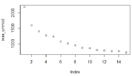
methodology is carried out to group individuals with similar characteristics. This way, it is easier to interpret results and also apply the second methodology of this dissertation, the Markov Chains. However, it is necessary to estimate the optimal number of clusters. For this, an examination of the "within-cluster sum of squares" plot is carried out presented in Figure 5.4.

(30)

22 Figure 5.4 - Optimal Number of Clusters of Modified Credits

The rationale to identify the optimal number of clusters is to find the “elbow point” on the plot, that is, the point at which we verify a slight stabilization of the graphic. Although it is not very obvious, we can see in Figure 5.4 that the elbow point is situated in four clusters, so that is what we must consider. Thus, it is concluded that, in the case of modified credits, we will have four distinct clusters. These clusters can be observed in Figure 5.5.

Figure 5.5 - Clusters of Modified Credits

In Figure 5.5, we can observe the four clusters defined earlier. The green cluster contains nine neurons, the red cluster contains nine neurons, the orange cluster contains 66 neurons, and the blue one contains 15 neurons. Consistently with what was described in the evaluation of the Nodes Count plot, there are no empty nodes, which means that we have observations in all neurons.

Before applying the Markov chain methodology, it is crucial to analyze each cluster in order to be able to characterize them and identify some patterns that may exist within each cluster. This step will be accomplished by analyzing the descriptive statistics of each cluster, and since we have four clusters,