Some issues about the application of the analytic
hierarchy process to R&D project selection
Pedro Godinho*
Fac. Economia, GEMF, Univ Coimbra, Av. Dias da Silva, 165,
3004-512 Coimbra, Portugal E-mail: [email protected] *Corresponding author
João Paulo Costa
Fac. Economia, INESC-C, Univ Coimbra, Av. Dias da Silva, 165,
3004-512 Coimbra, Portugal E-mail: [email protected]
Joana Fialho
Escola Sup. de Tecnologia e Gestão de Viseu, INESC Coimbra, Campus Politécnico de Repeses,
3504-510 Viseu, Portugal E-mail: [email protected]
Ricardo Afonso
PT Inovação, S.A.,Rua Eng Jose Ferreira Pinto Basto, 3810-106 Aveiro, Portugal
E-mail: [email protected]
Abstract: The analytic hierarchy process (AHP) has been used in the process
of selecting research and development (R&D) projects. Such a selection process usually possesses some particular features that require adjustments in the application of the AHP method, such as the existence of a large number of very different alternatives or the integration of qualitative and quantitative criteria. In this paper, we discuss the application of AHP to the selection of a portfolio of R&D projects, and we propose some methods for handling the issues that arise from such an application.
Keywords: research and development; R&D; analytic hierarchy process; AHP;
project evaluation; project selection.
Reference to this paper should be made as follows: Godinho, P., Costa, J.P.,
Fialho, J. and Afonso, R. (2011) ‘Some issues about the application of the analytic hierarchy process to R&D project selection’, Global Business and
Biographical notes: Pedro Godinho is an Assistant Professor at the Faculty of
Economics of the University of Coimbra, which he joined in 1993. He holds a PhD in Management/Systems Sciences in Organisations, a Master in Financial Economics and a degree in Informatics Engineering from the University of Coimbra. He is also a Researcher at GEMF – Group for Monetary and Financial Studies, Coimbra. His research interests include project analysis and evaluation, real options, game theory and project management. He is the author or co-author of several refereed publications in the fields of finance and operations research.
João Paulo Costa is a Full Professor at the Faculty of Economics, University of Coimbra, Portugal. His research interests include decision support systems, information systems, analysis and evaluation of projects and multi criteria decision analysis/making. He holds a PhD in Business Economics from the University of Coimbra. He is also a Researcher at INESCC – Institute of Computer and Systems Engineering, Coimbra. He is author or co-author of more than 100 refereed publications (journals, book chapters and conference proceedings). He was Main Researcher of various funded research projects. Joana Fialho is a PhD student in ‘Management/Decision Aiding Science’, in the School of Economics of the University of Coimbra, Portugal, with a grant from the Portuguese Foundation for Science and Technology (supervisors: Pedro Godinho, João Paulo Costa). She is a Lecturer in Polytechnic Institute of Viseu, Portugal. She is also a Researcher at INESCC – Institute of Computer and Systems Engineering, Coimbra. She holds a degree in Mathematics from the School of Science and Technology of the University of Coimbra (Portugal) and Masters degree in Information Management, from School of Economics of the University of Coimbra, Portugal.
Ricardo Afonso holds a BSc in Statistics and Operations Research (1988), from the Faculty of Sciences of the University of Lisbon. He also holds an MSc in Information Management in the Organisations (1998) from the School of Economics of the University of Coimbra, as well as a Project Management Professional (PMP)® credential (2009) from the Project Management Institute, Inc. He joined Portugal Telecom Inovação (former CET) in 1988, where he is currently Head of the Innovation System and Projects Unit and responsible for implementing the portfolio and project management processes and methodologies in the company.
This paper is a revised and expanded version of a paper entitled ‘Some issues about the application of the analytic hierarchy process to R&D project selection’ presented at Business & Economics Society International (B&ESI) Conference, Athens, Greece, 15–19 July 2010.
1 Introduction
In this paper, we are concerned with the selection of a portfolio of research and development (R&D) projects by a telecommunications company. The company has three levels of decision: the activity, the aggregate and the top management. An activity is a small project that is planned at short-term. An aggregate is a set of connected activities that are directed towards a specific product or service. Apart from the activity and aggregate decision levels, we also consider the top management decision level, which
defines the company policies and the global strategy. Every year, the company selects a portfolio of activities to be pursued, and we developed an approach for supporting the selection of such a portfolio given constraints on the available resources.
One way to select such an R&D project portfolio is to resort to financial theory, which prescribes that the firms’ investment decisions should aim at maximising shareholder wealth. The net present value (NPV) method, recommended by most textbooks, is based on this principle (Brealey et al., 2006).
In the presence of risk, the usual application of the NPV may lead to incorrect results. So, in the last decades, real options analysis (ROA) has been developed as a way of incorporating risk and the managers’ reactions to risky events in the NPV. R&D projects are usually characterised by a large degree of risk, and have been the subject of several applications of ROA (e.g., Childs and Triantis, 1999; Paxson, 2002; Schneider et al., 2008). Many such applications are concerned with pharmaceutical R&D (e.g., Brach and Paxson, 2001; Loch and Bode Greuel, 2001). Other authors apply ROA to telecommunications, or similar sectors: for example, Godinho et al. (2007) develop a real options model for the R&D projects of a telecommunications company, Schwartz and Zozaya Gorostiza (2003) apply ROA to information technology investments, and Lint and Pennings (2001) apply it to R&D at Philips Electronics.
The application of ROA to R&D projects raises several difficulties. The most important of these are, probably, the difficulty of obtaining the relevant data and the presence of a large degree of uncertainty1 associated with R&D. This means that the
representation of the relevant project outcomes will usually have some degree of arbitrariness, one such example being the long term effects of R&D projects. Thus, a real options model may often lead to incorrect decisions. The presence of uncertainty may also lead to different interpretations of the best way to maximise shareholder wealth, with different stakeholders having different perspectives on the path that should be followed.
Many authors have thus chosen to consider multiple criteria in the selection of R&D projects. This way it is possible to consider the quantifiable financial aspects alongside other issues that are harder to quantify, such as the way the project contributes to the company strategy or the way it improves the relations with clients or partners. For example, Farrukh et al. (2000) develop an approach for the valuation of an R&D programme within a manufacturing company in the aerospace industry, taking into account both the cost and some intangible aspects, such as the extension of company knowledge and the potential for partnerships.
The analytic hierarchy process (AHP) (Saaty, 1980) is a multi criteria framework for decision support. The AHP relies on a hierarchic structure to represent the problem, and is based on pairwise comparisons that use a simple scale of intensities of preference. The support that this framework provides to structuring the decision processes, the ease of use, the intuitiveness of the required comparisons, the flexibility and the numerous examples of successful application are some of its main strengths. Several authors have applied the AHP framework to the selection of R&D projects and related areas. Some examples are: Kumar (2004) develops a system for R&D project evaluation based on the AHP; Chiu and Chen (2007) use the AHP to determine the criteria weights for the valuation of intellectual property patents; Shin et al. (2007) use the AHP to evaluate and rank nuclear R&D projects in the Republic of Korea; Chin et al. (2008) integrate evidential reasoning with AHP in a decision support system for new product development projects.
We based our approach for the selection of a portfolio of R&D projects on the AHP framework. We defined two separate hierarchies for the activities and for the aggregates, but in this paper we will focus on the activities. The top level of the hierarchy describes the general goal of the evaluation, and we assumed it to be the maximisation of a global score. In the level immediately below, we included the type of activity. In the meetings with company representatives, we identified the following types:
• Exploratory research: activities that involve exploring and studying new
technologies, in order to identify interesting new paths of research or application. • Experimental development: activities aimed at advancing in a specific research
direction, usually pursuing a defined goal on a particular application. • Product development and support: activities that should lead directly to the
development of a marketable product, or provide support to an existing product. The level below contains the categories of objectives, which we defined as strategic, financial and operational. Below this level, we defined the criteria themselves. Examples of criteria from the strategic category are the contribution to the company image, acquired skills and strategic partnerships. Criteria in the operational category include technological uncertainty and scarcity of required resources. Financial criteria include the NPV directly attributable to the activity (that is, without considering the strategic and option effects, which are indirectly considered through the other criteria) and the possibility of postponement. Both the categories of objectives and the criteria were defined according to the information gathered in meetings with the company’s representatives.
Our AHP based approach allows the calculation of scores for both the activities and the aggregates they belong to. These scores are then used to build a portfolio of activities to be undertaken. Constraints may be imposed on the selection process, defined by the company policy. Such constraints may be defined as minimum and maximum amounts for the usage of resources by activities belonging to a given type or to a given aggregate. The global approach is outlined by Fialho et al. (2008).
In this paper, we focus on some difficulties arising from the application of AHP to the evaluation of R&D projects, and the way we circumvented them. The first issue that we will address is the combination of scores from both intangible and tangible criteria, when a tangible criterion (the NPV) may take negative as well as positive values. In fact, the AHP may handle both types of criteria, but some care must be taken with criteria that may take negative values. The second issue is the comparison of very different projects. The usual application of AHP involves the pairwise comparison of the different alternatives according to the different criteria, but it may be difficult for a decision-maker, coming from a specific department of the company, to compare an activity from her department with one from a different department with which she is not acquainted. The third and last issue is closely related to the previous one. If all pairs of alternatives are to be compared according to each and every criterion, the number of required comparisons will be unmanageably large, given the large number of activity proposals arriving each year at the company. We defined a method to reduce the number of required comparisons and avoid the need to compare very different alternatives.
The paper is structured as follows. Section 2 outlines the AHP framework. Section 3 discusses the integration of tangible and intangible criteria in AHP, in the context of
R&D evaluation. Section 4 presents the procedure for handling numerous alternatives, which also addresses the comparison of alternatives with very different characteristics. Finally, in Section 5 we present some concluding remarks.
2 The AHP
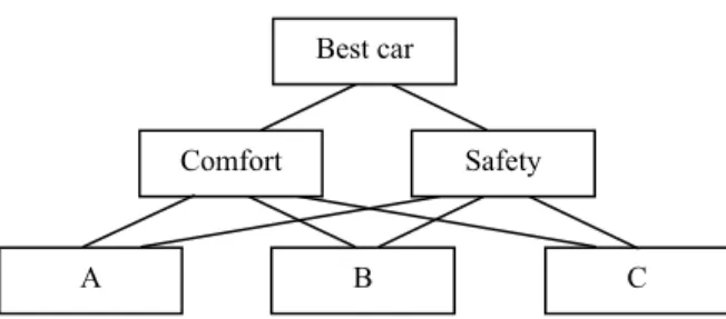
The AHP is a multi criteria framework for decision support that was initially presented in detail in Saaty (1980). The AHP starts by structuring the problem, dividing it into a hierarchy of an overall objective, criteria, subcriteria, sub-subcriteria, etc., with the alternatives placed at the bottom level. To illustrate this, we will consider a simple example concerning the choice of a car. We assume that there are only two relevant criteria: comfort and safety, and we want to choose the best of three alternative cars: A, B and C. Figure 1 illustrates a hierarchy for the problem.
Figure 1 Hierarchy for the choice of a car
The elements at each level of the hierarchy are then pairwise compared according to each element immediately above. In this case, the comfort and safety criteria are compared according to their importance to the ‘Best car’ goal, and the alternatives A, B and C are compared according to both criteria.
Several different scales have been proposed for the pairwise comparisons (Dong et al., 2008), the most usual being the scale proposed by Saaty (1994), which we will use. This scale uses integer numbers from 1 to 9 and their reciprocals. The numbers 1, 3, 5, 7 and 9 correspond to the verbal judgements ‘equal’, ‘moderately more’, ‘strongly more’, ‘very strongly more’ and ‘extremely more’, respectively. The numbers 2, 4, 6 and 8 are used for intermediate levels (e.g., 4 represents ‘moderately to strongly more’), and the reciprocals of the numbers 1–9 are used when the first element is less important than the second (e.g., 1/5 corresponds to ‘strongly less’).
In the example, let us assume that comfort is moderately less important than safety for the overall goal of choosing the best car. Safety will therefore be moderately more important than comfort. A matrix is then built with the values of these pairwise comparisons. For the overall goal, the matrix will be:
Comfort Safety 1 1 Comfort 3 Safety 3 1 ⎡ ⎤ ⎢ ⎥ ⎢ ⎥ ⎣ ⎦ Best car Comfort Safety A B C
The diagonal of each comparison matrix is composed by 1s, since each criteria is equally as important as itself. Since we defined that comfort is moderately less important than safety, we have a12 = 1/3 in the matrix above. Every element aji of the matrix will be the
reciprocal of aij: if a criterion C1 is moderately less important than another criterion C2,
then C2 is moderately more important than C1, so if aij = 1/3 then aji = 3. The same is true
for all the other levels of the scale, so aji = 1/aij.
The elements of the matrix may also be interpreted as the ratio between the weights of the criteria. In the matrix above, since a21 = 3, we will try to assign the safety criterion
a weight three times as large as the weight of the comfort criterion.
In our example, we must also compare the alternatives according to the criteria. We will assume that A is moderately less comfortable than B and weakly more comfortable than C (that is, between equally and moderately more comfortable than C). We also assume than B is strongly more comfortable than C. For the safety criterion, we will assume that A is moderately safer than B and equally safe as C, and that B is strongly less safe than C. So we have the following comparison matrixes:
A B C A B C 1 1 2 1 3 1 A 3 A Comfort : Safety : 1 1 B 3 1 5 B 3 1 5 C 1 1 1 C 1 5 1 2 5 ⎡ ⎤ ⎡ ⎤ ⎢ ⎥ ⎢ ⎥ ⎢ ⎥ ⎢ ⎥ ⎢ ⎥ ⎢ ⎥ ⎢ ⎥ ⎣ ⎦ ⎣ ⎦
From each matrix we derive the priorities of the elements being compared, where the term ‘priorities’ refers to weights, in the case of criteria, or scores, in the case of alternatives. Several different methods have been proposed for the calculation of priorities, but none seems to offer a clear improvement over the original method proposed by Saaty (Dong et al., 2008). According to this method, the priority vector is based on the principal right eigenvector of the comparison matrix (Saaty, 1994). In order to obtain the priority vector, this eigenvector may be normalised in two different ways. The first one corresponds to the most common mode of application of the AHP, the ‘distributive mode’, and consists on normalising the eigenvector so that the sum of the priorities is one. The second one corresponds to the ‘ideal mode’ of the AHP, and consists on normalising the eigenvector so that the largest priority is one.
In our approach for R&D valuation, we use the distributive mode (the most common mode). Using this mode, we get the following priority vectors:
Comfort 0.25 Criteria for best car :
Safety 0.75 ⎡ ⎤ ⎢ ⎥ ⎣ ⎦ A 0.23 A 0.41 Comfort : B 0.65 Safety : B 0.11 C 0.12 C 0.48 ⎡ ⎤ ⎡ ⎤ ⎢ ⎥ ⎢ ⎥ ⎢ ⎥ ⎢ ⎥ ⎢ ⎥ ⎢ ⎥ ⎣ ⎦ ⎣ ⎦
The comparisons introduced by the decision-maker may be subject to some inconsistency due to some possible intransitivity in those comparisons. Saaty (1994) proposes that the inconsistency be measured by a consistency index (CI) defined as
max , 1 λ − = − n CI n
where λmax is the maximum eigenvalue of the comparison matrix and n is the number of
elements being compared. The interpretation of CI depends on the size of the matrix (n). In order to get meaningful values, Saaty (1994) proposes to divide CI by the average consistency index of a matrix of randomly generated comparisons. This average value is termed a random consistency index (RI), and the ratio between CI and RI is termed consistency ratio (CR), and can be interpreted as the percentage of inconsistency in the comparison matrix. Saaty provides the values of RI for several matrix sizes (n × n). Table 1 shows the values of RI for n = 2, ..., 10.
Table 1 Values of the random consistency index (RI) for different matrix sizes (n × n)
n 2 3 4 5 6 7 8 9 10
RI 0 0.52 0.89 1.11 1.25 1.35 1.40 1.45 1.49
Source: Reproduced from Saaty (1994)
From Table 1 we can see that the random comparison matrix of n = 2 has a consistency index of zero. In fact, there can be no inconsistency in a properly built matrix for comparing two elements, since there is only one comparison. This means that CR only becomes meaningful for n ≥ 3. Saaty (1994) suggests thresholds for the acceptable inconsistency of comparison matrixes: a maximum inconsistency of 5% for n = 3, 8% for n = 4 and 10% for n ≥ 5. In our example, the comparison matrix for criteria importance has a null consistency index (since n = 2), and the comparison matrixes for the comfort and safety criteria have CR = 0.36% and CR = 2.79%, respectively. In both cases the value of CR is below the recommended threshold of 5%, so the level of inconsistency present in the matrixes is acceptable.
In order to reach global scores for the alternatives, the priorities thus obtained are multiplied for each path from the hierarchy root to the alternative, and the values corresponding to the same alternative are then added. In our example, this is the same as multiplying the score of each alternative in each criterion by the weight of the criterion. We get the following scores:
0.25 0.23 0.75 0.41 0.365 0.25 0.65 0.75 0.11 0.245 0.25 0.12 0.75 0.48 0.390 = ⋅ + ⋅ = = ⋅ + ⋅ = = ⋅ + ⋅ = A B C s s s
From these scores, we would conclude that the best alternative is car C, closely followed by car A. In this example, the global scores we obtained sum to one – this is always the case when the distributive mode is used. When the ideal mode is used, it is usual to normalise the global scores thus reached, since in this case they do not sum to one.
The AHP is quite flexible, and may be applied in several different ways, for example by rating the alternatives directly instead of comparing them according to the criteria (Saaty, 2006). It has several important benefits, although it also presents some shortcomings, the most well known being rank reversal – the rank of existing alternatives being changed when an irrelevant alternative is added (Belton and Gear, 1983). Saaty (1994, 1997) argues that, if the AHP is properly applied, rank reversal is not a problem.
In the next sections we will present some issues with the application of AHP to the valuation of R&D projects, and explain how we addressed them in our approach.
3 Combining tangible and intangible criteria
Some criteria may have natural numerical values, measured in some predefined unit. Such criteria are termed ‘tangible criteria’. In the example considered in the previous section, this would be the case of the price criterion, if we were to use such a criterion. In fact, price has a natural value, measured in a given currency unit. Such values cannot be directly used in the valuation of alternatives; instead they must be converted to AHP priorities before they are used. In our approach for R&D valuation we consider a single tangible criterion, the NPV, measured in a currency unit (euro).
Saaty (1994) proposes two alternative procedures for the conversion of tangible measures to priorities. The first one consists on converting tangible measures to priorities directly through normalisation; the second one consists on interpreting their relative importance through judgement that is, performing on the tangible criteria the same comparisons that are made on the intangible ones. Saaty recommends the latter procedure as the preferable one.
In the case of the developed approach, neither of these procedures seemed suitable for handling the NPV criterion. In the first one, we would have to assume that the preferences over financial values were linear, which was in discordance with the information gathered in meetings with company representatives. Apart from this problem, we would have to find out a suitable way to handle the normalisation, since NPV may take negative as well as positive values. The second procedure would require the explicit pairwise comparison of the alternatives’ NPVs through the use of the AHP scale. Although such a procedure would be consistent with the way we handle the intangible criteria, it would be unsuitable to the general logic of the approach. The comparisons related to intangible criteria are supposed to require a technical knowledge of the proposed activities, and to be made by aggregate or activity managers, while the preferences over financial values should be determined by the company policy, and therefore be defined by representatives of the company top management. The preferences over financial values should be defined before the activity proposals were made, but it would be impossible to compare the activities’ NPVs before they were known. A possible compromise could be the definition of ranges spanning the possible NPV values, in line with a suggestion made by Saaty (1997). This possibility was also excluded because it could lead to some unsuitable results: if one of the ranges to be used was [5,000 €, 10,000 €[, then a project with an NPV of 5,000 € would have the same score in the NPV criterion as a project with an NPV of 9,999 €, while a project with an NPV of 10,000 € might have a better score than a project with an NPV of 9,999 €, in spite of the differences between NPVs being much smaller in the latter case.
Millet and Schoner (2005) propose a bipolar AHP that can handle criteria whose values may either have a positive or a negative impact on the overall goal, as is the case with the NPV criterion that we are considering. The authors argue that criteria values that provide a negative contribution to the overall goal should be given negative priorities. Their method consists on dividing, for each criterion, the alternatives into two categories: alternatives with a positive contribution to the overall goal and alternatives with a
negative contribution. Alternatives in the same category are compared among themselves, the extreme positive and negative are also compared, and normalisation is performed in a way similar to the ‘ideal mode’. For tangible criteria, the authors present an example concerning the criterion ‘Profit’, which may either take positive or negative values. The authors normalise the criterion values into priorities by assuming that priorities are proportional to the value of the profit – since we do not assume proportional preferences over NPV values, we cannot use this procedure in our approach. However, we could still divide NPV values into positive and negative, and give negative priorities to negative NPVs. In such a case, we would have to follow the bipolar AHP for all the criteria, otherwise we would be handling different criteria inconsistently. But that would make our approach harder to use (the decision-makers would have to divide the set of alternatives into two sets for all criteria whose values might have a positive as well as a negative impact on the overall goal, and compare magnitudes of positive impacts with magnitudes of negative ones). Also, we would introduce additional arbitrariness on the valuation process, through this division between negative and positive impacts. Therefore, we chose not to follow the bipolar AHP.
Since we could not find in the literature a method for handling the NPV criterion suitable to our approach, we developed one. The idea of our method is defining a set of reference values spanning the range of typical NPV values for the activities. The company preferences are defined by comparing the values belonging to this set. Then, we assume that preferences are linear between every consecutive values belonging to this set. This assumption enables us to compare the NPV of any one activity to the values belonging to this set. This way, we are able to automatically build an extended comparison matrix containing the reference values as well as the activities’ NPVs. We calculate the priorities given by this extended matrix, remove from the priority vector the priorities of the reference values and normalise the priorities of the alternatives. This way, we get a vector of priorities that can be used identically to the ones obtained for the other criteria. We will now present an example that illustrates this method.
For the sake of simplicity, let us consider just three reference values of –100, 0 and +100, and two activities with NPVs of –25 and +50. Before the activities are proposed, the representatives of top management define the comparisons between the reference values. Let us assume that the following comparison matrix was obtained for the reference values: 100 0 100 1 1 1 3 6 100 1 0 3 1 2 100 6 2 1 − + ⎡ ⎤ − ⎢ ⎥ ⎢ ⎥ ⎢ ⎥ + ⎢ ⎥ ⎢ ⎥ ⎣ ⎦
From this matrix, we would get the priorities p–100 = 0.10, p0 = 0.30 and p100 = 0.60 for
the values –100, 0 and +100, respectively. –25 is between –100 and 0, and we can write –25 = –100 + 0.75 (0 – (–100)). So, given the priorities of the reference values and assuming linear preferences between –100 and 0, the priority of –25, p–25, can be
calculated as:
(
)
(
)
25 100 0.75 0 100 0.10 0.75 0.30 0.10 0.25
− = − + ⋅ − − = + ⋅ − =
The comparisons between –25 and the reference values are defined by the ratios between their priorities. That is, the pairwise comparison between –100 and –25 will lead to a relative value of p–100 / p–25 = 0.10 / 0.25 = 0.40.
The value of 0.40 does not belong to the comparison scale defined in Section 2, but this is not a problem. According to Saaty (1997), the scale is only intended as a convenient support for pairwise judgements made by human decision-makers and, if that is useful, values outside the scale can be used in the comparisons.
The relative values of the other comparisons could be obtained in a similar way. Similarly, for the NPV of +50, we get a priority of 0.45, and may then define the relative values of the comparisons. This way, we get the extended matrix:
100 0 100 25 50 0.1 0.1 1 1 1 100 3 6 0.25 0.45 0.3 0.3 1 3 1 0 2 0.25 0.45 0.6 0.6 6 2 1 100 0.25 0.45 0.25 0.25 0.25 1 25 0.1 0.3 0.6 0.45 0.45 0.45 1 50 0.1 0.3 0.6 − + − + ⎡ ⎤ − ⎢ ⎥ ⎢ ⎥ ⎢ ⎥ ⎢ ⎥ + ⎢ ⎥ ⎢ − ⎥ − ⎢ ⎥ ⎢ − ⎥ + ⎢⎣ ⎥⎦
Notice that the extended comparison matrix is not complete: the pairwise comparisons between the activities’ NPVs are not introduced. We use a method proposed by Harker (1987) that allows us to calculate priorities from an incomplete matrix as long as all the elements are compared either directly or indirectly. In matrixes such as the above, this condition always holds: only the direct comparisons between activities’ NPVs are missing, but indirect comparisons, defined through the comparisons between activities’ NPVs and reference values, are always present. In the example, only the direct comparison between –25 and +50 is missing, but both these values are directly compared to the reference values, thus defining an indirect comparison between the two of them.
The matrix presented before leads to a vector of priorities:
[
0.059 0.176 0.353 0.147 0.265]
TSince we are only interested in the priorities of the activities’ NPVs, we only consider the last two elements of the vector, and normalise them so that they sum to one. We thus get priorities of 0.357 and 0.643 for the NPVs of –25 and +50, respectively. These priorities can be combined with the priorities derived for intangible criteria when using the distributive mode of the AHP, as we do in our approach.
In the meetings with company representatives, we were able to conclude that preferences over positive NPVs could be assumed to be linear, although the same assumption does not hold for negative NPVs. This information enabled us to simplify the process of eliciting the company preferences over NPVs. It is enough to define a set of reference values that includes a zero value as well as additional values spanning the range of typical negative NPVs. The pairwise comparisons between these reference values, along with the assumption of linearity for positive values, allow us to compare any positive or negative NPV with the reference values. This way we are able to build the extended matrix, and calculate the priorities of the activities’ NPVs.
4 Handling a large number of alternatives
Two potential difficulties with the application of AHP are related to the need of performing a large number of comparisons, and comparing very different alternatives (Saaty, 1994, 1997). In fact, Saaty (1994) recommends that comparisons should involve sets of no more than seven elements. In the case of the company we are considering, these were important issues, since every year it is necessary to choose from a large set of activity proposals, with very different alternatives coming from various departments of the company. Comparing all pairs of proposals according to all the criteria would thus be unmanageable.
Triantaphyllou (1999) suggests a duality procedure for reducing the number of required comparisons. Within this procedure, the typical questions made to the decision-maker require her to compare the importance of two criteria in terms of an alternative, instead of comparing two alternatives according to a criterion (as usual in AHP). This procedure reduces the number of required comparisons whenever the number of alternatives is larger than the number of criteria plus one. In the case of our approach, although this procedure would reduce the number of required judgements, it would still require an unmanageably large number of comparisons, since the number of relevant criteria are quite large (six strategic, four operational and five financial criteria). Also, the type of comparisons required by the duality procedure was judged to be less intuitive than the usual AHP comparisons, so we did not incorporate this procedure in our approach.
Islam and Abdullah (2006) propose a technique for excluding criteria that carry a small weight, and suggest this as a way of reducing the number of required comparisons. Since the criteria that we identified in meetings with the company representatives were considered important, their exclusion might make it more difficult for the approach to be well accepted in the company – in fact, all the irrelevant criteria were excluded before we settled on the final set. Apart from that, the exclusion of some criteria would still lead to an unmanageably large number of required comparisons, and would not address the problem of comparing very different alternatives.
A usual way of addressing the problem of having a large number of possibly very different alternatives is through the clustering of alternatives. Saaty (1997) describes a method based on the construction of clusters of homogeneous alternatives. After the clusters are built, they are ordered based on the similarity of the alternatives. The alternatives within the first cluster are then compared among themselves, and their priorities are calculated. The alternative belonging to the first cluster that is most similar to the ones belonging to the second one is then placed on the second cluster and the priorities of this ‘extended’ second cluster are determined. Then, an alternative from the second cluster is placed on the third one, and the process goes on until the priorities are calculated for all the clusters. The common element of each two consecutive clusters allows the calculation of priorities that are consistent across the different clusters – for example, if the common alternative of the first and second clusters has a priority of 0.20 in the first one and a priority of 0.05 in the second one, then by dividing all the priorities obtained in the first cluster by four we get a set of priorities that is consistent with the priorities derived for the second one. So, with this method we get a set of priorities for all the elements, without having either to compare very large sets of alternatives, or very disparate ones. Triantaphyllou (1995) proposes a linear programming based procedure for combining the comparisons of two matrixes with common elements in order to derive the priorities of the elements of both matrixes. Such a procedure allows the extension of
Saaty’s clustering method by considering the construction of ‘extended’ clusters with more than one common element. The method for handling incomplete matrixes proposed by Harker (1987) (considered in Section 3) allows the construction of an extended incomplete matrix by joining the comparisons of any number of matrixes with common elements. This way, Harker’s method also allows an extension of the method described by Saaty.
Hotman (2005) proposes a base reference AHP that allows the reduction of the number of comparisons. The method starts by defining a base alternative, and all the other alternatives are only compared to this base alternative. From these comparisons the calculation of priorities can be performed in quite a simple way. In fact, in spite of reducing the number of required comparisons, this method does not address the need of comparing very different alternatives.
Our approach uses some ideas from both the clustering method and the base reference AHP. Instead of defining just one reference activity, we define a set of artificial reference activities, or benchmark activities, which is wide enough to span the range of types of alternatives typically proposed in each year. The alternatives belonging to this set are compared among themselves. These comparisons are considered to reflect the company policies, so they are performed by representatives of the company management before the activity proposals are evaluated. The method for handling incomplete matrixes proposed by Harker (1987) is used for reducing the number of required comparisons. If there are n reference activities, then only n – 1 comparisons are required to completely define the relations between all the activities according to an intangible criterion [instead of the (n – 1) ⋅ (n – 2) / 2 required to directly compare all the pairs of alternatives].
Consider a small example, where there are only three reference activities, R1, R2 and
R3. If, for a given criterion, R1 and R3 are too disparate, then we would only compare R1
to R2 and R2 to R3. These two comparisons would indirectly relate R1 to R3. For
illustration purposes, we will consider that, according to a given criterion C, R1 is
moderately preferred to R2 and R2 is strongly preferred to R3. We would get the following
incomplete comparison matrix:
1 2 3 1 2 3 R R R 1 3 R 1 R 3 1 5 R 1 1 5 ⎡ −⎤ ⎢ ⎥ ⎢ ⎥ ⎢ ⎥ ⎢− ⎥ ⎢ ⎥ ⎣ ⎦
After the reference activities are compared according to all the criteria, the proposed activities (that is, the ones we really want to assess) can be evaluated.
We consider two alternative procedures for eliciting the comparisons concerning the proposed activities. The first one consists on building matrixes that include one proposed activity and the reference activities. In this case, for a given proposed activity and for a given criterion, it is enough to compare it with the most similar reference activity. Since we are using Harker’s method and the reference activities are compared among themselves, the comparison with a single reference activity suffices to indirectly relate the proposed activity to all the other reference activities.
Let us assume, for illustration purposes, that there are only two proposed activities, A and B, and one criterion C. A is closely related to R1, and can be considered as good as
R1 according to this criterion. B is closely related to R3, and can be considered slightly
better than R3 according to criterion C. These two comparisons would suffice to evaluate
both activities according to criterion C; however, if the decision-maker considered it preferable, she might also include other comparisons, in order to express her preferences in more detail.
Considering only the mentioned comparisons, we would get the following matrixes:
1 2 3 1 2 3 1 1 2 2 3 3 R R R A R R R B 1 3 1 1 3 R R 1 1 5 1 1 5 R 3 R 3 R 1 1 R 1 1 1 5 5 2 A 1 1 B 2 1 − − − ⎡ ⎤ ⎡ ⎤ ⎢ ⎥ ⎢ ⎥ − − ⎢ ⎥ ⎢ ⎥ ⎢ ⎥ ⎢ ⎥ − − − ⎢ ⎥ ⎢ ⎥ ⎢ ⎥ ⎢ ⎥ − − − − ⎢ ⎥ ⎢ ⎥ ⎣ ⎦ ⎣ ⎦
The method for incomplete matrixes proposed by Harker (1987) allows us to derive priorities from each of these matrixes. Similar matrixes would be obtained for all criteria, and a global score would be calculated for each of the proposed activities. Since all the scores are related to the comparison with the same reference alternatives, they can be compared and used to rank the proposed activities.
In the example, let us assume that C is the only criterion. The priorities according to this criterion will therefore be equal to the global score. By using the matrixes presented before, we get a score of 0.417 for A and 0.087 for B, leading us to conclude that A is preferable to B (notice that we also get scores for the reference activities, but since we want to compare A to B, these scores will not be relevant). The activities’ scores can be normalised to 0.83 and 0.17 for A and B, respectively.
The second way of eliciting comparisons consists on letting the decision-maker enter the comparisons into a matrix containing both the reference and the proposed activities. The comparisons must allow all activities to be directly or indirectly related, but now a proposed activity can be compared to another proposed activity instead of a reference one (as long as the latter proposed activity is directly or indirectly related to a reference activity).
Returning to the example that we have been following, and assuming once again the same comparisons, we would get the following matrix:
1 2 3 1 2 3 R R R A B R 1 3 1 1 R 3 1 5 1 R 5 1 0.5 A 1 1 B 2 1 − − ⎡ ⎤ ⎢ ⎥ ⎢ − − ⎥ ⎢ ⎥ ⎢− − ⎥ ⎢ ⎥ ⎢ − − − ⎥ ⎢ ⎥ ⎢− − − ⎥ ⎣ ⎦
This matrix allows us to get the scores 0.395 and 0.053 for A and B, respectively. Therefore the rank of the proposed alternatives is the same as before. These scores can be normalised to 0.88 and 0.12 for A and B, respectively.
The use of any of these procedures allows the number of required comparisons to be reduced to a manageable level (one comparison for each proposed activity and each intangible criterion). The use of reference activities also circumvents the problem of comparing very different activities, and introduces the company policy in the valuation process through the definition of benchmarks. Finally notice that, for the NPV, no comparisons are required when the proposed activities are being evaluated: each proposed activity will have an NPV, and an NPV will also be defined for each of the reference activities. This way, the method described in Section 3 can be applied to automate the calculation of priorities for the NPV criterion.
5 Final remarks
In this paper we considered an approach for the selection of an R&D portfolio based on the AHP. We considered some important issues with the application of AHP to the selection of such a portfolio, namely the need to combine the tangible NPV criterion with other intangible criteria, and the necessity of handling a large number of alternatives, some of them possibly very different and therefore difficult to compare.
We proposed a method for deriving priorities from the NPV values, based on a set of comparisons of predefined reference values that reflect the company preferences. Once those comparisons are defined, the proposed method allows the priorities to be obtained automatically from the NPV values.
The method for handling a large number of possibly very different alternatives involves the definition of reference alternatives that should span the types of alternatives usually considered in the selection process. The use of those reference alternatives, along with a method that allows priorities to be derived from incomplete matrixes, allows us to achieve global scores from a manageable number of comparisons, and to ensure that there is no need to compare very disparate alternatives.
The tests made on this approach for selecting an R&D portfolio showed it to be effective. So, the solutions proposed for the problems addressed in this paper seem to work very well, and they had a good acceptance in the considered telecommunications company.
Acknowledgements
This research was supported by Portugal Telecom Inovação. J. Fialho was supported by FCT under grant SFRH/BD/41157/2007.
References
Belton, V. and Gear, T. (1983) ‘On a shortcoming of Saaty’s method of analytic hierarchies’,
Omega, Vol. 11, No. 3, pp.228–230.
Brach, M. and Paxson, D. (2001) ‘A gene to drug venture: Poisson options analysis’, R&D
Management, Vol. 31, No. 2, pp.203–214.
Brealey, R., Myers, S. and Allen, F. (2006) Principles of Corporate Finance, 8th ed., Irwin/McGraw-Hill.
Childs, P.J. and Triantis, A.J. (1999) ‘Dynamic R&D investment policies’, Management Science, Vol. 45, No. 10, pp. 1359 1377.
Chin, K.S., Xu, D., Yang, J.B. and Lam, J. (2008) ‘Group-based ER-AHP system for product project screening’, Expert Systems with Applications, Vol. 35, No. 4, pp.1909–1929.
Chiu, Y.J. and Chen, Y-W. (2007) ‘Using AHP in patent valuation’, Mathematical and Computer
Modelling, Vol. 46, Nos. 7–8, pp.1054–1062.
Dong, Y., Xu, Y., Li, H. and Dai, H. (2008) ‘A comparative study of the numerical scales and the prioritization methods in AHP’, European Journal of Operational Research, Vol. 186, No. 1, pp.229–242.
Farrukh, C., Phaal, R., Probert, D., Gregory, M. and Wright, J. (2000) ‘Developing a process for the relative valuation of R&D programmes’, R&D Management, Vol. 30, No. 1, pp.43–53. Fialho, J., Godinho, P., Costa, J.P., Afonso, R. and Regalado, J.G. (2008) ‘A level based approach
to prioritize telecommunications R&D’, Journal of Telecommunications and Information
Technology, No. 4, pp.40–46.
Godinho, P., Regalado, J.G. and Afonso, R. (2007) ‘A model for the application of real options analysis to R&D projects in the telecommunications sector’, Global Business and Economics
Anthology, II, December, pp.414–422.
Harker, P. (1987) ‘Incomplete pairwise comparisons in the analytic hierarchy process’,
Mathematical Modelling, Vol. 9, No. 11, pp.837–848.
Hotman, E. (2005) ‘Base reference analytical hierarchy process for engineering process selection’, in Khosla, R., Howlett, R. and Jain, L. (Eds.): Knowledge Based Intelligent Information and
Engineering Systems, Part 1, pp.184–190, Springer Verlag.
Islam, R. and Abdullah, N. (2006) ‘Management decision making by the analytic hierarchy process: a proposed modification for large scale problems’, Journal of International Business
and Entrepeneurship Development, Vol. 3, Nos. 1/2, pp.18–40.
Knight, F. (1921) Risk, Uncertainty and Profit, Houghton Mifflin Company, Chicago
Kumar, S.S. (2004) ‘AHP based formal system for R&D project evaluation’, Journal of Scientific
and Industrial Research, Vol. 63, No. 11, pp.888–896.
Lint, O. and Pennings, E. (2001) ‘An option approach to the new product development process: a case study at Philips Electronics’, R&D Management, Vol. 31, No. 2, pp.163–172.
Loch, C.H. and Bode Greuel, K. (2001) ‘Evaluating growth options as sources of value for pharmaceutical research projects’, R&D Management, Vol. 31, No. 2, pp.231–248.
Millet, I. and Schoner, B. (2005) ‘Incorporating negative values into the analytic hierarchy process’, Computers & Operations Research, Vol. 32, No. 12, pp.3163–3173.
Paxson, D. (Ed.) (2002) Real R & D Options, Butterworth Heinemann. Saaty, T.L. (1980) The Analytic Hierarchy Process, McGraw Hill, New York.
Saaty, T.L. (1994) Fundamentals of Decision Making and Priority Theory with the Analytic
Hierarchy Process, RWS Publications.
Saaty, T.L. (1997) ‘That is not the analytic hierarchy process: what the ahp is and what it is not’,
Journal of Multi Criteria Decision Analysis, Vol. 6, No. 6, pp.320–339.
Saaty, T.L. (2006) ‘Rank from comparisons and from ratings in the analytic hierarchy/network processes’, European Journal of Operational Research, Vol. 168, No. 2, pp.557–570.
Schneider, M., Tejeda, M., Dondi, G., Herzog, F., Keel, S. and Geering, H. (2008) ‘Making real options work for practitioners: a generic model for valuing R&D projects’, R&D Management, Vol. 38, No. 1, pp.85–106.
Schwartz, E.S. and Zozaya Gorostiza, C. (2003) ‘Investment under uncertainty in information technology: acquisition and development projects’, Management Science, Vol. 49, No. 1, pp.57–70.
Shin, C.O., Yoo, S-H. and Kwak, S-J. (2007) ‘Applying the analytic hierarchy process to evaluation of the national nuclear R&D projects: the case of Korea’, Progress in Nuclear
Triantaphyllou, E. (1995) ‘Linear programming based decomposition approach in evaluating priorities from pairwise comparisons and error analysis’, Journal of Optimization Theory and
Applications, Vol. 84, No.1, pp.207–234.
Triantaphyllou, E. (1999) ‘Reduction of pairwise comparisons in decision making via a duality approach’, Journal of Multi Criteria Decision Analysis, Vol. 8, No. 6, pp.299–310.
Notes
1 We use the classical distinction between risk and uncertainty, according to which risk is susceptible of measurement and uncertainty is not (Knight, 1921).