Copyright © 2016 Techno-Press, Ltd.
http://www.techno-press.com/journals/eas&subpage=7 ISSN: 2092-7614 (Print), 2092-7622 (Online)
Development of fragility curves for RC bridges subjected to
reverse and strike-slip seismic sources
Araliya Mosleh
1, Mehran S. Razzaghi
2, José Jara
3and Humberto Varum
41Department of Civil Engineering, Faculty of Engineering, University of Aveiro, 3810-193 Aveiro, Portugal 2Department of Civil Engineering, Qazvin Branch, Islamic Azad University, Qazvin, Iran
3Department of Civil Engineering, Faculty of Engineering, Universidad Michoacana de San Nicolas de
Hidalgo, Morelia, Mexico
4CONSTRUCT-LESE, Department of Civil Engineering, Faculty of Engineering, University of Porto,
4200-465 Porto, Portugal
(Received May 6, 2016, Revised September 5, 2016, Accepted September 6, 2016)
Abstract. This paper presents a probabilistic fragility analysis for two groups of bridges: simply supported and integral bridges. Comparisons are based on the seismic fragility of the bridges subjected to accelerograms of two seismic sources. Three-dimensional finite-element models of the bridges were created for each set of bridge samples, considering the nonlinear behaviour of critical bridge components. When the seismic hazard in the site is controlled by a few seismic sources, it is important to quantify separately the contribution of each fault to the structure vulnerability. In this study, seismic records come from earthquakes that originated in strike-slip and reverse faulting mechanisms. The influence of the earthquake mechanism on the seismic vulnerability of the bridges was analysed by considering the displacement ductility of the piers. An in-depth parametric study was conducted to evaluate the sensitivity of the bridges’ seismic responses to variations of structural parameters. The analysis showed that uncertainties related to the presence of lap splices in columns and superstructure type in terms of integral or simply supported spans should be considered in the fragility analysis of the bridge system. Finally, the fragility curves determine the conditional probabilities that a specific structural demand will reach or exceed the structural capacity by considering peak ground acceleration (PGA) and acceleration spectrum intensity (ASI). The results also show that the simply supported bridges perform consistently better from a seismic perspective than integral bridges and focal mechanism of the earthquakes plays an important role in the seismic fragility analysis of highway bridges.
Keywords: fragility curves; seismic vulnerability; simply supported bridges; integral bridges; reverse and strike-slip seismic sources
1. Introduction
Past earthquakes that have occurred in seismically active areas, show that bridge structures are one of the most vulnerable and expensive components of highway transportation systems. Bridge
service interruptions may lead to loss of lives and/or economic losses during or after an earthquake event (Sheikh and Tsang 2011, Venkittaraman 2013, Wang et al. 2013). During the past decades, several bridges have been damaged due to the occurrence of earthquakes or other natural disaster (Eshghi and Razzaghi 2004, Nicknam et al. 2011, Wang et al. 2009, Wang and Lee 2009, Lin et
al. 2015). Hence, the study of the expected seismic performance of bridges has attracted the
attention of several researchers and research groups during the last decades (Jara et al. 2013a, Jara
et al. 2013b, Varum et al. 2011, Zhang et al. 2008, Lin et al. 2015). The seismic vulnerability of
highway bridges is usually expressed in the form of fragility curves developed through probabilistic analysis (ATC 1985, Gehl and Ayala 2016, Jeon et al. 2015, Padgett and DesRoches 2008, Shinozuka et al. 2000). Fragility curves for class of bridges present the relationship between the probability of reaching or exceeding a certain damage state as a function of ground motion intensities (ATC 1985, Billah and Alam 2015). Fragility curves are useful for structures located on low and high seismic regions in order to develop retrofit programs, conduct pre-earthquake planning and post-earthquake response and evaluation. Several methodologies are developed to generate bridge fragility curves. One approach utilizes expert opinions due to earthquake damage and loss estimates to generate fragility curves for transportation facilities, including bridges (Rossetto and Elnashai 2003). Another way to develop fragility curves is the use of damage distribution functions determined based on post-earthquakes field observations or reconnaissance reports. Several other researchers developed empirical fragility curves based on the post-earthquake damage data and observations (Der Kiureghian 2002, Elnashai et al. 2004, Yazgan 2015). Basoz and Kiremidjian (Basoz and Kiremidjian 1997) present a logistic regression analysis to generate empirical fragility curves for the Northridge earthquake bridges damaged data, while Shinozuka et al. (Shinozuka et al. 2001) used the parameters of a lognormal probability distribution estimated by the Maximum Likelihood Method for Kobe earthquake data. In the lack of adequate damage data or expert option, analytical fragility curves are the best choice to assess the seismic performance of highway bridges. The curves can be developed by a variety of analytical methods, such as elastic spectral method (Hwang 2000), nonlinear static analysis (Dutta and Mander 1998, Loh et al. 2002, Monti and Nistico 2002, Banerjee and Shinozuka 2007, Siqueiraa et al. 2014), nonlinear response history analysis (NLTHA) (Hwang et al. 2001, Karim and Yamazaki 2003, Choi et al. 2004, Elnashai et al. 2004, Choine et al. 2015, Ramanathana et al. 2015, Yang et al. 2015, Mosleh et al. 2016a, Nateghi and Shahsavar 2004) and incremental dynamic analysis (IDA) (Billah et al. 2013, Billah and Alam 2016, Dezfuli and Alam 2016). In the past decades, there have been significant researches regarding seismic vulnerability of buildings, however, less investigation has been devoted to bridges (Bojórquez et al. 2012, Mollaioli et al. 2013, Mosleh et al. 2016b). Also, a large number of highway bridges around the world do not achieve the seismic detailing requirements recommended in current codes and guidelines (Caltrans 2013). Therefore, the development of fragility functions, particularly in what concerns some particular classes of bridges, should be a high priority in research activities.
In the past decades, the construction of integral and continuous bridges in recent decades is growing, the implementation of these bridges in some countries is limited due to technical issues and existing regulations (Denton and Tsionis 2012). One of the most important advantages of integral bridges is the elimination of expansion joints, which reduces maintenance costs during the structure life. The installation and maintenance of the expansion joints are expensive and sometimes the replacement is even more costly. Another advantage of integral bridges is the avoidance of corrosion problems, which are frequently present in expansion joints and seals that permit salt-laden run-off water from the roadway surface to make contact with the substructure
elements. Many problems may originate from leaky joints (Mistry 2005). In addition, elastomeric glands can be filled up by trash, clods, and little stones and fail to function properly. Furthermore, steel bearings can be exposed to corrosion and elastomers can split or rupture due to sudden and unpredictable movements (Paraschos and Amde 2011). Hence, integral bridge construction provides better durability performance and lower bridge operating costs. Moreover, the reduction of joints in bridge structures leads to substantial savings in the costs of construction and maintenance. In particular, the number of bearings in each pier is substantially reduced when compared with the case of simply supported multiple-span decks. Another advantage of integral bridges is the elimination of the unseating superstructure problem. Moreover, the moment-resisting connection between superstructure and substructure offers enhanced redundancy in the bridge and the energy dissipation capability is increased by increasing the number of plastic hinges required to form a collapse mechanism. However, it should be noted that greater demands may be transferred from superstructure to substructure in integral systems (Frosch et al. 2009). Previous researchers provide different approaches to evaluate the seismic performance of bridges with different types of superstructures (Choi et al. 2004, Avsar et al. 2011). Only a few studies have been carried out to compare the seismic performance of simply supported bridges with integral structures subjected to different seismic sources (Nielson and DesRoches 2007a, Choine et al. 2015).
In this study, analytical fragility curves for two common classes of bridges are developed. Comparisons considering seismic fragility based on different seismic sources are also drawn. First of all, an outline of the used methodology is explained. Secondly, the classification of bridges, ground motion selection, definition of damage states, real construction practices, and results of the nonlinear dynamic analyses are presented. Thirdly, the fragility curves used to assess the seismic vulnerability of common bridges by considering different intensity measures are described. Finally, the fragility curves associated with reverse and strike-slip seismic sources are compared.
2. Bridge characteristics
This study develops fragility curves for two bridge classes subjected to ground motions of two seismic sources. For both the simply supported and integral bridge classes, a group of concrete bridges in Iran are modelled. Two major bridge classes are analysed: simply supported structures on elastomeric bearings at the seat abutments and column bents and continuous bridges. Based on
Table 1 Structural attributes for the bridge samples for each two bridge classes Bridge classes Column height (Hcol) , (m) Column Diameter (m) Longitudinal steel ratio (%) Span length (L) , (m) Number of spans 1st natural period (s) Bearing stiffness (kN/mm) Column Abutment Kz Kv Kz Kv CC-C 4 1.0 1.125 20 4 0.36 - - 1077 3.12 CC-C 6 1.0 1.125 20 4 0.63 - - 1077 3.12 CC-C 8 1.0 1.125 20 4 0.73 - - 1077 3.12 CC-S 6 1.1 1.2 24 4 0.99 695 2.53 695 2.53 CC-S 9 1.2 1.56 32 6 1.38 5024 5.63 13219 10.8 CC-S 10.5 1.3 1.06 20 6 1.17 5023 5.59 13214 10.79
the superstructure connection, section bridge classes are divided into column-continuous (CC-C) and column-simply supported (CC-S) bridges. Fig. 1 displays schematic drawings of sample bridges in the longitudinal and transverse directions and their components that constitute the general attributes of the bridges. The models include different bridge lengths and column heights. Table 1 shows the overall dimensions of the bridges and structural attributes of the bridge samples for each two bridge class. Circular solid columns are considered for two major bridge classes. Based on the analysis of Iran bridge inventory, Mosleh (Mosleh 2016) found that most of the bridges in Iran have skew angles less than 5°, therefore the effect of skew angle is eliminated in this study (Mosleh et al. 2016a).
For each bridge class, different case studies are considered; Shinozuka et al. (Shinozuka et al. 2000) considered ten sample bridge classes, whereas six samples were analyzed by Choine et al. (Choine et al. 2015). Nielson (Nielson 2005) considered eight sample case studies for each bridge classification. In this study, for each bridge classification, three real bridges are considered as case studies.
3. Numerical analysis of the bridges
Nonlinear response history analyses are accomplished by adopting a three-dimensional structural model (Fig. 2), using SAP 2000 (Computers and Structures Inc. 2009) software. The superstructure is composed of cast-in-place reinforced concrete (RC) slabs over RC girders in the CC-S system and voided slabs supported on columns in CC-C structures. Voided slabs were introduced in the software by considering the equivalent moment of inertia and a mass correction factor. The superstructure mass includes slabs, girders, diaphragms, parapets, asphalt, and sidewalks. Superstructure elements are assumed to remain in the elastic range of behaviour and are protected by a capacity design for simply supported bridges. However, for integral bridges, the bending moment demands in deck in all analyses were determined and verified that demands are in the range of the elastic behaviour in the slab. This bridge behaviour is understandable considering the limited quantities of longitudinal reinforcement in piers of old Iran bridges that make the columns weak elements. Shell elements are utilized to model the deck and diaphragms. The substructure of the bridge consists of the bent system and abutments. Elastomeric bearings, modelled using link elements, are located between the substructure and superstructure. Frame elements are utilized to model the columns, girders, and the cap beams by considering six degree of freedom at each node. By taking into account the Caltrans recommendation (Caltrans 2013), elastic springs in the longitudinal and transverse directions are utilized to model the abutments and backfill soil. The abutments are designed to provide unimpeded traffic access from the bridge and an economical means of resisting bridge inertial loads developed during ground excitations. The resisting movement at the abutment is provided by backfill passive pressure force, and it depends on the material properties of the backfill. Abutment longitudinal response analysis could be explained by utilizing a bilinear approximation of the force-deformation relationship or the nonlinear force-deformation relationship (Shamsabadi 2007).
The bilinear demand, which includes the effective abutment stiffness, is influenced by expansion gaps, and it includes a realistic value for the embankment fill response. Based on force deflection results from large-scale abutment testing (Maroney 1995, Shamsabadi 2007, Stewart et
al. 2007) and passive earth pressure, the initial stiffness Ki is considered as14.35 kN/mm/m
be adjusted proportionally to the back-wall height of the abutment as: Kabut=Ki×wa×(ha/1.7), where
ha and wa are the height and width of the back-wall for seat abutments, respectively.
Soil-structure interaction is neglected assuming hard soil sites and column bents are fixed at the bottom. Elastomeric bearings are located between the superstructure and substructure components, without any dowel or connecting device. The lateral and vertical stiffnesses of the elastomeric bearing were modelled as a spring, as proposed by Priestly et al. (Priestly et al. 1996).
Shear bearing stiffness can be calculated as Kv=
h GA
, where G is the shear modulus of rubber (taken as 1 MPa), A is the gross rubber area, and h is the total rubber height. Vertical bearing
(a) (c)
(b) (d)
Fig. 1 General characteristics of (a) simply supported bridge, (b) integral bridge, (c) transverse view of simply supported bridge and (d) transverse view of integral bridge
stiffness is determined as Kz= h K GS GAKS ) (6 6 2 2
, where k is the rubber bulk modulus and S is the shape
factor (Table 1). The mass and stiffness proportional Rayleigh damping coefficients were determined considering the first two modal periods (Aviram et al. 2008). Nonlinear analyses with direct integration, including P-∆ effects, were conducted in two orthogonal directions to evaluate the seismic vulnerability of the bridges.
To determine the material properties of the bridge elements, concrete cores and bars specimens were obtained (Fig. 3). Three samples of each bridge component were collected. Table 2 shows mean values of specimen strengths obtained after testing in laboratory. The longitudinal reinforcement was tested in tension to determine the class of reinforcing steel, yield stress, and ultimate stress. The concrete strength was also determined by conducting test with a Schmidt hammer.
It is important to remark that nonlinear behaviour of the structure is obtained directly from the nonlinear stress-strain relationship of concrete and steel, therefore the reliability of nonlinear bridge members depends on the accuracy of the material properties considered. Reinforcing steel bars are modelled utilizing bilinear steel material model with kinematic hardening behaviour
according to the Caltrans recommendation (Caltrans 2013). Nominal yield strain (ɛy) and expected
yield strain (ɛye) are considered as 0.0021 and 0.0023, respectively, the ultimate tensile strain (ɛsu)
that is bar size dependent is determined as 0.12. The effect of confinement is to enhance the compression strength and ductility capacity on concrete. For the confined concrete, previous researchers developed different stress-strain relationships (Bazant and Bhat 1976, Kent and Park 1971, Mander et al. 1988, sheikh and Uzumeri 1980). Some of the proposed methods have restriction in the range of condition (e.g., circular or rectangular sections), however the method suggested by Mander et al. (Mander et al. 1988) is applicable to all section shapes and all levels of confinement according to the following equations
1.254) 2 7.94 1 (2.254 ' c ' l ' c ' l ' c ' cc f f f f f f (1) 1) 5 0.002(1 ' c ' cc cc f f ε (2) ' cc su yh s cu f ε f ρ ε 0.0041.4 (3) yh s e ' l h s f k ρ f s D' A ρ 2 1 4 (4)
where f´cc and ɛcc are concrete stress and strain at peak stress, f´l is the effective lateral confining
stress and ɛcu is the ultimate compression strain respectively. fyh is the yield strength of the
transverse reinforcement, εsu is the steel strain at the maximum tensile stress, f′cc is the compressive
strength of the confined concrete, ρs is the volumetric ratio of confining steel, Ah is the
cross-sectional area of transverse reinforcement, D′ is the diameter of the confined concrete core, ke is
confinement coefficient, ρcc is the ratio of area of longitudinal reinforcement to area of core of the
(a) (b) (c)
Fig. 3 Characterization procedures and sampling (a) soil around the abutment to obtain the abutment dimension, (b) longitudinal and transversal reinforcements, (c) Facial reconstruction after the procedures Table 2 Statistical material properties of highway bridges in Iran
f´c (col) MPa f´c (cap beam) MPa f´c (girder) MPa fsy (bar) MPa fsu(bar) MPa CC-C 31 - - 392 588 CC-S 24 24 16-27 392-520 588-665
elasticity (Ec) for normal weight concrete and Shear modulus, Gc, for ν=0.2 are determined as:
Ec=5000 fc and Gc=
) 2(1 v
Ec
post-elastic stiffness is obtained as modulus of strain hardening.
4. Capacity limit states
Past earthquakes showed that bridges presented seismic pathologies related to unseating problems, liquefaction, collision between adjacent deck segments, bearing damages, shear key failures, column damages among others (Avsar and Yakut 2012). This study is particularly focused on the influence of two seismic sources in damage limit states of bridge columns. Column damages are mainly due to shear, shear-flexure, or flexure (Choine et al. 2015). Zhu et al. (Zhu et
al. 2007) analysed a 125-column database and showed that aspect ratios (length/depth) smaller
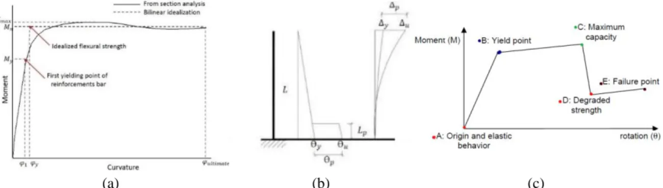
than two conducted to shear failures whereas columns with an aspect ratio greater than four failed in flexure mode. In this study all length/depth ratios of the columns are greater than four (Table 1), therefore the shear failure mechanism is not considered and it is assumed a flexure failure. A CC-S system in the longitudinal direction behaves as a cantilever structural system, and thus plastic hinges can only form at the bottom of the columns. However, in the transverse direction, the columns and cap beam form a frame-type system. In this case, plastic hinges can develop at both the top and bottom of the columns. CC-C bridge classes have a rigid connection between substructure and superstructure in both directions, and therefore concentrated plastic hinges based on the Caltrans recommendation (Caltrans 2013) are assigned to the bottom and top of the columns. Moment-curvature relationships describe the nonlinear behaviour of the elements. Fig. 4 shows a moment-curvature plot and an elastic-perfectly plastic idealization generated with the SAP2000 program (Computer and Structures Inc. 2009), which identifies the curvatures
corresponding to the damage states. The equivalent curvature (φy) corresponds to the relative
displacement of the column when the vertical reinforcing bars at the bottom of the column reach
the yield point. φy is obtained by extrapolating the line joining the origin and the point
corresponding to the first yielding point of a reinforcing bar up to the nominal moment capacity
Mn. Mn is the bending moment corresponding to εc=0.005, where εc is the compressive strain of a
concrete column (Priestley et al. 1987, Priestley et al. 1996). The curvature φy and Mn are the
moment at the section yield point on the idealized graph, given as
e n y EI M . This bilinear
representation was used to obtain φy and Mn; however, the numerical model considers the complete
moment-rotation relationship (Fig. 4(c)) to characterize the plastic hinge behaviour. Degradation in
pier strength happens when the maximum moment Mmax is reached.
Finally, concrete crushing occurs at the ultimate curvature (φultimate) when the concrete strain is
equal to εcu, where εcu is the compression strain corresponding to the rupture of the transverse
confining steel which calculated as '
cc su yh s cu f ε f p ε 0.0041.4 , however s D' A p h s 4
.The strain limit
can be calculated utilizing the energy balance approach (Mander et al. 1988). Note that fyh is the
yield strength of the transverse reinforcement, εsu is the steel strain at the maximum tensile stress,
f′cc is the compressive strength of the confined concrete, ρs is the volumetric ratio of confining
steel, Ah is the cross-sectional area of transverse reinforcement, D′ is the diameter of the confined
concrete core, and s is the longitudinal spacing of hoops or spirals. Since the curvature over the
plastic hinge length is assumed to be constant, the rotation angle can be determined as θ=φ×Lp.
Different proposals exist to estimate the hinge length (LP); in this research the expression proposed
by (Priestly et al. 1996) as follow: Lp=0.08L+0.022fyedbl≥0.044fyedbl, where fye is the yield strength
of the reinforcing bars and dbl is the diameter of the longitudinal reinforcing bars. Outside of the
plastic hinge length, the behaviour of the column is assumed to be linear. In order to quantify damage states, the relative displacement ductility ratio of a column is used. This variable is defined as:
1
Δ Δi i
μ , where μi= ductility demand at the ith damage state, Δi= relative displacement
at the top of a column at the corresponding limit state i and Δ1= relative displacement of a column
when the longitudinal reinforcing bars reach the first yield, calculated as follows: Δ1=
2 1 3 1 L , where (a) (b) (c)
Fig. 4 (a): Moment-curvature diagram of columns, (b): Distribution of a cantilever column curvature and displacement, (c): Plastic hinges behaviour in the nonlinear numerical model
L= the distance from the plastic hinge to the point of contra-flexure and φ1= the curvature
correspondent to the relative displacement of a column when the vertical reinforcing bars at the
bottom of the column reaches the first yield. Hence, µ1, denotes the first limit state corresponding
to a first yield displacement ductility ratio equal to 1. The second damage state, µy, represents the
yield displacement ductility ratio, calculated as:
1 2 1 3 Δ 1 Δ Δ L μ y y y
, where φy= the curvature
correspondent to the relative displacement of a column when the vertical reinforcing bars at the bottom of the column reaches the yield (Fig. 4(a)). The displacement ductility corresponding to the
third damage state which is nominated (µ2 or µ4) is the displacement ductility ratio corresponding
to εc=0.002 or εc=0.004 for the columns with or without lap splices, respectively, where εc is the
compressive strain at the concrete column (Hwang et al. 2001). Hence Δ3 can be estimated as
follow: ) 2 ( Δ Δ3 2 p p L L θ
, as which θp and Lp are the rotation and the plastic hinge length,
respectively. The plastic hinge rotation can be calculated as: θp=(φ3-φy)Lp, where φ3 is the
curvature of a column when εc=0.002 or εc=0.004 for the columns with or without lap splices,
respectively. Finally, forth damage state which is nominated µ2max or µ4max can be calculated as
follows: μ2max=μ2+3 or μ4max=μ4+3 (Hwang et al. 2001, FHWA 1995).
5. Ground motion selection
The seismic hazard level of earthquake ground motions can be identified by different ground motion intensity measures. The selected seismic records and intensity measures influence the reliability of bridge fragility curves. An appropriate correlation between seismic damages and hazard levels of ground motions is very important in the selection of intensity measures. PGA, peak ground velocity (PGV) and peak ground displacement (PGD) are examples of commonly used IMs. Optimal IMs selection can be supported by an examination of several characteristics of IMs that have been discussed by several studies (Baker 2005, Padgett et al. 2008, Iervolino et al. 2010, Bradley et al. 2015). In the study of Zelaschi et al. (Zelaschi et al. 2015) the analysis of RC bridges by providing a statistically sound comparison of analytical fragility curves due to traditional and innovative intensity measures of an extensive bridge is proposed. In the study of Buratti and Tavano (Buratti and Tavano 2014) by utilizing cloud analysis with a set of 40 recorded accelerograms, the sufficiency and efficiency of ground motion intensity is analysed. In particular, the peak ground displacement was founded the most efficient and sufficient intensity measure. In the study of Bradley et al. (Bradley et al. 2015) four methods were selected for dynamic seismic response analyses when the fundamental seismic hazard is quantified with ground motion simulation instead of empirical ground motion prediction equations. (Avsar 2009) analysed several ground motion intensity measures (ASI, PGV, PGA, and PGA/PGV). He found that ASI and PGV intensities have better correlation with the seismic damage of the bridge components. In the study of Padget et al. (Padget et al. 2008) it is noted that spectrally based quantities perform better correlation than PGA. Spectral accelerations at certain periods are employed as well (FEMA 2003, Nielson and DesRoches 2006).
In selecting the appropriate intensity measure, one of the most important principles is to account with the appropriate level of correlation between the hazard level of the ground motion and the degree of a constant seismic damage in the bridge. Therefore, the reliability of the fragility
curves is proportional to the selected intensity measure and the level of correlation with the seismic damage. Existing ground motion intensities can be directly calculated from ground motion records, such as peak ground acceleration (PGA). In this method PGA can be obtained directly from earthquake record databases without any additional information. Another intensity measure is based on the use of response spectrum of a ground motion for certain range of periods. Since PGA is one parameter with common applications in earthquake engineering, it is considered as representative for the first method investigated. However, the use of a single spectral acceleration could lead to unrealistic acceleration values that the bridge is expected to experience. The bridge acceleration level can be influenced by higher mode effects, therefore, by using spectrum intensity parameters, as a second approach, instead of considering a single period value, it is possible to deal with a period range over response spectra of the earthquake databases, and this approach can be more realistic (FEMA 2003, Nielson 2005). The area under an elastic response spectrum (5%
damped) between periods Ti and Tf is defined as the ASI with the following function:
f
i
T
T SAT,ξ dT
ASI ( ) (Von Thun et al. 1998, Yakut and Yılmaz 2008, Avsar et al. 2011), where Ti
and Tf are the initial and final periods of the interval. Based on modal analyses of the bridge
samples, fundamental period values vary between 0.36 and 1.38 s. In order to consider the higher mode effects and cover the elongated period of the bridge structure due to nonlinear actions,
periods Ti and Tf are selected as 0.3 and 1.45 s. The fundamental period for the CC-C bridges
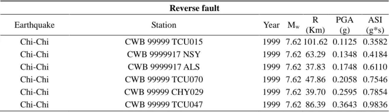
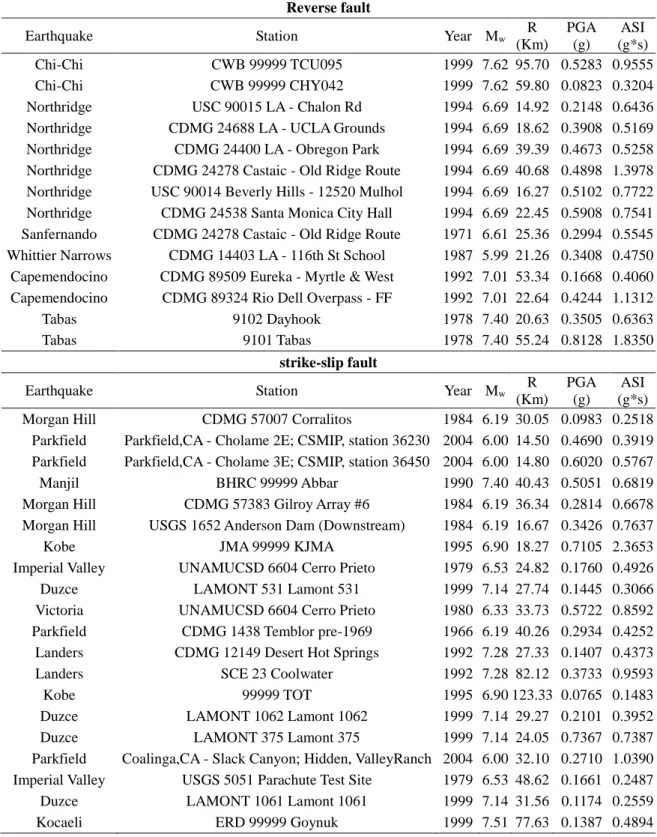
ranges from 0.36 to 0.73 s. This interval for CC-S bridges is between 0.99 and 1.38 s. Fig. 5 presents the response spectra and mean values of the selected earthquake ground motions with a 5% damping ratio, for reverse and strike-slip faults. Table 3 present some important features of the earthquakes selected and some characteristics of the ground motions. R is the epicentral distance. Earthquake mechanisms along active fault systems in Iran suggest the dominance of strike-slip faulting and reverse faulting. Due to the high density of active faults in Iran and the inaccuracy of the macro-seismic data of the area, the sources of some of the earthquakes have been related to more than one fault. Therefore, the development of studies on the seismic vulnerability of bridges based on different seismic sources seems to be necessary (Berberian 1994). Ground motions with PGA smaller than 0.05 g typically do not produce damages in bridges, and therefore seismic records with PGA<0.05 g were not considered. A suite of 104 earthquake ground motions satisfying the following conditions were selected: (a): all earthquake ground motions recorded in Iran, (b): ground motions recorded from other regions having the same seismic sources (strike-slip and reverse faulting mechanisms), (c): all bridges assumed to be recorded on hard soil, (d):
Table 3 Some important parameters of the selected earthquake ground motions Reverse fault
Earthquake Station Year Mw
R (Km) PGA (g) ASI (g*s) Chi-Chi CWB 99999 TCU015 1999 7.62 101.62 0.1125 0.3582 Chi-Chi CWB 9999917 NSY 1999 7.62 63.29 0.1348 0.4184 Chi-Chi CWB 9999917 ALS 1999 7.62 37.83 0.1748 0.6110 Chi-Chi CWB 99999 TCU070 1999 7.62 47.86 0.2058 0.7546 Chi-Chi CWB 99999 CHY029 1999 7.62 39.70 0.2595 0.7854 Chi-Chi CWB 99999 TCU047 1999 7.62 86.39 0.3643 0.9836
Table 3 Continued
Reverse fault
Earthquake Station Year Mw
R (Km) PGA (g) ASI (g*s) Chi-Chi CWB 99999 TCU095 1999 7.62 95.70 0.5283 0.9555 Chi-Chi CWB 99999 CHY042 1999 7.62 59.80 0.0823 0.3204
Northridge USC 90015 LA - Chalon Rd 1994 6.69 14.92 0.2148 0.6436 Northridge CDMG 24688 LA - UCLA Grounds 1994 6.69 18.62 0.3908 0.5169 Northridge CDMG 24400 LA - Obregon Park 1994 6.69 39.39 0.4673 0.5258 Northridge CDMG 24278 Castaic - Old Ridge Route 1994 6.69 40.68 0.4898 1.3978 Northridge USC 90014 Beverly Hills - 12520 Mulhol 1994 6.69 16.27 0.5102 0.7722 Northridge CDMG 24538 Santa Monica City Hall 1994 6.69 22.45 0.5908 0.7541 Sanfernando CDMG 24278 Castaic - Old Ridge Route 1971 6.61 25.36 0.2994 0.5545 Whittier Narrows CDMG 14403 LA - 116th St School 1987 5.99 21.26 0.3408 0.4750 Capemendocino CDMG 89509 Eureka - Myrtle & West 1992 7.01 53.34 0.1668 0.4060 Capemendocino CDMG 89324 Rio Dell Overpass - FF 1992 7.01 22.64 0.4244 1.1312
Tabas 9102 Dayhook 1978 7.40 20.63 0.3505 0.6363
Tabas 9101 Tabas 1978 7.40 55.24 0.8128 1.8350
strike-slip fault
Earthquake Station Year Mw
R (Km) PGA (g) ASI (g*s) Morgan Hill CDMG 57007 Corralitos 1984 6.19 30.05 0.0983 0.2518
Parkfield Parkfield,CA - Cholame 2E; CSMIP, station 36230 2004 6.00 14.50 0.4690 0.3919 Parkfield Parkfield,CA - Cholame 3E; CSMIP, station 36450 2004 6.00 14.80 0.6020 0.5767
Manjil BHRC 99999 Abbar 1990 7.40 40.43 0.5051 0.6819
Morgan Hill CDMG 57383 Gilroy Array #6 1984 6.19 36.34 0.2814 0.6678 Morgan Hill USGS 1652 Anderson Dam (Downstream) 1984 6.19 16.67 0.3426 0.7637
Kobe JMA 99999 KJMA 1995 6.90 18.27 0.7105 2.3653
Imperial Valley UNAMUCSD 6604 Cerro Prieto 1979 6.53 24.82 0.1760 0.4926
Duzce LAMONT 531 Lamont 531 1999 7.14 27.74 0.1445 0.3066
Victoria UNAMUCSD 6604 Cerro Prieto 1980 6.33 33.73 0.5722 0.8592 Parkfield CDMG 1438 Temblor pre-1969 1966 6.19 40.26 0.2934 0.4252 Landers CDMG 12149 Desert Hot Springs 1992 7.28 27.33 0.1407 0.4373
Landers SCE 23 Coolwater 1992 7.28 82.12 0.3733 0.9593
Kobe 99999 TOT 1995 6.90 123.33 0.0765 0.1483
Duzce LAMONT 1062 Lamont 1062 1999 7.14 29.27 0.2101 0.3952
Duzce LAMONT 375 Lamont 375 1999 7.14 24.05 0.7367 0.7387
Parkfield Coalinga,CA - Slack Canyon; Hidden, ValleyRanch 2004 6.00 32.10 0.2710 1.0390 Imperial Valley USGS 5051 Parachute Test Site 1979 6.53 48.62 0.1661 0.2487 Duzce LAMONT 1061 Lamont 1061 1999 7.14 31.56 0.1174 0.2559
(a) (b)
Fig. 5 Response spectra of the selected ground motions (5%damping), (a): reverse and (b): strike-slip faults
moment magnitude, Mw, varying between 5.99 and 7.62, (e): two horizontal orthogonal
components are considered in the nonlinear response history analyses. The earthquake ground
motions were downloaded from the strong motion database of PEER
(http://peer.berkeley.edu/smcat/) and COSMOS (http://db.cosmoseq.org/scripts/default.plx). The response spectrum of each ground motion is determined by taking the square root of the sum of the squares (SRSS) of the response spectrum of the two horizontal ground motion components. To select the ground motions, the distribution of ASI versus PGA of the accelerograms was evaluated. A small number of ground motions display high intensities, and accelerograms with low intensities impose limited seismic damages on the bridges. Therefore, we found impractical and time consuming to use all of the selected 104 ground motions for the response history analyses. A reduced set of data of ground motions based on each seismic source due to different levels of ASI and PGA was compiled. A total of 40 unscaled ground motions (20 recorded in reverse faults and 20 recorded in strike-slip sources) from Iran and other regions having similar faulting mechanisms and seismic potentiality were selected and shown in Table 3. Two horizontal orthogonal components are considered in the nonlinear response history analyses.
6. Development of fragility curves
Probabilistic methods are widely utilized to include structural uncertainties in the vulnerability assessment of bridges, based on live loading (O’Connor and Enevoldsen 2009) and seismic loading (Kim and Shinozuka 2004, Ramanathan et al. 2010). The expected seismic performance of a particular structure quantifies the potential for damage as a function of earthquake intensity (e.g., PGA). A probabilistic seismic performance analysis (PSPA), based on fragility curves, provides a framework to estimate the seismic behaviour and reliability of the structures (Ellingwood et al. 2004, Razzaghi and Eshghi 2014). Fragility functions determine the probability that the demand on a particular structure will reach or exceed its capacity as function of an earthquake intensity
measure. It can be expressed as follows: Fr=P[Sd≥Sc|IM]. where Fr is the fragility function, Sd is
the structural demand, Sc is the structural capacity, and IM is the ground motion intensity. The
The main objective of this study is to obtain fragility curves for two common bridge typologies in Iran with the presence of lap splices in columns, subjected to earthquakes from two seismic sources. The number of bridges that reach or exceed a specified damage limit state is determined by considering PGA and ASI as an intensity measures. The bridges are subjected to two orthogonal horizontal components of the ground motions. Since each bridge is analysed twice in both horizontal directions to obtain the maximum response (in the longitudinal and transverse directions), a total of 80 analyses are performed for each bridge. Based on the maximum ductility demand in columns, the damage limit state of the bridge is assessed due to Hwang et al. theory (Hwang et al. 2001, Mosleh et al. 2015). The ratio of the number of bridges that reaches or exceeds the specified damage limit state to the total number of sample bridges provides the probability of exceeding the corresponding limit state for a specific intensity. This process is performed for each ground motion and four damage limit states. Moreover, to reduce the jaggedness and to obtain smooth fragility curves for each bridge class, a mathematical expression is utilized. In recent studies, the cumulative lognormal probability distribution describes the probability of exceeding a certain damage limit state (FEMA 2003, Karim and Yamazaki 2003, Elnashai et al. 2004, Banerjee and Shinozuka 2007, Nielson and DesRoches 2007b). This study uses the lognormal distribution to obtain fragility curves as well. The exceedance probability values provide the median and dispersion values of the cumulative lognormal probability distribution function. The correlation between the fragility functions and probability points is
presented by a coefficient of correlation (R2), which varies between 0 and 1. More reliable
estimated fragility curves lead to R2values close to 1. Fragility functions of each bridge class for
the intensity measures PGA and ASI are performed considering the existence of lap splices in columns and different types of superstructures.
6.1 Lap splice
Hwang et al. (Hwang et al. 2001) proposed different damage limit states in columns to obtain fragility curves for critical bridge components. The presence of lap splices has a significant effect on the fragility curves, making the bridge more vulnerable to seismic effects. Hence, the placement of lap splices in critical locations of ductile elements is not permitted (FHWA 2006, AASHTO 2012, Caltrans 2013). However, old bridges may have lap splices near the column base that influence the damage limit states. Table 4 presents the relationship among four curvature demands
(φ1, φy,φ2, φ4) and displacement ductilities. The curvature for an extensive limit state depends on
the presence of column lap splices. θp2is the plastic hinge rotation of a column with lap splices for
a strain equal to 0.002 (εc=0.002). If the plastic hinge rotation is larger than this value (θp2), the
column core starts to disintegrate and bending failure happens. θp4 is the plastic hinge rotation
related to εc=0.004 for columns without lap splices (Hwang et al. 2001). The fragility curves for
two classes of bridges based on columns with and without lap slices were calculated.
Fig. 6 presents the fragility curves of the CC-S and CC-C bridges with and without lap splices, subjected to both groups of ground motions. These figures confirm that lap splices in longitudinal reinforcements should not be used in critical locations of ductile eleme nts (FHWA 2006, AASHTO 2012, Caltrans 2013). This figure displays extensive (LS3) and collapse (LS4) limit states because lap splices are only relevant in these cases. These results are relevant because the analyses correspond to real bridges. As an example of the influence of the lap splice and seismic source on the probability of reaching the limit states, Fig. 6(a) shows that, for PGA=0.5 g, the probabilities of reaching or exceeding LS3 subjected to the reverse fault records are 79 and 60%,
Table 4 Different levels of pier damage in function of the presence of lap splice, CC-C (8m) 0.0 0.2 0.4 0.6 0.8 1.0 0.0 0.2 0.4 0.6 0.8 1.0
LS3-with lap splice LS3-without lap splice LS4-with lap splice LS4-without lap splice
p ro b a b ili ty o f Excee d a n ce PGA (g) 0.0 0.2 0.4 0.6 0.8 1.0 0.0 0.2 0.4 0.6 0.8 1.0
LS3-with lap splice LS3-without lap splice LS4-with lap splice LS4-without lap splice
p ro b a b ili ty o f Excee d a n ce PGA (g) (a) (b) 0.0 0.2 0.4 0.6 0.8 1.0 0.0 0.2 0.4 0.6 0.8 1.0
LS3-with lap splice LS3-without lap splice LS4-with lap splice LS4-without lap splice
p ro b a b ili ty o f Excee d a n ce PGA (g) 0.0 0.2 0.4 0.6 0.8 1.0 0.0 0.2 0.4 0.6 0.8 1.0
LS3-with lap splice LS3-without lap splice LS4-with lap splice LS4-without lap splice
p ro b a b ili ty o f Excee d a n ce PGA (g) (c) (d)
Fig. 6 Fragility curves for different damage limit states (PGA) in function of the presence or not of lap splice in columns for two groups of classification, (a): CC-S-LS3&LS4-reverse fault, (b): CC-S-LS3&LS4-strike-slip fault, (c): CC-C-LS3&LS4-reverse fault, (d): CC-C-LS3&LS4-strike-CC-S-LS3&LS4-strike-slip fault
respectively. However, these values for LS4 decrease from 25 to 2%. In contrast, Fig. 6(b) indicates that the probabilities of reaching or exceeding LS3 are 70 and 58%, and for LS4 are 16 and 1% respectively. Fig. 6 also shows that seismic records from reverse faults make the bridges more vulnerable than the structures subjected to seismic records of strike-slips. It should be noted that the probability of reaching a specific limit state in CC-C bridges is higher than that probability in CC-S bridges. At low values of PGA, the differences between the graphs are large, but by increasing the PGA, the differences are reduced. This reflects that bridges with lap splice have more dispersed data. The different dispersion values approach both curves for high PGA values (LS3 and LS4) and eventually they can cross each other (LS3). The dispersion of data in LS4 limit state is not high enough to lead the graphs cross each other.
6.2 Effect of intensity measures on fragility curves
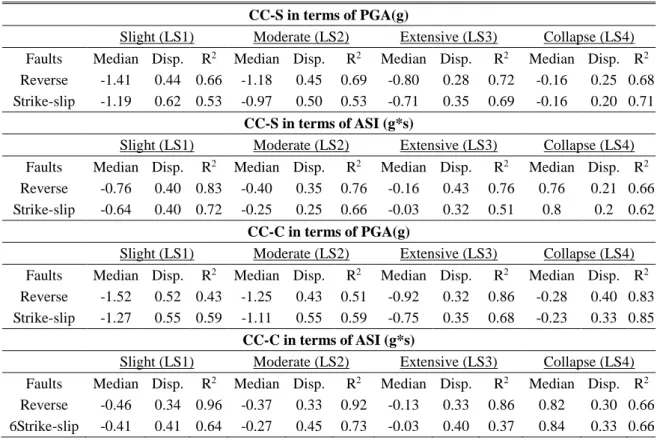
Table 5 shows the parameters of the lognormal density function used to obtain the fragility curves. The parameters depend on the seismic source and damage limit state. Median and
Table 5 Fragility curve parameters of the bridge classes
CC-S in terms of PGA(g)
Slight (LS1) Moderate (LS2) Extensive (LS3) Collapse (LS4) Faults Median Disp. R2 Median Disp. R2 Median Disp. R2 Median Disp. R2 Reverse -1.41 0.44 0.66 -1.18 0.45 0.69 -0.80 0.28 0.72 -0.16 0.25 0.68 Strike-slip -1.19 0.62 0.53 -0.97 0.50 0.53 -0.71 0.35 0.69 -0.16 0.20 0.71
CC-S in terms of ASI (g*s)
Slight (LS1) Moderate (LS2) Extensive (LS3) Collapse (LS4) Faults Median Disp. R2 Median Disp. R2 Median Disp. R2 Median Disp. R2 Reverse -0.76 0.40 0.83 -0.40 0.35 0.76 -0.16 0.43 0.76 0.76 0.21 0.66 Strike-slip -0.64 0.40 0.72 -0.25 0.25 0.66 -0.03 0.32 0.51 0.8 0.2 0.62
CC-C in terms of PGA(g)
Slight (LS1) Moderate (LS2) Extensive (LS3) Collapse (LS4) Faults Median Disp. R2 Median Disp. R2 Median Disp. R2 Median Disp. R2 Reverse -1.52 0.52 0.43 -1.25 0.43 0.51 -0.92 0.32 0.86 -0.28 0.40 0.83 Strike-slip -1.27 0.55 0.59 -1.11 0.55 0.59 -0.75 0.35 0.68 -0.23 0.33 0.85
CC-C in terms of ASI (g*s)
Slight (LS1) Moderate (LS2) Extensive (LS3) Collapse (LS4) Faults Median Disp. R2 Median Disp. R2 Median Disp. R2 Median Disp. R2 Reverse -0.46 0.34 0.96 -0.37 0.33 0.92 -0.13 0.33 0.86 0.82 0.30 0.66 6Strike-slip -0.41 0.41 0.64 -0.27 0.45 0.73 -0.03 0.40 0.37 0.84 0.33 0.66
dispersion values of the cumulative lognormal probability distribution function were calculated by
utilizing the least-squares technique. The coefficient R2 is also displayed to show the correlation
between the exceedance probability points and the fragility curves. Table 5 shows that ASI intensity measure has higher coefficient of determination than PGA for LS1 and LS2 limit states.
For example, CC-C bridges subjected to reverse fault records have R2 coefficients of 0.96 and 0.92
when using the ASI intensity measure for the slight and moderate limit states, respectively. However, these values are 0.43 and 0.51 when using PGA as the intensity measure. Fragility curves computed with the ASI intensity measure have a better correlation with exceedance probability points than the fragility curves developed by using PGA for the first two limit states.
6.3 Comparison of seismic performance of integral and simply supported superstructure types
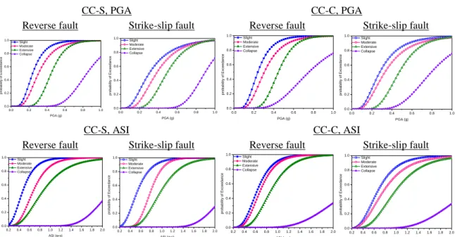
Fig. 7 shows the fragility curves for the two bridge classes subjected to reverse and strike-slip fault records using PGA and ASI as intensity measures. S bridges are less vulnerable than CC-C bridge models. This outcome is consistent with the bridge responses observed by previous researchers (Pan et al. 2010, Choine et al. 2015). The probability of exceeding extensive damage in an integral bridge is 80% for reverse fault records with PGA=0.5 g, whereas it is 70% in a simply supported bridge. One reason is that bearings reduce the transfer of inertial forces to the substructure (Frosch et al. 2009). The fundamental periods range from 0.36 to 0.73 s in CC-C
CC-S, PGA CC-C, PGA
Reverse fault Strike-slip fault Reverse fault Strike-slip fault
0.0 0.2 0.4 0.6 0.8 1.0 0.0 0.2 0.4 0.6 0.8 1.0 Slight Moderate Extensive Collapse p ro b a b ili ty o f Excee d a n ce PGA (g) 0.0 0.2 0.4 0.6 0.8 1.0 0.0 0.2 0.4 0.6 0.8 1.0 Slight Moderate Extensive Collapse p ro b a b ili ty o f Excee d a n ce PGA (g) 0.0 0.2 0.4 0.6 0.8 1.0 0.0 0.2 0.4 0.6 0.8 1.0 Slight Moderate Extensive Collapse p ro b a b ili ty o f Excee d a n ce PGA (g) 0.0 0.2 0.4 0.6 0.8 1.0 0.0 0.2 0.4 0.6 0.8 1.0 Slight Moderate Extensive Collapse p ro b a b ili ty o f Excee d a n ce PGA (g) CC-S, ASI CC-C, ASI
Reverse fault Strike-slip fault Reverse fault Strike-slip fault
0.2 0.4 0.6 0.8 1.0 1.2 1.4 1.6 1.8 2.0 0.0 0.2 0.4 0.6 0.8 1.0 Slight Moderate Extensive Collapse p ro b a b ili ty o f Excee d a n ce ASI (gs) 0.2 0.4 0.6 0.8 1.0 1.2 1.4 1.6 1.8 2.0 0.0 0.2 0.4 0.6 0.8 1.0 Slight Moderate Extensive Collapse p ro b a b ili ty o f Excee d a n ce ASI (gs) 0.2 0.4 0.6 0.8 1.0 1.2 1.4 1.6 1.8 2.0 0.0 0.2 0.4 0.6 0.8 1.0 Slight Moderate Extensive Collapse p ro b a b ili ty o f Excee d a n ce ASI (gs) 0.2 0.4 0.6 0.8 1.0 1.2 1.4 1.6 1.8 2.0 0.0 0.2 0.4 0.6 0.8 1.0 Slight Moderate Extensive Collapse p ro b a b ili ty o f Excee d a n ce ASI (gs) Fig. 7 Fragility curves for in terms of PGA and ASI subjected to reverse and strike-slip faults
bridge models and from 0.99 to 1.38 in CC-S bridge models. The fundamental periods of CC-S bridges locate the structures in a zone with smaller acceleration demands than those demands of the CC-C bridges.
The fragility curves show that both bridge classes are more vulnerable to reverse fault records. The probability of exceeding slight damage for PGA=0.5 g in CC-S bridges is 79% for strike-slip faults and 95% for reverse faults (Fig. 8(a)). The same behaviour is observed in other damage limit states, such as the moderate and extensive states, with increases of 71% to 86% and 52% to 65% for both seismic sources. Fig. 8(b) shows that the probability of exceeding slight damage for PGA=0.5 g in CC-C bridges increases from 85% to 95% for strike-slip and reverse faults, respectively. The same trend is observed for the moderate and extensive limit states, with increases
(a) (b)
Fig. 8 Fragility curves of the bridges subjected to reverse and strike-slip fault for different damage limit states in terms of PGA for (a): CC-S and (b): CC-C bridge classification
from 78% to 90% and from 55% to 75%. The probability of reaching the collapse limit state is about 5% for both seismic sources. It is also notable that the probability of reaching the slight damage state in both bridge models subjected to reverse fault records is 95%; conversely, the probabilities of reaching this damage state in the CC-S and CC-C bridges are 79 and 85%, respectively. Similar results were found for the moderate damage state. In general, the bridges subjected to the reverse fault records displayed larger demands than the bridges subjected to the strike-slip fault accelerograms. The fragility curves also show that concrete bridges present a low probability to reach collapse damage limit state for PGAs less than 0.4 g. This outcome is consistent with the bridge responses observed during past Iranian earthquakes that occurred in Manjil and Bam (Astaneh-Asl 1994, Zahrai and Heidarzadeh 2007, Manafpour 2008).
7. Conclusions
This study offers a comparison between the expected seismic performance of two common bridge classes in Iran based on PGA and ASI as intensity measures. The procedure obtains fragility curves based on 3-D analytical bridge models, a suite of ground motion records from reverse and strike faults, and full nonlinear response history analyses. Comparisons are also drawn between the seismic fragilities as function of the two seismic sources, using as a performance parameter the displacement ductility of the piers and damage limit states. The seismic performance of RC bridges is investigated, considering the continuity between substructure and superstructure and the presence of lap splices in columns. Results are important because this study considered existing bridges to obtain fragility curves that can be used to assess the potential losses resulting from earthquakes, retrofit prioritization strategies, and post-earthquake inspection decisions.
The results show that CC-S bridges perform consistently better than CC-C structures. However, RC columns of the integral bridges are more vulnerable to seismic damage than simply supported bridges. This is understandable considering that monolithic bridges transfer more demands from deck to columns when the bridge is seismically loaded. Another reason is related to the frequency content of the seismic records and the fundamental period of CC-C bridges, which ranges from 0.36 to 0.73 s, whereas the periods of CC-S bridges vary between 0.99 and 1.38 s. This study concentrates in damage limit states of pier columns, if superstructure unseating, collision between adjacent decks, abutments or other limit states had been considered, CC-S bridges could have been presented additional fragility curves.
It is also remarkable that bridges response is sensitive to the origin of the seismic ground motions. Bridges subjected to the reverse fault records displayed larger demands than bridges subjected to strike-slip fault accelerograms. The fragility curves showed that both bridge classes are more vulnerable to reverse fault records due to selected records.
Between the investigated ground motion intensity measures (ASI and PGA), ASI appeared to have a better correlation with the seismic damage sustained by bridge components for lower PGAs. Therefore, the fragility curves generated based on ASI was found to be more realistic in low damage states when estimating the damage limit states of the bridges.
The bridges with lap splices clearly exhibited higher seismic vulnerability than the bridge models without lap splices. The presence of lap splices had a significant effect on the fragility curves, making the columns more vulnerable to seismic effects. Old bridges with lap splices exhibited high seismic vulnerability. These structures must be carefully evaluated as candidates to be retrofitted to reduce the failure probability in future seismic events. The analyses of existing
bridges showed that more damage implies more influence of the lap splices. The presence of lap splices increases, from 60% to 79%, the probability of reaching or exceeding LS3 limit state for reverse fault records and PGA=0.5 g. However, the change is more important for LS4; in this case, the models with lap splices increase the probability of reaching or exceeding the limit state from 2% to 25%.
The developed fragility curves can be the basis of loss estimation models as well as the framework of retrofit prioritization strategies for bridges. The study shows that the bridges subjected to earthquakes originated on reverse faults are more vulnerable than the structures excited by strike-slip earthquakes. If the seismic hazard assessment of a region shows that a family of vulnerable bridges is located in a site where the seismic hazard is mainly governed by one of the seismic sources, the interventions should prioritize the structures affected by the reverse fault movements. However, if the bridges are located in the seismic zones with important contributions of both types of seismic sources, the interventions must be hierarchized by considering the bridges’ vulnerability, among other variables. The results of this study are limited to typical short- and medium-length RC bridges with failure mechanism governed by pier damages by preventing and retarding any possibility of bridge collapse related to other bridge components. This study determined numerically the dynamic properties of the bridges, experimental vibration measurements could improve the calibration of the finite element models.
References
AASHTO (2012), AASHTO LRFD Bridge Design Specifications, American Association of State Highway and Transportation Officials. Washington, D.C., USA.
Astaneh-Asl, A. (1994), Lessons of the 1990 Manjil-Iran Erathquake, Paper presented at the Tenth world conference Balkema, Rotterdam.
ATC (1985), Earthquake Damage Evaluation Data for California, Report No. ATC-13. Retrieved from Applied Technology Council.
Aviram, A., Mackie, K.R. and Stojadinovic, B. (2008), Guidelines for Nonlinear Analysis of Bridge Structures in California, Retrieved from PEER Report 2008/03 Pacific Earthquake Engineering Research Center.
Avsar, O. (2009), “Fragility based seismic vulnerability assessment of ordinary highway bridges in Turkey”, Doctor of Philosophy, Middle East Technical University.
Avsar, O., Yakut, A. and Caner, A. (2011), “Analytical fragility curves for ordinary highway bridges in Turkey”, Earthq. Spectra, 27(4), 971-996.
Avsar, O. and Yakut, A. (2012), “Seismic vulnerability assessment criteria for RC ordinary highway bridges in Turkey”, Struct. Eng. Mech., 43(1), 127-145.
Baker, J.W. (2005), Vector-valued Ground Motion Intensity Measures for Probabilistic Seismic Demand Analysis, Retrieved from U.S.
Banerjee, S. and Shinozuka, M. (2007), “Nonlinear static procedure for seismic vulnerability assessment of bridges”, Comput.-Aid. Civ. Infrastruct., 22(4), 293-305.
Basoz, N. and Kiremidjian, A.S. (1997), Evaluation of Bridge Damage Data From the Loma Prieta and Northridge CA Earthquakes, (Report No. MCEER-98-0004). Retrieved from Buffalo, NY: MCEER, University at Buffalo, The State University of New York.
Bazant, Z.P. and Bhat, P.D. (1976), “Endochronic theory of inelasticity and failure of concrete”, J. Eng. Mech. Div., 102(4), 701-722.
Berberian, M. (1994), “Natural Hazard and the First Earthquake Catalogue of Iran”, Historical Hazards in Iran Prior to 1900 (Vol. 1).
Billah, A. and Shahria Alam, M. (2015), “Seismic fragility assessment of highway bridges: a state-of-the-art review”, Struct. Infrastruct. Eng., 11(6), 804-832.
Billah, A. and Shahria Alam, M. (2016), “Performance-based seismic design of shape memory alloy-reinforced concrete bridge piers. I: Development of performance based damage states”, J. Struct. Eng., 04016140.
Billah, A., Shahria Alam, M. and Bhuiyan, A.R. (2013), “Fragility analysis of retrofitted multi-column bridge bent subjected to near fault and far field ground motion”, J. Bridge Eng., ASCE, 18(10), 992-1004. Bojórquez, E., Iervolino, I., Reyes-Salazar, A. and Ruiz, S.E. (2012), “Comparing vector-valued intensity
measures for fragility analysis of steel frames in case of narrow-band ground motions”, Eng. Struct., 45, 472-480.
Bradley, B.A., Burks, L.S. and Baker, J.W. (2015), “Ground motion selection for simulation-based seismic hazard and structural reliability assessment”, Earthq. Eng. Struct. Dyn., 44(13), 2321-2340.
Buratti, N. and Tavano, M. (2014), “Dynamic buckling and seismic fragility of anchored steel tanks by the added mass method”, Earthq. Eng. Struct. Dyn., 43(1), 1-21.
Caltrans (2013), Seismic Design Criteria Version 1.7. California Department of Transportation, Sacramento, CA.
Choi, E., DesRoches, R. and Nielson, B. (2004), “Seismic fragility of typical bridges in moderate seismic zones”, Eng. Struct., 26(2), 187-199.
Choine, M., Connor, A. and Padgett, J. (2015), “Comparison between the seismic performance of integral and jointed concrete bridges”, J. Earthq. Eng., 19(1), 172-191.
Computers and Structures Inc., CSI. SAP2000 V-14 (2009), “Integrated finite element analysis and design of structures basic analysis reference manual”, Berkeley, CA, USA.
Denton, S. and Tsionis, G. (2012), “The evolution of Eurocodes for bridge design European commission”, Joint Research Centre, Institute for the Protection and Security of the Citizen, Luxembourg.
Der Kiureghian, A. (2002), “Bayesian methods for seismic fragility assessment of lifeline components”, Eds.,Taylor, C. and VanMarcke, E., Acceptable risk processes: lifelines and natural hazards, ASCE council on disaster reduction and technical council on lifeline earthquake engineering monograph, 21, 61-77. Dutta, A. and Mander, J.B. (1998), “Seismic Fragility Analysis of Highway Bridges”, Tokyo, Japan. Ellingwood, B.R., Rosowsky, D.V., Li, Y. and Kim, J.H. (2004), “Fragility assessment of light-frame wood
construction subjected to wind and earthquake hazards”, J. Struct. Eng., 130(12), 1921-1930.
Elnashai, A., Borzi, B. and Vlachos, S. (2004), “Deformation-based vulnerability functions for RC bridges”, Struct. Eng. Mech., 17(2), 215-244.
Eshghi, S. and Razzaghi, M.S. (2004), “The behavior of special structures during the Bam earthquake of 26 December 2003”, J. Seismol. Earthq. Eng., 5(4), 197-207.
FEMA (2003), HAZUS-MH MR1: Technical Manual, Vol. Earthquake Model, Washington D.C. Federal Emergency Management Agency.
FHWA (1995), Seismic Retrofitting Manual for Highway Bridges Publication No.FHWA-RD-94-052, Office of Engineering and Highway Operations R&D, Federal Highway Administration, McLean, VA.
FHWA (2006), Seismic Retrofitting Manual for Highway Structures Federal Highway Administration: Report No. FHWA-HRT-06-032.
Frosch, R.J., Kreger, M.E. and Talbott, A.M. (2009), “Earthquake resistance of integral abutment bridges”, Retrieved from Publication No. FHWA/IN/JTRP-2008/11, SPR-2867.
Gehl, P. and Ayala, D.D. (2016), “Development of Bayesian Networks for the multi-hazard fragility assessment of bridge systems”, Struct. Safety, 60, 37-46.
Hedayati Dezfuli, F. and Shahria Alam, M. (2016), “Effect of different steel-reinforced elastomeric isolators on the seismic fragility of a highway bridge”, Struct. Control Hlth. Monit., doi: 10.1002/stc.1866. Hwang, H., Jernigan, J.B. and Lin, Y.W. (2000), “Evaluation of seismic damage to Memphis bridges and
highway systems”, J. Bridge Eng., ASCE, 5(4), 322-330.
Hwang, H., Liu, J. and Chiu, Y. (2001), “Seismic fragility analysis of highway bridges”, Center for Earthquake Research and Information The Universityof Memphis, MAEC RR-4 Project.
intensity measures”, Bull. Seismol. Soc. Am., 100(6), 3312-3319.
Lin, Z., Yan, F., Azimi, M., Azarmi, F. and Al-Kaseasbeh, Q. (2015), “A revisit of fatigue performance based welding quality criteria in bridge welding provisions and guidelines”, Shaanxi, China.
Lin, F., Azarmi, F., Al-Kaseasbeh, Q. and Azimi, M. (2015), “Advanced ultrasonic testing technologies with applications to evaluation of steel bridge welding an overview”, Appl. Mech. Mater., 727, 785-789. Jara, J.M., Jara, M., Hernández, H. and Olmos, B.A. (2013a), “Use of sliding multirotational devices of an
irregular bridge in a zone of high seismicity”, KSCE J. Civ. Eng., 17(1), 122-132.
Jara, M., Jara, J.M. and Olmos, B.A. (2013b), “Seismic energy dissipation and local concentration of damage in bridge bents”, Struct. Infrastruct. Eng., 9(8), 794-805.
Jeon, J., Shafieezadeh, A., Lee, D., Choi, E. and DesRoches, R. (2015), “Damage assessment of older highway bridges subjected to three-dimensional ground motions: Characterization of shear-axial force interaction on seismic fragilities”, Eng. Struct., 87, 47-57.
Karim, K.R. and Yamazaki, F. (2003), “A simplified method of constructing fragility curves for highway bridges”, Earthq. Eng. Struct. Dyn., 32(10), 1603-1626.
Kent, D.C. and Park, R. (1971), “Flexural members with confined concrete”, J. Struct. Div., 97, 1969-1990. Kim, S.H. and Shinozuka, M. (2004), “Development of fragility curves of bridges retrofitted by column
jacketing”, Prob. Eng. Mech., 19(1), 105-112.
Loh, C.H., Liao, W.I. and Chai, J.F. (2002), “Effect of near-fault earthquake on bridges: lessons learned from Chi-Chi earthquake”, Earthq. Eng. Eng. Vib., 1(1), 86-93.
Manafpour, A.R. (2008), “Bam Earthquake, Iran: Lessons on The Seismic Behavior of Building Structures”, The 14th World Conference on Earthquake Engineering Beijing, China.
Mander, J.B., Priestley, M.J.N. and Park, R. (1988), “Observed stress strain behavior of confined concrete”, J. Struct. Eng., 114(8), 1827-1849.
Maroney, B.H. (1995), “Large Scale Abutment Tests to Determine Stiffness and Ultimate Strength Under Seismic Loading”, Ph.D. Dissertation, University of California, Davis, CA.
Mistry, V.C. (2005), “Integral Abutment and Jointless Bridges Paper presented at the THE 2005 - FHWA CONFERENCE Integral Abutment and Jointless Bridges (IAJB)”, Baltimore, Maryland.
Mollaioli, F., Lucchini, A., Cheng, Y. and Monti, G. (2013), “Intensity measures for the seismic response prediction of base-isolated buildings”, Bull. Earthq. Eng., 11(5), 1841-1866.
Monti, G. and Nistico, N. (2002), “Simple probability-based assessment of bridges under scenario earthquakes”, J. Bridge Eng., 7(2), 104-114.
Mosleh, A. (2016), “Seismic vulnerability assessment of existing concrete highway Iranian bridges”, Doctor of Philosophy, Aveiro University.
Mosleh, A., Razzaghi, M.S., Jara, J. and Varum, H. (2016a), “Seismic fragility analysis of typical Pre-1990 bridges due to near and far-field ground motions”, Int. J. Adv. Struct. Eng., 8(1), 1-9.
Mosleh, A., Varum, H. and Jara, J. (2015), “A methodology for determining the seismic vulnerability of old concrete highway bridges by using fragility curves”, J. Struct. Eng. Geotech., 5(1), 1-7.
Mosleh, A., Rodrigues, H., Varum, H., Costa, A. and Arêde, A. (2016b), “Seismic behavior of RC building structures designed according to current codes”, Structures, 7, 1-13.
Nateghi, F. and Shahsavar, V.L. (2004), “Development of fragility and reliability curves for seismic evaluation of a major prestressed concrete bridge”, The 13th World Conference on Earthquake Engineering, Vancouver, B.C., Canada.
Nicknam, A., Mosleh, A. and Hamidi, H. (2011), “Seismic performance evaluation of urban bridge using static nonlinear procedure, case study: hafez bridge”, Procedia Eng., 14, 2350-2357.
Nielson, B.G. and DesRoches, R. (2006), “Seismic fragility methodology for highway bridges using a component level approach”, Earthq. Eng. Struct. Dyn., 36(6), 823-839.
Nielson, B.G. (2005), “Analytical fragility curves for highway bridges in moderate seismic zones”, Ph.D. Thesis, Atlanta, Georgia.
Nielson, B.G. and DesRoches, R. (2007a), “Analytical seismic fragility curves for typical bridges in the Central and Southeastern United States”, Earthq. Spectra, 23(3), 615-633.