Scalable analysis of multitemporal images using an array database

(1)

Scalable Analysis of Multitemporal Images Using an Array

Database

Abhasha Joshi

Research Report Submitted in Partial Fulfillment of the Requirements for the Degree of Master of Science in Geospatial Technology

(2)

i

Scalable Analysis of Multitemporal Images Using an

Array Database

By: Abhasha Joshi

Research Report submitted in partial fulfillment of the requirements for the degree of Master of Science in Geospatial Technology

Date: February 24, 2017

Supervised by:

Prof. Dr. Edzer Pebesma

Institute for Geoinformatics (ifgi) University of Muenster

Muenster, Germany

Co-supervised by:

Prof. Dr. Roberto Henriques NOVA - Information Management School (NOVA IMS)

Universidade Nova de Lisboa Lisbon Portugal

Co-supervised by: Marius Appel

Institute for Geoinformatics (ifgi) University of Muenster

(3)

ii

Declaration

I hereby declare that I am the sole author of this Master Thesis entitled “Scalable Analysis of Multitemporal Images using an Array Database”.

I declare that this thesis is submitted in support of candidature for the Master of Science in Geospatial Technologies and that it has not been submitted for any other academic or non-academic institution.

Abhasha Joshi

(4)

iii

Acknowledgements

I want to sincerely thank Prof. Dr. Edzer Pebesma, Prof. Dr. Roberto Henriques and Marius Appel for providing me the opportunity to carry out this research and supervising it. Their valuable advice, critical comments, and constant guidance made the smooth running of the study possible.

Some of the technologies used in this study were beyond my area of expertise and it was necessary to learn them. Marius showed great patience and willingness to share these concepts. I can honestly say without his help I would not be able to direct the thesis properly.

I also express thanks to Dr. Carl Schultz, Prof. Dr. Christoph Brox, Prof. Dr. Christian Kray and Prof. Dr. Marco Painho for their guidance and support.

My sincere thanks go to Erasmus Mundus Program of the European Commission for providing me a scholarship to accomplish the Master‟s program.

I would also like to thank all of the staff at Universitat Jaume I and the University of Muenster for the wonderful study experience.

Finally, I want to thank all my friends with whom, I had the privilege of studying together in this Master‟s program.

(5)

iv

Abstract

Massive archives of earth observation data are now available and the size of this data is increasing at a tremendous rate. This data is a very important resource and has a variety of applications including monitoring change, forestry application, agricultural application and urban planning. At the same time, they also possess challenge of storage, management, and high computational needs.

In this study SciDB, an array-based database is used to store, manage and process multitemporal satellite imagery. The major aim of this study is to investigate the performance of SciDB based scalable solution to run arithmetic operation, simple time series analysis and complex time series analysis on multitemporal satellite imagery.

This study provides better insight of SciDB architecture and provides suggestions for better performance in SciDB for remote sensing jobs. The research also compared the performance of time series analysis on SciDB array with file-based analysis using multicore parallelization (Using „Parallel‟ Package of R). It is found that SciDB provides a faster solution for time series analysis. However, SciDB might not be the best solution if the data size is smaller. Also, relative immaturity of SciDB and limited inherent support of remote sensing operations increases effort for the scientist to develop SciDB based solution. Nevertheless, SciDB has the potential to meet the ever increasing storage, management and computational need of big remote sensing data.

(6)

v

Keywords

Array Database SciDB

High Performance Computing Remote Sensing

(7)

vi

List of Figures

Figure 1 Basic SciDB architecture ... 7

Figure 2 Multitemporal Images as SciDB Array ... 8

Figure 3 Multitemporal Images stack ... 9

Figure 4 Location of the Data ... 12

Figure 5 Workflow of operations ... 15

Figure 6 Subset of NDVI array visualized ... 20

Figure 7 Cells processed per second for NDVI computation ... 22

Figure 8 Maximum NDVI array visualized ... 23

Figure 9 Time series processed per second for maximum NDVI computation ... 25

Figure 10 Change Magnitude from BFAST monitoring... 26

Figure 11 Breakpoint detected by BFAST Monitor with year ... 27

Figure 12 Time series processed per second for BFAST monitor query in SciDB ... 29

Figure 13 Comparison of processing time in raster file and SciDB array ... 31

Figure 14 Speed up of SciDB over file system ... 32

List of Tables

Table 1 Specification of Image Used. ... 13

Table 2 Size of Data Window ... 14

Table 3 Number of SciDB instances and CPU cores ... 14

Table 4 Time for upload and restructuring data in SciDB ... 17

Table 5 Performance metric for NDVI computation ... 21

Table 6 Performance metrics for max NDVI computation ... 24

Table 7 Performance Metrics for BFAST monitoring function in SciDB ... 29

Table 8 Performance Metrics for BFAST monitoring function in Raster file ... 30

(10)

1

Introduction

Chapter 1:

Background and Motivation

1.1.

The massive amount of earth observation data is now available in the archives which have been collected by different sensors for a long time. Currently, this data is increasing at an exceptionally fast rate with the advent of the new sensor with varied spectral, spatial and temporal resolutions. National imagery archives are storing terabytes of data every day and total stored imagery volume will grow to the order of Exabyte (OGC, 1999). These remote sensing data of large part of the world is big wealth to model the earth. It can be used to monitor environmental events, monitor natural disasters and study climate change. Other application area includes forestry, urban planning, land management, food security. However, these Big Remote Sensing (RS) data also poses the significant challenge of management, processing, and interpretation (Ma, et al., 2015). Recent research trends show the development of processing techniques for these data, such as time series processing methods to detect change (Verbesselt, Zeileis, & Herold, 2012), identify land cover (Clark, et al., 2010). However, there is the big challenge in managing these data and fulfill high computation requirement to process them.

Generally, these RS big data are stored in files and most scientific data analysis methods for these data are file-based. But as the volume of the data increases, arises the problem of not only data management but also of computational resource. Scientific community demands for the development of novel way in order to manage these enormous data and support distributed computation.

Relational database management systems (RDBMS) have been successful in addressing storage and analysis requirement of the varied business world from a long time. However, RDBMS are showing limitation when there is need of horizontal scalability and distributed computation (Jacobs, 2009), which is an essential requirement for RS data. Moreover, RS data has an array like structure and it is advantageous to store the data in an array structure, to perform many RS operations.

(11)

2

Cudre-Mauroux et al. (2010) demonstrate that the array-based database outperforms mature MySQL database for analysis array like Astronomical data. Thus array-based database with distributed storage and distributed computation has potentialities to manage and process big RS data.

SciDB is an open source multidimensional array based database and supports distributed storage, parallel processing, sparse array storage and user defined function and data types (Stonebraker, Brown, Poliakov, & Raman, 2016). Some of the recent studies suggest prospective of SciDB in RS applications. Planthaber et al. (2012) successfully tested SciDB to store and perform basic analysis on Modis Level 1 data. Appel & Pebesma (2016) have demonstrated an approach to remote sensing analysis using SciDB in an easy and reproducible way.

In this context, in this research, we intend to store and process multitemporal remote sensing data in SciDB and run a benchmark to analyze its performance.

Aims and Objectives

1.2.

Processing large volume of multitemporal satellite imagery is a computationally intensive process. In this study, a scalable solution shall be designed and implemented using SciDB array-based database to meet the high computational requirement of such data. The performance of the solution shall be explored and compared with a file-based image processing technique. Thus the primary aim of this research is to investigate the performance of SciDB based scalable solution for analysis of multitemporal satellite imagery.

The major objectives are to:

 Demonstrate applicability of SciDB to store, manage and analyze multitemporal remote sensing imagery

 Investigate the performance of SciDB in a different number of server instances, CPU cores, and data window.

 Compare the performance of time series analysis on SciDB array with the analysis in raster file parallelized by the multi-core support using „Parallel‟ package of R.

(12)

3

Thesis

Organization/ Structure

1.3.

This thesis is organized into 6 chapters. This (Introduction) chapter provides background, motivation aims and objectives for this study. Chapter 2 reviews existing work in the field and provide a theoretical base for the study. Chapter 3 describes the methodological approach and provides design decisions and implementation in details. Chapter 4 provides findings of the experiment. Chapter 5 tries to infer the result and discuss reason and meaning of different results obtained. Finally, chapter 6 summarizes the finding of the research, concludes thesis and provides suggestions for further research in the similar direction. There are also three appendices: Appendix A: Server Specification, Appendix B: SciDB Configuration and Appendix C: Code.

(13)

4

Literature Review

Chapter 2:

This chapter aims to present the theoretical basis for the study. Remote sensing big data is explained in the subsection 2.1. Existing works in High Performance Computing (HPC) techniques to meet the computational requirement of such big RS data is summarized next. Then we explain about R, an analytical programming language and its application as HPC technique in RS. Then in section 2.4, we describe in brief about SciDB which is the array database used in this study. Different kind of analysis can be performed in RS data. Time series analysis is a widely used method to get meaningful information from multitemporal imagery. Finally, different time series analysis for multitemporal RS data is described in brief in the last subsection.

Big Earth Observation Data

2.1.

Laney (2001) defined big data for the first time as data characterized by the 3Vs: Volume, Velocity, and Variety. The big data are shifting research paradigm to data-driven research (Kitchin, 2014). They are a source of innovation and productivity. Remote Sensing data can be indisputably termed as big data. The size of the image in archives is of multiple petabytes and these data are increasing at a rapid rate with the addition of sensors with a frequent revisit. Also, these data varies in terms of their spatial, spectral and radiometric resolution, coordinate system, format, and information they store. There is the great potential of using remote sensing big data in a variety of field. The data is the archived models of earth of different time. Some of the applications are monitoring of natural events, tracking of environmental changes, agricultural study, forestry etc.

The major challenges of any big data include building the storage system, running computation, visualizing the data and validating it (Li, et al., 2016). Research are increasingly being focused on addressing those challenges. Among those challenges, we are interested in massive storage need and high computing requirements of RS big data in this study.

(14)

5

High Performance Computing in RS

2.2.

High Performance Computing is the use of computing power in such a way that it provides higher performance than a traditional desktop for running advanced application programs efficiently, reliably and quickly. One of the major applications of future-generation HPC is big data analytics (Kambatla, et al., 2014). Lee et al. (2011) summarized recent HPC techniques for RS into mainly three classes, i.e. programmable hardware, multi-processor systems and distributed networks. Use of a graphics processing unit (GPU) together with a CPU to accelerate processing falls in the first category. Lately, GPUs have developed into highly parallel, multithreaded, many-core processors with huge computational capacity and high memory bandwidth (Nickolls & Dally, 2010). Ma et al. (2014) and Liu et al. (2011) have adopted multi-core cluster based HPC in a number of remote sensing applications. This kind of scaling up uses multi-core architecture in the context of a single application and is often done through multi-threading and in-process message passing. The third class of HPC is distributed computing, which is done by distributing jobs across machines over the network.

R for HPC in Remote Sensing

2.3.

R (R Core Team, 2016) is an open source data analysis programming language. It is also one of the most popular languages for data analytics. (Piatetsky, 2017) . R is highly extensible through the use of packages. A package is a library of functions of a specific field of study.

To support big data paradigm, research during the last decade has explored using HPC techniques with R. The packages that support parallel computing and HPC technique with R are listed in HPC Task View page (Eddelbuettel, 2017).

Parallel package of R is built upon work of the packages multicore and snow and is available inside r-core ( R Core Team(b), 2016). It provides functions for parallel execution of R code on machines with multiple cores or CPUs. The computation in this package starts with setting up a collection of “workers” that will be doing the job. The number of workers should ideally be one per core. Then the function in this

(15)

6

package divides work into equally sized chunks and sends the chunk to the worker. Principally different chunks of computation are unrelated and do not need to communicate in any way.

Raster package is a very powerful tool for remote sensing analysis in R and is extensively being used. Many other packages are also available for remote sensing analysis which are built over raster packages. For time-consuming remote sensing operation, it is efficient to run them in parallel. To parallelize work in multiple cores remote sensing job has to be divided into multiple independent chunks and then process them in each core. RStoolbox (Leutner & Horning, 2017), BfastSpatial (Dutrieux, 2016) , Modis (Mattiuzzi, et al., 2017) are some of the remote sensing packages that use the parallel package to parallelize work in multiple cores. This technique can be categorized as multi-processor systems HPC in Lee et al. (2011) „s classification.

SciDB

2.4.

SciDB is an open-source, array-based database, tailored towards the management needs of scientists. (Stonebraker, Brown, Poliakov, & Raman, 2016). Data in SciDB are stored in an n-dimensional sparse array. SciDB array is created by specifying its dimensions and attributes of the array. For example a 3-dimensional SciDB array may have x, y and z dimensions with values (0,1,2,…,20),(1,2,3,…,50) and (alfa,beta,…) respectively. Each combination of dimension values defines a cell .Cells in the array contain tuple of values, each of which is called as an attribute. For example a1,a2,a3,a4 can be name for four different attributes for each cell.

SciDB arrays are stored in one or more instances which can reside on a single server or distributed along the clusters allowing distributed storage and parallel processing. SciDB runs on a grid of computers and follows shared nothing architecture. Each SciDB instance and is responsible for local storage and processing and has sole access to the respective data. Thus scalability for big data is possible in SciDB because of its shared-nothing engine. SciDB array-based computing can be categorized as distributed network HPC in Lee et al. (2011) „s classification.

(16)

7

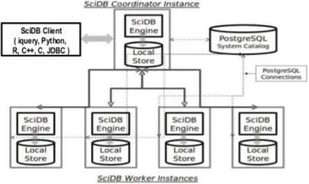
. The basic architecture of SciDB is shown in figure 1.

Figure 1 Basic SciDB architecture (SciDB User's Guide, 2013)

While all the available SciDB instance in cluster participate in storage and query processing; only one instance is used to connect and communicate to an external application. One of the instances is the coordinator instance and is responsible for facilitating all interaction between the SciDB external client and the entire SciDB database. The rest of the system instances work for the coordinator for query processing.

SciDB divides the data into smaller portions called chunk and each SciDB instance is responsible for storing and running queries on chunk (SciDB User's Guide, 2013). Because of this uniform distribution of storage and workload SciDB is able to deliver scalable performance on very large data sets. The user only has to specify chunk size for chunking. Each dimension of an array is divided into chunks of specified length. SciDB also follows vertical portioning to store multiple attributes in an array. That mean each attribute is stored in different chunks. It is recommended to select chunk size such that each chunk contains roughly 10 to 20 MB of data. It is necessary to consider vertical partitioning when selecting the chunk size. The number of attributes

(17)

8

of the array does not determine the chunk size rather the number of cells determines it.

SciDB is currently supported only on Linux operating system. Interaction with SciDB server is done through iquery which is default SciDB client or by language binding using R or python. Two languages are available in SciDB: Array Query Language (AQL) and Array Functional Language (AFL). AQL is SQL-like query language whereas AFL is a functional language for SciDB. AQL is compiled into AFL.

SciDB has limited analysis capability but it can be extended using plugins that allow running script of powerful analytic language R and python inside SciDB array. R_exec (Lewis, 2016) plugin of SciDB provides a way to run R script inside SciDB queries. The script can run in all SciDB chunks independently allowing parallel processing. It is necessary to adjust the chunk shape and size based on the analysis for using the r_exec function for analysis. The r_exec function only takes double data as input and the output of the r script should be list data type. This list can then be saved as a SciDB array.

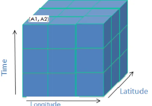
The multitemporal image in SciDB can be stored along three dimensions representing longitude, latitude and time. Its attributes can be different bands of the image. It is analogous to stacking up multitemporal images one above other. The data retrieved by keeping longitude and latitude constant is the time series of that location. Figure 2 presents a schema for storage of multitemporal images in SciDB and figure 3 shows it‟s analogous in the file system.

(18)

9

Figure 3 Multitemporal Images stack (Source: mdpi.com)

An array-based database provides better flexibility for managing and analyzing remote sensing images than the traditional relational database solutions (Tan & Yue, 2016). An array is the natural model for remote sensing data and simulating array data on top of tables is an unnatural act and usually results in poor performance (Stonebraker, Brown, Zhang, & Becla, 2013). Most of the operation in RS data like machine learning, k-nearest neighbors, spatial smoothing, Fourier transforms, regridding are operations over the array and run faster in array implementation but need relational data to be cast into arrays for processing. Further array database allows to subset the data and perform complex analysis without changing the data model. SciDB has been found better than SQL database to retrieve data from multiple overlapping images as in the case of time series image or hyperspectral image (Hausen, 2016).

Time Series Analysis

2.5.

Time series analysis on remote sensing can be done for various purposes such as to detect change, identify land cover and study crop growth. Break for Additive Seasonal and Trend (BFAST) allow “detection and characterization” of change in time series (Verbesselt, Hyndman, Newnham, & Culvenor, 2010). Other methods for change analysis include Principal Component Analysis (PCA) (Crist & Cicone, 1984),

(19)

10

wavelet decomposition (Anyamba & Eastman, 1996) and Fourier analysis (Azzali and Menenti, 2000).

Jan Verbesselt et al. in 2012 introduces BFAST monitor, an approach for monitoring time series data based on a BFAST-type season-trend model (Verbesselt, Zeileis, & Herold, 2012), that is applicable to different types of time. The BFAST monitoring splits time series data into history and monitoring period. From the data of historical period, it detects and models the stable history in order to detect disturbances within newly acquired data. Different models are available for modeling the stable historical behavior. Also to determine the size of the stable history period, different methods are available. It can be set based on subject-matter knowledge, data-driven methods or Reverse-ordered CUSUM test (ROC).

The simpler statistical method of time series analysis includes the mean, median, maximum, minimum value of some indices. The maximum, minimum or median value of time series Normalized difference vegetation index (NDVI) are also input to other indices which state vegetation condition at a particular time such as Vegetation Condition Index(VCI), Mean Referenced Vegetation Condition Index (MVCI), NDVI Change Ratio etc. VCI relates the present NDVI to the range of values observed in the same period in previous years. MVCI is NDVI percent change ratio to historical time series mean NDVI. Similarly, NDVI Change Ratio to Median can also be computed. These indices give an idea where the observed value is situated compared to central value or range of observed value.

The problem with implementing time series analysis methods is some of them are very computationally intensive. For example running BFAST in a normal computer in serial over a Landsat scene of 10 years can even take around a week. When the data size increases it becomes impossible to process them in desktop or even in high performing single servers. Thus it is crucial to use such processing methods inside high performance computing environment.

(20)

11

Methodology

Chapter 3:

Design Consideration

3.1.

In this research, we implemented analysis technique for big RS data inside array-based database environment and analyzed how the system performs. This research is designed to qualitatively demonstrate an approach for management and analysis of multitemporal images and quantitatively highlight performance and scalability of SciDB for analysis of the multitemporal image.

We designed the benchmark that includes queries to perform arithmetical operations, simple time series analysis and complex time series analysis on the image within SciDB. The benchmark was designed to test the performance of the system with changing data load, SciDB instances and CPU cores. The performance of the system was assessed based on the response time for a fixed task.

Furthermore, we also compared the result of the complex time series analysis in SciDB with time to do the same operation in raster file with parallel processing in multiple cores. The later technology is being used for quite some time for high performance computing in remote sensing, so this provides a good reference for the performance of SciDB.

Data Used

3.2.

Image acquired by the Landsat Enhanced Thematic Mapper Plus (ETM+) sensor onboard the Landsat 7 satellite is used in this research study. This is a moderate resolution sensor built and operated by National Aeronautics and Space Administration (NASA). Landsat 7 was launched in 1999 and is continuously providing global data with 16-Day repeat cycle (USGS, 2016). Landsat 7 data collected after May 2003 have data gaps due to the failure of the Scan Line Corrector

(SLC). This data is called SLC-off data. The data used in this study is SLC-off and has some missing scanned lines due to this hardware failure.

(21)

12

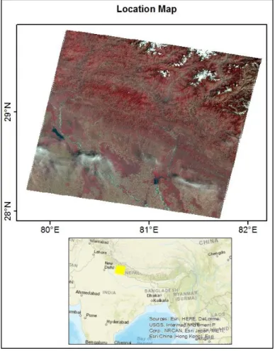
Image of the area between Nepal and India was used in the study. 148 image scene for different dates was used for the study. The figure below presents the location of the data.

Figure 4 Location of the Data

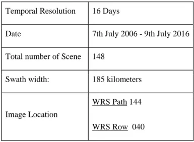
Image captured from 7th July 2006 to 9th July 2016 and having cloud cover less than 80% was used for the experiment. The specification of the image is specified in table 1.

Specification Characteristics

Spatial Resolution 30 meters

(22)

13 Temporal Resolution 16 Days

Date 7th July 2006 - 9th July 2016

Total number of Scene 148

Swath width: 185 kilometers

Image Location

WRS Path 144

WRS Row 040

Table 1 Specification of Image Used. Source: USGS

Benchmark Structure

3.3.

The experiment in SciDB was conducted in varying data size, varying number of SciDB instances and a varying number of CPU cores. The various benchmark parameters were selected to explore how the system performs with different variables. The size of data window and an actual number of cells is shown in table 2. The table also presents the size of image array and computed NDVI array in megabytes (MB) for that window. The image was stored as an unsigned 8-bit integer and NDVI was stored as a double-precision decimal. The actual number of cells is less than the value obtained by multiplying row, column and time of data windows because of missing cell values and missing scanned lines in the images. Biggest data window was about 100 times bigger than the smallest.

Row*Column*Time Actual Number of Cells

Size of NDVI array in MB

Size of Image Array in MB 300*300*148 9283527 74.3 18.6 600*600*148 38259970 306 76.5 850*900*148 83741253 669.9 167.5 1450*1450*148 243187286 1945.49 486.4 2100*2100*148 578152493 4625.2 1156.3 3000*3000*148 1165204506 9321.6 2330.4

(23)

14

Table 2 Size of Data Window

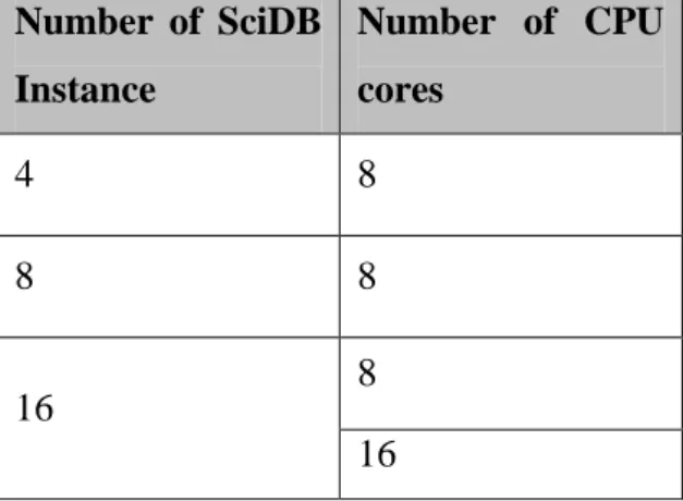
We conducted the experiment with 4, 8 and 16 number of SciDB instances running on the same physical machine. All the experiment was conducted using 8 CPU cores of the server. Furthermore, we also tested the performance by changing the number of CPU cores to 16 for 16 SciDB instances. This information is summarized in table 3.

Number of SciDB Instance Number of CPU cores 4 8 8 8 16 8 16

Table 3 Number of SciDB instances and CPU cores

Experiment in raster file with parallel support was also conducted in same data window as mentioned in table 2. This experiment was conducted using 8 CPU cores and 16 CPU cores.

All the experiments were conducted at least three times and average response time was recorded. It is the time interval between the request and the system finishes the processing and response. The time was measured using “time” command in Linux shell.

Operations

3.4.

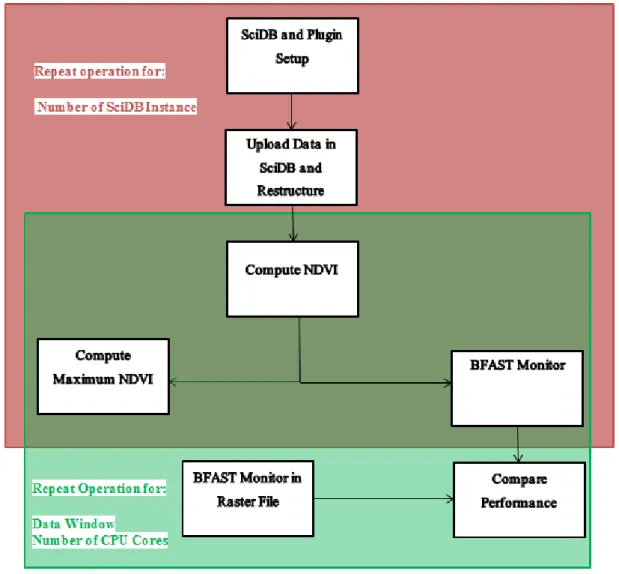
First hardware and software were set up on the server. After that, Landsat data was uploaded to the SciDB server. Then we conducted benchmark study with different parameters. We created NDVI array from our original data in SciDB. Afterward, we computed the maximum value of NDVI for each time series. Next, we also performed BFAST monitoring to detect the change from NDVI in both SciDB arrays as well as raster files. These operations were not conducted only once but repeated for different benchmark parameters. Figure 5 presents the workflow of operations. First two

(24)

15

operations were conducted once for each 4, 8 and 16 SciDB instances. NDVI computation, maximum NDVI computation and BFAST monitoring in SciDB were repeated for different data window and different numbers of CPU cores in each SciDB configuration. BFAST monitoring in raster file was also done on different data window and different numbers of CPU cores. The operations are explained in the following subsections.

Figure 5 Workflow of operations

System Setup 3.4.1.

A single server with Ubuntu Operating System was used to perform all the experiments. Detailed specification of the server is provided in appendix A.

(25)

16

SciDB and other necessary plugins were installed using docker image of SciDB. (Appel, scidb-eo, 2016). The images contain SciDB, Shim, the scidb4geo extension for space-time arrays, a GDAL driver to upload and download Earth Observation datasets and r_exec plugin. The configuration file of SciDB is in the appendix.

Shim is a web service which exposes simple API for the client to interact with SciDB through HTTP connection. Scidb4gdal and Scidb4geo plugins were installed in order to facilitate conversion between time-service imagery to the multidimensional SciDB array and SciDB array to raster. Particularly Scidb4geo plugin (reference) stores spatial and temporal reference information of the time series satellite imagery to SciDB's system catalog. Scidb4gdal is a GDAL driver implements read and write access to SciDB array. R_exec plugin was used to run R scripts inside SciDB chunks. Communication to the server was done by either by Secure Shell (SSH) protocol or using R client. The scidb package of R uses shim to connect to SciDB database and execute the query.

Loading Data to SciDB and Restructuring it 3.4.2.

The data was uploaded in SciDB using the gda_translate function of the gdalUtils library in R interface. The date of the image scene was extracted from its name and the image was placed in multidimensional array accordingly. The code to upload data is provided in appendix C.

Only two bands from the available image were loaded in SciDB separately and they were joined later to make a single array. The AFL query to join band 3 and band 4 is: store(join(LS3,LS4),LS)

Though smaller subsets of data were used for benchmark study, the whole scene was uploaded and restructured initially. The schema of data after the data upload was as follows

<band3:uint8,band4:uint8> [y=0:7023,4322,0,x=0:7857,4322,0,t=0:*,1,0]

The schema suggests array has two attributes viz. band 3 and band 4 both with data type unsigned 8-bit integer. It is a 3-dimensional array. The dimensions where x, y,

(26)

17

and t, where x and y represented horizontal coordinates while t represents time dimension. The value of y dimensions varies from 0 to 7023, x from 0 to 7857 and t starts at 0 and is unbounded. The 4322 value in the schema is the chunk size.

After that, the repart operator in AFL was used to restructure data in chunk size of 60*60*256. It means each chunk stores complete time series of 60 rows and 60 columns. To run change monitoring (Section 3.5.4) using the r_exec plugin it is necessary that each chunk contains complete time series. Thus it is necessary to set t dimension as 256 to encompass all the time series in a single chunk. It is recommended to store roughly 10 to 20 MB of data in each chunk to optimize the performance of the SciDB array (SciDB User's Guide, 2013). Considering this, the value of row and columns was selected as 60.

Also, the queries to compute NDVI (Section 3.5.2) and find maximum NDVI (Section 3.5.3) can be run in any chunk configuration. But, we conducted an experiment and found out that maximum NDVI computation is highly efficient when chunk contains all the data of time series.

Based on this appropriate chunk size was selected. AFL query to repart Image array is :

store(repart(LS,<band1:uint8,band1_2:uint8>[y=0:7023,60,0,x=0: 7857,60,0,t=0:*,257,0]),LS_repart)

The data schema looks as follows after repart operation:

<band3:uint8,band4:uint8> [y=0:7023,60,0,x=0:7857,60,0,t=0:256,1,0]

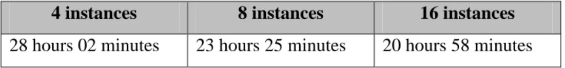
Uploading data, joining different array and changing chunk size are very time-consuming operations. The total time for this operation in different SciDB configuration is presented in table

4 instances 8 instances 16 instances

28 hours 02 minutes 23 hours 25 minutes 20 hours 58 minutes

(27)

18

After storing and restructuring data we can conduct any time series analysis on it. So this can be considered as a one-time operation. Thus we haven‟t accounted this time in computation time presented in the result section.

Normalized Difference Vegetation Index Computation 3.4.3.

Normalized difference vegetation index is the most frequently used index for vegetation studies. NDVI is calculated from the visible and near-infrared light reflected by vegetation. Chlorophyll pigment present in plant leaf absorbs a major portion of the visible spectrum of light for photosynthesis. However, it does not absorb NIR and some portion of it is transmitted and rest is reflected. This reflected NIR is captured in remote sensing and used for the study of vegetation. NDVI can be calculated as

NDVI=

NIR = Near Infra Red Radiation ; Red = Visible Red Radiation

NDVI values range from +1.0 to -1.0. Very low values of NDVI (0.1 and below) correspond to barren areas of rock, sand, or snow. Moderate values represent shrub and grassland (0.2 to 0.3), while high values indicate temperate and tropical rainforests (0.6 to 0.8).

AFL was used to subset array into the desired size, compute NDVI and store the file. NDVI was calculated for different array size and using a different number of SciDB instances. The code for the query is:

store(apply(between(landsat_array_repart,2150,2050,0,4250,4150,226),n dvi,(double(band1_2)double(band1))/(double(band1_2)+double(band1))),n dvi_windowSize)

Maximum NDVI Computation 3.4.4.

Maximum NDVI is derived from the time series NDVI array. AFL was used to subset array into the desired size, compute maximum NDVI. AFL query to compute maximum NDVI array is:

store(aggregate(between(NDVI_array,2150,2050,0,4250,4150,226),max(ndv i),x,y),ndvi_max_windowSize)

(28)

19 Change Monitoring

3.4.5.

BFAST monitor function was used to monitor change in from the time series data. This function was applied on both SciDB array and raster file. Because of too much cloud on some day, Landsat data was not available at every 16-days interval within our study period. So we have to first create regular time series objects using the bfastts function in the BFAST package. This function link data with the date information and convert data of irregular date to daily time series. The start of monitoring period was chosen as 1st Jan 2012. A season-trend model with the harmonic seasonal pattern was used as a regression modeling to detect and models the stable history. Reverse-ordered CUSUM test (ROC) was used to determine the size of the stable history period. All other default parameters were used for the processing. BFAST monitor function was run in SciDB using the r_exec plugin. The input for this operation was a SciDB array of NDVI values. R_exec works in each chunk and give the result for the chunk. For each chunk, we first split data apart. There are many options available for it, like the plyr package, data table package or tapply function in the basic package. We experimented with above three and found data table was fastest so used it. We then apply bfastmonitor function on the split data. Finally, we combined the output of the bfastmonitor function performed on split data together. The output of the operation is a 1-dimensional array with its row, column, breakpoint and magnitude value as attributes. We subsequently re-dimensioned the array into a two-dimensional array using row and column value. Iquery command to run bfastmonitor in SciDB is presented in appendix C.

BfastSpatial package in R (Dutrieux, 2016) provides a function to run BFAST monitor with parallel support and we used this package to process raster files. This function uses the mclapply function of the Parallel package in R to parallelize work in multiple processors. The code is provided in appendix C.

(29)

20

Results

Chapter 4:

This section presents the findings of the experiment conducted.

NDVI Computation

4.1.

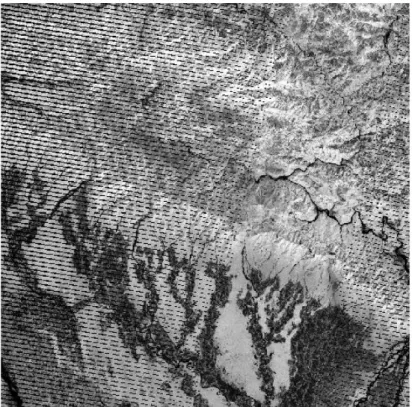
The primary output of the study was a three-dimensional array of NDVI value. NDVI not only detects vegetated area from non-vegetated but also can be used to derive vegetation health and other ecosystem dynamics. In this research, NDVI was also an input for subsequent experiments. SciDB automatically ignores cells in the array where values are missing and assign it as „NA‟.

The figure 6 shows part of NDVI array visualized in R. The strips in the image are the missing scan lines.

(30)

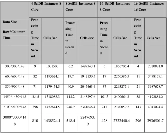
21 Data Size Row*Column* Time 4 SciDB Instances 8 Core 8 SciDB Instances 8 Core 16 SciDB Instances 8 Core 16 SciDB Instances 16 Core Proc essin g Time in Seco nd Cells /sec Proces sing Time in Secon d Cells /sec Proce ssing Time in Secon d Cells /sec Proc essin g Time in Seco nd Cells /sec 300*300*148 9 1031503 6.2 1497343.1 5 1856705.4 4 2320881.8 600*600*148 32 1195624.1 19.7 1942130.5 17 2250586.5 11 3478179.1 850*900*148 71 1179454.3 40.9 2047463.4 37 2263277.1 21 3987678.7 1450*1450*148 184.5 1318088.3 113.2 2148297.6 101.3 2400664.2 58 4192884.2 2100*2100*148 398 1452644.5 246.9 2341646.4 211 2740059.2 143 4043024.4 3000*3000*14 8 810 1438524.1 518.4 2247693. 9 428 2722440.4 296 3936501.7

(31)

22

Figure 7 Cells processed per second for NDVI computation

Table 5 presents the processing time to compute NDVI by using a different number of instances and CPU cores for the different subsets of the array chosen for testing. We also normalized values to a common time basis to provide a speed metric. I.e. we computed cells processed per second. The graph in figure 7 plots number of cells processed in unit second against data size. The data in the x-axis is plotted in log scale to incorporate a large range of value in this graph.

It is very vivid in the graph that the performance of the system increases when we increase the number of instances from 4 to 8 and then to 16. However, we can also notice that incremental benefit of increasing number of instances to the cluster decrease with added instances.

Another interesting thing to note from the metrics data is when we increased the cores available for SciDB container from 8 to 16 the system is able to incorporate it in the computation. The system speeds up by the median value of 1.5 when we used 16 instances with 8 cores to 16 instances with 16 cores.

We can also see that performance of the computation also varies with data size. Generally, increasing data sized showed an increase in performance until some saturation point with some variations.

0.0E+00 5.0E+05 1.0E+06 1.5E+06 2.0E+06 2.5E+06 3.0E+06 3.5E+06 4.0E+06 4.5E+06 8 32 128 512 2048 Cel l/Sec

Data Size (Cell counts in Millions)

16 SciDB Instances 16 Core

8 SciDB Instances 8 Core 4 SciDB Instances 8 Core

(32)

23

Maximum NDVI Computation

4.2.

Finding the maximum value of NDVI at a particular location is the simplest form of time series analysis yet very useful to summarize the time series. It is also an input for other analysis such as to compute Vegetation Condition Index (VCI). This time series analysis gives a 2-dimensional array of maximum NDVI value observed over the chosen time period. This 2-dimensional array visualized using R is presented in figure 8. In this image, there are no strips of missing scanned line as seen in NDVI image because missing lines do not overlap in all image and are removed while taking maximum value.

(33)

24 Data Size Row*Colum n*Time 4 SciDB Instances 8 Core 8 SciDB Instances 8

Core 16 SciDB Instances 8 Core 16 SciDB Instances 16 Core Proce ssing Time in Secon d Time Series /sec Proce ssing Time in Secon d Time Series /sec Proces sing Time in Secon d Time Series /sec Processin g Time in Second Time Series /sec 300*300* 148 1.7 53294.71 1.1 82364.55 1 90601 0.8 113251.3 600*600* 148 5.1 70823.73 2.51 143904.8 2.12 170377.8 1.5 240800.7 850*900* 148 10.3 74441.84 5.4 141990.9 4.4 174261.6 2.75 278818.5 1450*1450 *148 17.4 121000.1 13.8 152565.3 11.2 187982.2 7.6 277026.4 2100*2100 *148 42 105100 28.6 154342.7 23.6 187042.4 15 294280.1 3000*3000 *148 90 100066.7 60 150100 49 183795.9 31.4 286815.3

(34)

25

Figure 9 Time series processed per second for maximum NDVI computation

The table 6 and figure 9 present the performance of SciDB for maximum NDVI benchmark. Table 6 shows response time for different data size and a varied number of SciDB instances and CPU cores. The x-axis in figure 10 is data size represented by the number of cells. It is plotted in log scale. Y-axis shows the number of time series processed per second obtained by normalizing computation time with the total number of time series. The result shows similar characteristic with that of computing NDVI. However, the time taken for computation varies from a fraction of seconds to few minutes. From the graph, it can be observed that the influence of an increase in the number of instances and cores is lesser for smallest data. We can also see slightly better performance for third data window for 4 SciDB instances.

Change Monitoring

4.3.

Analysis to detect changes in SciDB array and in Raster file with multicore parallelization was performed using bfastmonitor function. Bfastmonitor monitors change in time series by detecting disturbances in the end of time series. The output for this analysis was raster while processing raster file and array in case of SciDB with two values: the breakpoint detected with the date when this breakpoint is

0 50000 100000 150000 200000 250000 300000 350000 8 32 128 512 2048 Ti m e ser ies/Sec

16 SciDB Instances 16 Core 16 SciDB Instances 8 Core 8 SciDB Instances 8 Core 4 SciDB Instances 8 Core

(35)

26

detected and magnitude of the median difference between the observed value and the value predicted by in the monitoring period. All the cells are assigned a value for magnitude regardless of whether the change is detected or not but no breakpoint date is assigned for the cells for which breakpoint is not detected.

Since the parameters used, preprocessing done and resampling method selected was similar, the output (cell values) of applying bfastmonitor in raster file was similar to the output of same analysis in SciDB. The figure below presents the output of this experiment.

(36)

27

Figure 11 Breakpoint detected by BFAST Monitor with year

The red area in figure 10 represents the area where change magnitude is higher and green area of the figure suggest lower change magnitude. Figure 11 shows the location of breakpoint detected with the year in which breakpoint is detected. It is important to note that all these changes might not be due to an actual change in the ground, which could be due to noise such as cloud in data of monitoring period. So further post processing is necessary but that is not the scope of our study.

The following two subsections describe the performance measured for running this experiment in SciDB and file system with parallel support.

In SciDB 4.3.1.

This experiment gives result in a 1-dimensional array with change value which was subsequently into a two-dimensional array with x and y dimension. The time to redimension the array was far less compared to the time to run bfastmonitor, and for this benchmark study, we did not consider the time to redimension the array. Time to repart array (change chunk size) is also not included in the time presented in the result.

(37)

28

Table 7 presents time taken to run bfastmonitor for different experiment conditions. To get a better insight into the performance we also computed time series processed per second for all experiment conditions. The graph in figure 12 plots number of time series processed per second against different data window. A log scale is used in x-axis to show the large range of value in our graph without smaller values being compressed at the left of the graph.

The graph is not different than graph obtained in previous benchmarks. However, time elapsed to during this computation ranges from around few minutes to more than 21 hours.

The performance of the system increases for all data size when the number of SciDB instances is changed from 4 to 8 and then 8 to 16. Though the rate at which the system scale up decreases with increasing number of instances. When the CPU core of the system is increased from 8 to 16 for 16 SciDB instances the performance increase significantly for all array subsets.

In this experiment also the performance of the system varies slightly with the data size. Data Size Row*Colum n*Time 4 SciDB Instances 8 Core 8 SciDB Instances 8 Core 16 SciDB Instances 8 Core 16 SciDB Instances 16 Core Processin g Time in Second Time Series /sec Processi ng Time in Second Time Series /sec Process ing Time in Second Time Series /sec Processin g Time in Second Time Series /sec 300*300*1 48 847 107 584 155.1 562 161.2 403 224.8 600*600*1 48 3285 110 2026 178.3 1874 192.7 1184 305.1

(38)

29 850*900*1 48 6643 115.4 4277 179.3 3821 200.7 2200 348.5 1450*1450 *148 18141 116.1 11154 188.8 10446 201.6 5831 361.1 2100*2100 *148 37593 117.4 24165 182.7 21285 207.4 12403 355.9 3000*3000 *148 76438 117.8 49948 180.3 44870 200.7 25290.5 356.1

Table 7 Performance Metrics for BFAST monitoring function in SciDB

Figure 12 Time series processed per second for BFAST monitor query in SciDB

In Raster file with parallel support 4.3.2.

BFAST monitor with parallel support was run using 8 and 16 CPU cores. The result is tabulated below. 10 60 110 160 210 260 310 360 410 8 32 128 512 2048 Ti m e Ser ie s p ro ce ssed / sec

(39)

30

Figure 13 shows the bar graph of time series processed per second using 8 cores and 16 cores. To compare the performance with SciDB we have also plotted the performance of SciDB with 8 core and 8 instances and SciDB with 16 core and 16 instances.

Data Size Row*Column*Time

R Parallel with 8 core R Parallel with 16 core Processing Time In Seconds Time series per sec Processing Time In Seconds Time series per sec 300*300*148 617 146.8 559 162.1 600*600*148 2130 169.6 1900 190.1 850*900*148 5483 139.8 4042 189.7 1450*1450*148 12089 144 10928 192.7 2100*2100*148 26728 165.2 24150 182.8 3000*3000*148 68099 132.2 45548 197.7

(40)

31

Figure 13 Comparison of processing time in raster file and SciDB array

It is clear from above graph that SciDB performs better than running BFAST monitor in raster file with multi-core parallelization. We can also notice that difference of performance is higher for 16 core processor than 8 core processor.

To better understand this incremental performance we computed speed up obtained by using SciDB in 8 core machine and 16 core machines. Here speedup is the ratio of the processing time of raster file to SciDB array. Speed up in a different number of CPU cores is presented in table 8 and also plotted in figure 14.

Data Size

Row*Column*Time

Speed up of SciDB over File system 8 Core Processor 16 Core Processor

300*300*148 1.06 1.39 600*600*148 1.05 1.6 850*900*148 1.28 1.84 1450*1450*148 1.31 1.87 2100*2100*148 1.11 1.95 3000*3000*148 1.36 1.8

Table 9 Metrics of Speed up of SciDB over File system

0 50 100 150 200 250 300 350 400 Ti m e Ser ie s/Sec o n d Data Window

File Processing with 8 core

File Processing with 16 core

(41)

32

Figure 14 Speed up of SciDB over file system

From the figure, we can see that processing in SciDB Array is faster than file-based processing for all data size in both 8 core machine and 16 core machine. But the Speedup is not significant in 8 core machine and it is up to 1.3. However, the speedup in 16 core machine is substantial with the value up to 1.95.

0 0.5 1 1.5 2 2.5 300*300*148 600*600*148 850*900*148 1450*1450*148 2100*2100*148 3000*3000*148 16 Core Processor 8 Core Processor

(42)

33

Discussion

Chapter 5:

Discussions of the Study

5.1.

This study shows qualitatively how multitemporal images can be managed and analyzed in SciDB and quantitatively performance to run such query.

We demonstrated storage of multitemporal image as SciDB array and approach for indices computation and simple and complex time series analysis on SciDB array. We observed that product obtained by running process in the file system and in SciDB were exactly identical. This was expected because we selected similar parameters for processing and did similar preprocessing.

Benchmark Study 5.1.1.

Regarding the benchmark testing, the graph of performance for three analysis done in the SciDB arrays is rather similar, though the order of response time is different. Computing NDVI and maximum NDVI took up to few minutes while change monitoring took hours. The reason for this is the different complexity of computation. Ideally, the number of cells processed per second or number of time series processed per second should be same irrespective of the data size. But we can see the variation in performance for different data window. The reason can be found by understanding the storage and computation architecture of SciDB.

The data in SciDB is partitioned and stored in chunks of predefined size. These chunks are stored and processed in different SciDB instances and one instance cannot share processing with other SciDB instance. Hence due to unequal distribution of chunk across SciDB instances in the different data window, we can see the variation in performance for different data size. Another factor contributing to that is uneven cell density within the chunks. Because of missing cells and missing scanned lines in Landsat image, a number of cells in each chunk is different, this uneven distribution of workload in different chunks also contribute to the variation in performance. The variation is higher for smaller array size when 8 or 16 SciDB instances were used. The reason for this is in our experiment smaller data cannot make use of all

(43)

34

added instances. For example, the smallest data was stored in 5 chunks. So when the number of instances increased from 4 to 8 it could not make the use of additional 3 instances. Variation is lesser for bigger data because the difference in the amount of data in different instances is small relative to whole data. Therefore, all the SciDB instances can contribute more or less equally for the computation. Still, optimal performance is obtained when we consider data size and available instances in addition to recommended volume of data(10MB to 20MB) when selecting chunk size. All the processes showed an increase in performance when the numbers of instances were increased for all data size. This justifies SciDB‟s ability to run the process in parallel in different instances. However, increasing the number of the instance from 8 to 16 does not increase the performance in the same rate as it was increased when we changed the number of SciDB instances from 4 to 8. This is not surprising because when we increase the number of the instance without increasing processing resource, the additional instance has to share the same processing resource and the relative contribution of each additional instances get smaller.

However, when we increase the number of processors, the performance of the system increases significantly. For instance, running BFAST monitor operation in 16 SciDB instances in 16 core machine is about 1.7 times faster than running with 16 SciDB instances in 8 core machine and about 1.9 faster than running with 8 SciDB instances in 8 core machine. This suggests that SciDB scales out with additional SciDB instances. But it is also important to consider that the computing resources available for SciDB are adequate. This computing resource can be provided either by increasing computing capacity of the machine or adding new SciDB instances to a new machine connected by a network. When storage and computation requirement of the system increases with the increasing amount of imagery, SciDB system can still be used by adding more SciDB instances either on the same server by increasing its storage and computing capacity or in other machines in the grid.

(44)

35

Comparison of SciDB and file-based Processing 5.1.2.

The major differences found between SciDB based solution and file-based solution for multitemporal images are summarized in points below

Time and effort for Data Preparation: It can be seen that there are few time-consuming steps in SciDB before the data can be actually processed. Data has to be uploaded to the database and it should be restructured for processing. So SciDB might not be a better solution when data size is tiny. The intermediate steps not only increases total computation time but also the complexity of the solution.

Speed: From a comparison of SciDB with multi-core processor based parallelization of time series, it is apparent that SciDB performs better for all data size if we do not consider the time to upload data and restructure it. Serial operations at the beginning and end of the process can partly explain the higher processing time in multi-core processor based parallelization. It is also found that this Speedup of SciDB over file system is further increasing with increasing number of processors. So when the data size is very big so is the computing resources, the difference in processing time between using file system and using SciDB will be highly magnified.

Ease of data management: Data management operations are easier in the case of SciDB then in raster file. In file system, date and other metadata have to be stored in the file name. Thus searching of metadata is challenging while it is quite easy in the database. In SciDB it is easier to select Multidimensional window and retrieve or subset the array and save as a new array based on requirement. However, it is more difficult to crop and retrieve required data from raster stack.

Ease of computation: SciDB is not a matured system and there are very few documents and manuals and user community is also smaller. Library of SciDB is basic and limited. Further SciDB does not have good support for remote sensing operations. Running analysis using r_exec was also not straightforward. The function can take only specific input and give some specific output. There was not any document that describes how the function works. Further, debugging is very difficult while running script using r_exec.

(45)

36

Scalability: The most important distinction is SciDB‟s ability to provide horizontal scalability. SciDB instances can be installed in distributed machine within a cluster. So data can be stored in different nodes and can be processed there. Thus SciDB can be scaled out to any big data. On the contrary, multicore-based processing provides vertical scaling. That is we can scale by adding more CPU and memory to an existing machine. This scaling is often limited by the capacity of a single machine. This system might not work when the very big data size and extremely high computational requirements. Thus in the case of really big Remote sensing data file based processing (Using multicore parallelization) might not be applicable but SciDB has potential to provide the solution for any big RS data.

Limitations of the Study

5.2.

The study has following limitations:

1. Because of the limitation of time and resource, the data size used in the study has a moderate size and cannot be considered really big RS data. Though some of the computations were not possible to run using the serial code and some query took more than 21 hours to complete in our system even with parallel processing. However, the image size was less than 40 gigabyte and it is very tiny portion compared to all the available image of Landsat. Nevertheless, we discussed how SciDB can be scaled out to a number of distributed servers in case of really big RS data.

2. We performed the experiment only for simple arithmetic computation and time series analysis in this study. Similarly, the methodology can also be applied for other analysis like clustering. The major difference will be the different storage schema in the chunks. However further study is needed to run some of the analysis which needs user interactions.

3. Experiments were conducted in a single server cluster and not in multiple machines. Actually, multi-core based processing is possible only on a single server, whereas SciDB instances can be installed either on distributed machine or same server as long as computational and storage resource is sufficient.

(46)

37

4. The speed of query in SciDB also depends on in the function used within the r_exec. The query can also be optimized using less for loops and fewer condition checks.

(47)

38

Conclusion and Future Work

Chapter 6:

System having distributed storage and horizontal scalability is the solution to ever increasing need of storage and computational requirement of remote sensing big data. In this experiment, we demonstrated a scalable solution for the management and the processing of multitemporal satellite imagery using SciDB.

Analysis of multitemporal imagery was run in parallel, in more than one SciDB instances, in this study. We found out that the performance of the system increase when the number of SciDB instance increases provided that there is enough computational resource (processor) for the added instance.

It is also important to better understand SciDB architecture for optimal performance. It is essential to select an appropriate number of chunk size based on our data window and number of SciDB instances for better performance. Chunk shape and size also depends on the type of analysis we are performing inside SciDB.

SciDB provides faster and flexible solution compared to multicore-based parallel processing of raster file for multitemporal images. The multi-core based parallelization cannot meet the high computational requirements in many remote sensing applications.

However, it is important to mention that SciDB might not be the best solution for analyzing small data. Also, relative immaturity of SciDB and limited in-built support of remote sensing increase the complexity for the scientist to develop SciDB based solution.

Nevertheless, it can be concluded from the study that SciDB provides the high performance scalable solution for management and time series analysis of the multitemporal image and it has the potential to meet the ever increasing storage, management and computational need of big remote sensing data.

Further research can be conducted in the same research direction. In this study, we demonstrated the use of SciDB for time series analysis of satellite imagery. We also discussed how it can be applied for analysis like clustering. However, it is necessary

(48)

39

to investigate further for applications which require more user interactions such as Supervised Classification. Similarly distributed processing framework like Hadoop, Google MapReduce can also be used for processing of Big RS data. Comparing this with SciDB in terms of ease of data management and speed of processing can also be useful to direct the future of HPC. Another interesting area of study is the use of SciDB as the backend for web-based image processing system. The Web allows the wider user community to access remote sensing resource and SciDB can act as a tool to manage and process such data.

(49)

40

Bibliography

Chapter 7:

Anyamba, A., & Eastman, J. (1996). Interannual variability of NDVI over Africa and its relation to El Niño/Southern Oscillation. International Journal of Remote Sensing. 1;17(13), 2533-2548.

Appel, M. (2016). scidb-eo. Retrieved from github: https://github.com/appelmar/scidb-eo

Appel, M., & Pebesma, E. (2016, May 11). Scalable Earth Observation analytics with R and SciDB. Retrieved September 2016, from r-spatial:

http://r-spatial.org/r/2016/05/11/scalable-earth-observation-analytics.html

Clark, M. L., Aide, T. M., Grau, H. R., & Riner, G. (2010). A scalable approach to mapping annual land cover at 250 m using MODIS time series data: A case study in the Dry Chaco ecoregion of South America. Remote Sensing of Environment, 114(11), 2816-2832.

Crist, E. P., & Cicone, R. C. (1984). A Physically-Based Transformation of Thematic Mapper Data-The TM Tasseled Cap. IEEE Transactions on Geoscience and Remote Sensing , 22(3), 256− 263.

Cudre-Mauroux, P., Kimura, H., Lim, K.-T., Rogers, J., Madden, S., Stonebraker, M., et al. (2010). SS-DB: A Standard Science DBMS Benchmark. Retrieved

October 2016, from

http://www-conf.slac.stanford.edu/xldb10/docs/ssdb_benchmark.pdf Dutrieux, L. (2016). bfastSpatial. Retrieved from github:

https://github.com/loicdtx/bfastSpatial

Eddelbuettel, D. (2017). High-Performance and Parallel Computing with R. Retrieved from CRAN:

(50)

41

Hausen, E. (2016). Array-database Model (SciDB) for Standardized Storing of Hyperspectral Satellite Images. Master Thesis.

Jacobs, A. (2009). The pathologies of big data. Communications of the ACM, 52(8), 36-44.

Kambatla, K., Kollias, G., Kumar, V., & Grama, A. (2014). Trends in big data analytics. Journal of Parallel and Distributed Computing, 74(7).

Karantzalos, K., Bliziotis, D., & Karmas, A. (2015). A Scalable Geospatial Web Service for Near Real-Time, High-Resolution Land Cover Mapping. Selected Topics in Applied Earth Observations and Remote Sensing, IEEE Journal of,Volume: 8, I, 4665 - 4674 .

Kitchin, R. (2014). Big Data, new epistemologies and paradigm shifts. Big Data & Society, 1(1).

Laney, D. (2001). 3D Data Management: Controlling Data Volume, Velocity, and Variety. Retrieved from

http://blogs.gartner.com/doug- laney/files/2012/01/ad949-3D-Data-Management-Controlling-Data-Volume-Velocity-and-Variety.pdf

Lee, C., Gasster, S. D., Plaza, A., Chang, C.-I., & Huang, B. (2011). Recent

developments in high performance computing for remote sensing: A review. IEEE Journal of Selected Topics in Applied Earth Observations and Remote Sensing, 4(3), 508-527.

Leutner, B., & Horning, N. (2017, 01 10). RStoolbox: Tools for Remote Sensing Data Analysis. Retrieved from CRAN:

https://cran.r-project.org/web/packages/RStoolbox/index.html

Lewis, B. W. (2016). Run R programs within SciDB queries. Retrieved from https://github.com/Paradigm4/r_exec

Li, S., Dragicevic, S., Castro, F. A., Sester, M., Winter, S., Coltekin, A., et al. (2016). Geospatial big data handling theory and methods: A review and research

Scalable analysis of multitemporal images using an array database

Scalable Analysis of Multitemporal Images Using an Array

Database

Abhasha Joshi

Scalable Analysis of Multitemporal Images Using an

Array Database

Declaration

Acknowledgements

Abstract

Keywords

Table of Contents

List of Figures

List of Tables

Introduction

Chapter 1:

Background and Motivation

1.1.

Aims and Objectives

1.2.

Thesis

Organization/ Structure

1.3.

Literature Review

Chapter 2:

Big Earth Observation Data

2.1.

High Performance Computing in RS

2.2.

R for HPC in Remote Sensing

2.3.

SciDB

2.4.

Time Series Analysis

2.5.

Methodology

Chapter 3:

Design Consideration

3.1.

Data Used

3.2.

Benchmark Structure

3.3.

Operations

3.4.

Results

Chapter 4:

NDVI Computation

4.1.

Maximum NDVI Computation

4.2.

Change Monitoring

4.3.

Discussion

Chapter 5:

Discussions of the Study

5.1.

Limitations of the Study

5.2.

Conclusion and Future Work

Chapter 6:

Bibliography

Chapter 7: