Júri
Presidente: Prof. Doutora Maria da Ascensão M. Reis Arguentes: Prof. Doutor Olivier Gonçalves
Prof. Doutor João A. Lopes Vogais: Doutor Luis da Costa
Doutora Cláudia Galinha Loureiro
Marta Filipa Batista de Sá
Mestre em Engenharia Alimentar
Dezembro, 2019
Monitoring of biological processes in microalgae
production using Fluorescence Spectroscopy
Dissertação para obtenção do Grau de Doutor em
Engenharia Química e Bioquímica – Especialidade Engenharia Bioquímica
Orientadora: Cláudia Galinha Loureiro
Investigadora
Faculdade de Ciências e Tecnologia - Universidade Nova de Lisboa
Co-orientadores: João Goulão Crespo
Professor Catedrático
Faculdade de Ciências e Tecnologia - Universidade Nova de Lisboa
Maria Barbosa
Professora Catedrática
iii Monitoring of biological processes in microalgae production using Fluorescence Spectroscopy
Copyright © Marta Filipa Batista de Sá, Faculdade de Ciências e Tecnologia, Universidade Nova de Lisboa.
A Faculdade de Ciências e Tecnologia e a Universidade Nova de Lisboa têm o direito, perpétuo e sem limites geográficos, de arquivar e publicar esta dissertação através de exemplares impressos reproduzidos em papel ou de forma digital, ou por qualquer outro meio conhecido ou que venha a ser inventado, e de a divulgar através de repositórios científicos e de admitir a sua cópia e distribuição com objectivos educacionais ou de investigação, não comerciais, desde que seja dado crédito ao autor e editor.
v “(…) It matters not how strait the gate, How charged with punishments the scroll, I am the master of my fate, I am the captain of my soul.”
Invictus in Book of Verses, William Ernest Henley (1888).
vii
Acknowledgements
O doutoramento foi uma etapa na minha vida que contribuiu para o meu crescimento profissional e pessoal. São anos de muito trabalho e dedicação, altos e baixos, mas o que se recorda são as conquistas e alegrias e o sentimento de realização. Este percurso teria sido insuportável sem o apoio de diversas pessoas às quais gostaria de expressar o meu profundo agradecimento.
Antes de mais, gostaria de agradecer aos meus orientadores Cláudia Galinha e João Crespo, por terem acreditado em mim e me terem dado a oportunidade de realizar este trabalho. Mas sobretudo, ficarei para sempre grata por me terem dado a liberdade que precisei para crescer como investigadora, para seguir as minhas ideias e traçar o percurso do meu doutoramento. Gostaria de agradecer ao João pela oportunidade que me proporcionou de participar em conferências e pelo incentivo de fazer um estágio no estrangeiro. Cláudia, espero que, como primeira aluna, não tenha sido muito difícil de aturar! Muito obrigada por estares sempre disponível para mim, obrigada pelo apoio e por teres sempre uma palavra amiga.
À minha orientadora Maria Barbosa, faltam-me as palavras para expressar o quão grata estou por me ter acolhido! Obrigada pelo voto de confiança, por acreditares em mim, pelo carinho e preocupação com o meu bem-estar. És uma enorme inspiração para qualquer mulher na ciência, e estou extremamente grata pela aprendizagem e experiência que adquiri por trabalhar lado-a-lado contigo.
Um agradecimento a todos os colaboradores da A4F – Algae for Future, em especial ao Dr. Luís Costa, à Celina Parreira, ao Pedro Fonseca e à Joana Galante, pela partilha de conhecimentos e boa disposição com que sempre me receberam.
Aos meus colegas do BPEG agradeço a boa disposição, entreajuda e oportunidade de partilhar bons momentos. Ao longo destes anos várias pessoas passaram pelo grupo que deixaram um carinho muito especial. Um muito obrigado pela boa disposição e companheirismo, à Catarina Oliveira, ao Christophe Roca, à Carla Daniel e à Joana Cassidy.
Luísa Neves, obrigada pelo apoio incondicional que me deste nas fases mais difíceis destes últimos anos. Obrigada por estares sempre disposta a ouvir, pelo teu ombro amigo, pelos teus conselhos. Mónica Carvalheira, obrigada por estares sempre disponível para me ajudares no que fosse preciso. Nunca esquecerei as nossas infindáveis conversas no infernal trânsito de Lisboa! Bruno Oliveira, Tiago Costa e Eliana Guarda (tuxinha!) obrigada pela vossa boa disposição. Meus queridos, vocês têm uma energia positiva incrível. Partilhar laboratório convosco é uma alegria, mas ainda melhor é poder fazer parte das vossas vidas e ver-vos “crescer”!
Rita Ferreira, muito obrigada por tudo! Em ti encontrei uma verdadeira amiga, para os maus momentos, mas sobretudo para os momentos espetaculares. Obrigada pela tua amizade, pelo exemplo de mulher forte e independente que és!
Ricardo Marques, recordo tantos momentos que passámos juntos. Contigo partilhei caminhadas, campismos, cervejinhas ao fim do dia… festejámos santos populares, passagens de ano, festivais de verão... contigo partilhei frustrações, indecisões, profissionais e pessoais, e
viii tantas alegrias! Irei recordar-te para sempre, pelas tuas teorias malucas, mas sobretudo pela tua enorme amizade. Muito obrigada amigo!
In Wageningen I found a second home and I would like to thank all my friends and colleagues for make me feel so welcome. Special thanks to my “work-husband” Narcis Ledo, for all the knowledge you shared with me and the immense patience; to Robin Barten for all the fun moments and conversations, even when you called me old!; to Pieter Oostlander, for listening to my worries, for the amazing company in our road trip in Scotland, for all the amazing gaming nights; to Barbara Guimarães, pela tua alegria contagiante, pelos teus abracinhos! To Snezana Gegic and Fred van den End, the best technicians a PhD student could ask for! Thank you for your big patience and giant humour.
Iago Teles, obrigada por me aturares, especialmente na fase intensa de escrita. É bom ter alguém com quem posso rir e brincar e resmungar, de porta fechada e em português! Obrigada pela tua boa disposição, e por partilhares comigo as expressões de sabedoria da tua vovó!
A very warm thanks to Wendy Evers and Jorijn Janssen, who helped me so much in so many moments. It’s amazing to know that I can always count on you, girls! Thank you both for the immense support during my stay in WUR, not only in the lab but also in the coffee corner! Your joy and company always lighten up my days!
Marek Wazynski, with you we stablish our home in this foreign country. With your help and support, every challenge it’s easier to endure. Thank you for brightening my every day, thank for your love.
Às minhas amigas do peito, Erica Cabral, Alzira Ramos e Isabel Rosa, que me acompanham nesta jornada há tantos anos! Não importa em que parte do mundo nos encontremos, o grupo “Rocking the 30s” é a melhor coisa de sempre… O grupo com os temas mais loucos e variados, de alguma sabedoria, às vezes todos em simultâneo! Adoro-vos! Sem vocês, esta etapa da minha vida teria sido muito mais aborrecida e pesada. Obrigada!
Aos meus meninos de Leiria, Tiago Gonçalves, João Órfão e Ana Ramos, obrigada por fazerem parte da minha vida desde os tempos de liceu! Obrigada pelos cafezinhos na praça e pelas conversas animadas. Ao Tiago Mora, não há palavras para descrever o quanto agradeço o teu apoio incondicional. Obrigada por teres estado sempre do meu lado, nos bons e nos maus momentos.
E por fim à minha família, sobretudo ao meu mano e à minha mãe. Obrigada mãezinha por seres o meu porto de abrigo, obrigada pelo teu apoio incondicional em todas as decisões da minha vida, obrigada por tudo o que fizeste por mim, para que eu tivesse todas as oportunidades possíveis. Amo-vos muito.
ix
Abstract
Microalgae industrial production is nowadays viewed as a solution for environmental conscious and sustainable alternative production of fuel, feed, food and chemicals. Throughout the years, several technological advances have been studied and implemented that increased the competitiveness of microalgae production. However, online monitoring and a real-time process control of a microalgae production factory still requires development to support economic sustainability.
In this work, fluorescence spectroscopy coupled with chemometric modelling is studied as an online monitoring tool to be used in microalgae production. Fluorescence spectroscopy is a non-invasive and highly sensitive technique, able to detect instantaneously several natural fluorophores but also the interferences between them and the environmental media. Chemometric methods are often used to deconvolute the information within the fluorescence matrices, known as excitation-emission matrices (EMMs), and to determine the relationship between them and the parameters to be monitored.
To prove the potential of fluorescence spectroscopy coupled with chemometric modelling techniques, different strategies are studied. Firstly, the EEMs of the spectra are used as raw data, without pre-treatment for removal of water scatter and inner-filter effects. Principal Component Analysis (PCA) is used to extract the meaningful information from the spectra, resulting in Principal Components (PCs). Through Projection to Latent Structures (PLS) modelling, prediction models are developed using the PCs from the fluorescence EEMs as inputs, to find linear correlations with the parameters to be monitored, the outputs. A second strategy is studied with pre-treated EEMs. With these EEMs, two input strategies in the PLS models are tested: using directly the EEMs in PLS or compressing the EEMs into PCs though PCA prior to PLS.
Two marine microalgae are used in these studies, Dunaliella salina and Nannochloropsis oceanica. Five parameters are monitored – cell concentration, cell viability, pigments concentration, fatty acids composition and nitrogen concentration – in four different processes – cultivation, product formation (carotenoids and lipids), harvesting by membrane filtration and permeate recover.
The combination of fluorescence spectroscopy, with its high sensitivity and resolution, coupled with chemometric analysis for data pre-treatment and development of prediction models, enhances the knowledge and the possibility for real-time process control in microalgae production systems.
Keywords: online monitoring, fluorescence spectroscopy, Principal Component Analysis, Projection to Latent Structures, microalgae production, Dunaliella salina, Nannochloropsis oceanica.
xi
Resumo
A produção industrial de microalgas é atualmente vista como uma solução para a produção ambientalmente responsável e sustentável nas áreas dos combustíveis, alimentação humana e animal, e na produção de diversos compostos químicos. Ao longo dos anos, foram estudados e implementados vários avanços tecnológicos que permitiram aumentar a competitividade da produção de microalgas. No entanto, ainda é necessário algum desenvolvimento na monitorização in situ e em tempo real de forma a assegurar um controlo mais preciso da produção de microalgas e a sua sustentabilidade económica.
Nesta tese é estudada uma ferramenta de monitorização em tempo real para a produção de microalgas, tendo por base a espectroscopia de fluorescência acoplada a quimiometria. A espectroscopia de fluorescência é uma técnica não invasiva, com grande sensibilidade de deteção e especificidade. Permite detetar instantaneamente vários fluoróforos naturais, assim como as interferências entre eles e o meio de cultura. Frequentemente são usados métodos de quimiometria para extrair e deconvoluir a informação contida nas matrizes de fluorescência, conhecidas como matrizes de excitação-emissão (“excitation-emission matrices”, EEMs), e estabelecer a relação entre elas e os parâmetros a monitorizar.
Foram estudadas várias estratégias para demonstrar o potencial da espectroscopia de fluorescência acoplada a métodos quimiométricos. Em primeiro lugar, as EEMs foram usadas em bruto, sem pré-tratamento para a remoção do efeito de dispersão da radiação no meio contínuo (água) e do efeito de ”filtro interno” no meio de cultura (“inner filter effect”). Análise de componentes principais (“Principal Component Analysis”, PCA) é então usada para extrair informação das matrizes, resultando em componentes principais (“Principal Components”, PCs). Por fim, foram desenvolvidos modelos de previsão usando as variáveis observadas como informação fornecida (“inputs”) (os PCs das EEMs da fluorescência) através de projeção de estruturas latentes (“Projection to Latent Structures”, PLS), para encontrar correlações lineares com os parâmetros a monitorizar (“outputs”). Foi estudada uma segunda estratégia com o uso de EEMs pré-tratados, ou seja, sem efeito de dispersão da água e de filtro interno. Com estes EEMs pré-tratados, foram estudadas duas estratégias de fornecimento de informação (“inputs”) nos modelos PLS: usando os EEMs directamente no PLS ou depois de serem compactados em PCs através de PCA antes do PLS.
Nesta tese foram estudadas duas microalgas marinhas, Dunaliella salina e Nannochloropsis oceanica. Foram monitorizados cinco parâmetros – concentração celular, viabilidade celular, concentração de pigmentos, composição em ácidos gordos e concentração de azoto – em quatro processos diferentes – cultivo, formação do produto (carotenoides ou lípidos), colheita por filtração através de membranas e recolha de permeado.
A combinação de espectroscopia de fluorescência, de alta sensibilidade e resolução, associada à quimiometria para o pré-tratamento e desenvolvimento de modelos de previsão, aumenta o conhecimento e a possibilidade de controle em tempo real de processos na produção de microalgas.
xii Palavras-chave: monitorização em tempo real, espectroscopia de fluorescência, Análise de componentes principais, projecção de estruturas latentes, produção de microalgas, Dunaliella salina, Nannochloropsis oceanica.
xiii
Contents
ACKNOWLEDGEMENTS ... VII ABSTRACT ... IX RESUMO ... XI LIST OF FIGURES ... XVII LIST OF TABLES ... XXI LIST OF ACRONYMS... XXIII
I. INTRODUCTION... 1
I.1. Challenges in monitoring biological systems ... 1
I.2. Optical sensors - Techniques available... 2
I.2.1. Infrared spectroscopy ... 2
I.2.2. Raman spectroscopy ... 3
I.2.3. Fluorescence spectroscopy: principles ... 3
I.2.4. Fluorescence spectroscopy: biochemical applications ... 4
I.3. Chemometrics: mathematical treatment of the spectra information ... 5
I.4. Case study: microalgae production and added-value products formation ... 7
I.5. Thesis motivation and outline ... 9
I.5.1. Motivation ... 9
I.5.2. Thesis outline ... 10
II. 2D FLUORESCENCE SPECTROSCOPY FOR MONITORING DUNALIELLA SALINA CONCENTRATION AND INTEGRITY DURING MEMBRANE HARVESTING ... 13
Abstract ... 13
II.1. Introduction ... 14
II.2. Material and Methods ... 15
II.2.1. Growth conditions of green and orange Dunaliella salina ... 15
II.2.2. Membrane harvest equipment and operation conditions ... 15
II.2.3. Sampling procedure and analysis ... 16
II.2.4. Development of PCA and PLS models ... 16
II.3. Results and discussion ... 18
xiv
II.3.2. Validation with bioreactors: experiments with green Dunaliella salina culture ... 24
II.4. Conclusions ... 25
II.5. Acknowledgements ... 26
III. DEVELOPMENT OF A MONITORING TOOL BASED ON FLUORESCENCE AND CLIMATIC DATA FOR PIGMENTS PROFILE ESTIMATION IN DUNALIELLA SALINA... 27
Abstract ... 27
III.1. Introduction ... 28
III.2. Material and Methods ... 29
III.2.1. Dunaliella salina growth and carotene induction conditions ... 29
III.2.2. Sampling procedure and analysis ... 29
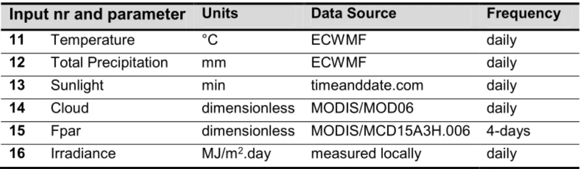
III.2.3. Climatic data ... 30
III.2.4. Development of multivariate models ... 32
III.3. Results and Discussion ... 33
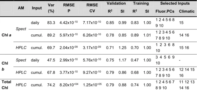
III.3.1. Chlorophylls ... 34
III.3.2. Carotenoids ... 37
III.3.3. Application perspectives ... 40
III.4. Conclusions ... 40
III.5. Acknowledgments ... 41
IV. FLUORESCENCE COUPLED WITH CHEMOMETRICS FOR SIMULTANEOUS MONITORING OF CELL CONCENTRATION, CELL VIABILITY AND MEDIA NITROGEN DURING PRODUCTION OF CAROTENOID-RICH DUNALIELLA SALINA ... 43
Abstract ... 43
IV.1. Introduction ... 44
IV.2. Material and Methods ... 45
IV.2.1. Growth conditions of Dunaliella salina and carotene induction ... 45
IV.2.2. Operation conditions for membrane harvesting ... 46
IV.2.3. Permeate treatment: oxidation, photodegradation and membrane purification .. 47
IV.2.4. Sampling procedure and analysis ... 47
IV.2.5. Fluorescence spectroscopy ... 49
IV.2.6. Multivariate data analysis ... 49
IV.3. Results and discussion... 51
IV.3.1. Cell concentration modelling ... 51
xv
IV.3.3. Nitrate concentration modelling ... 56
IV.3.4. Application perspectives ... 58
IV.4. Conclusions ... 59
IV.5. Acknowledgments ... 59
V. MONITORING OF EICOSAPENTAENOIC ACID (EPA) PRODUCTION IN THE MICROALGAE NANNOCHLOROPSIS OCEANICA ... 61
Abstract ... 61
V.1. Introduction ... 62
V.2. Material and Methods ... 63
V.2.1. Strain, cultivation and pre-culture conditions ... 63
V.2.2. Photobioreactor setup ... 63
V.2.3. Photobioreactor operation conditions ... 64
V.2.4. Off-line measurements ... 64
V.2.5. Chemometric models development ... 65
V.3. Results and Discussion ... 66
V.3.1. Biomass concentration and cell size ... 66
V.3.2. EPA production ... 68
V.3.3. EPA monitoring ... 70
V.4. Conclusions ... 75
V.5. Acknowledgments ... 76
VI. FLUORESCENCE SPECTROSCOPY COUPLED WITH CHEMOMETRIC MODELLING FOR THE SIMULTANEOUS MONITORING OF CELL CONCENTRATION, CHLOROPHYLL AND FATTY ACIDS ... 77
VI.1. Introduction ... 78
VI.2. Material and Methods ... 79
VI.2.1. Nannochloropsis oceanica pre-culture and cultivation experiments ... 79
VI.2.2. Off-line measurements ... 80
VI.2.3. Chemometric models development ... 80
VI.3. Results and Discussion ... 81
VI.3.1. Cell concentration ... 82
VI.3.2. Chlorophyll ... 83
xvi VI.3.4. Regression coefficients of the final models for cell concentration, chlorophyll and
fatty acids ... 86
VI.4. Conclusions ... 88
VI.5. Acknowledgements ... 88
VII. THESIS OVERVIEW AND GENERAL CONCLUSIONS ... 89
VII.1. Suggestions of future work and outlook ... 91
xvii
List of Figures
Figure I.1 Schematic illustration of the questions and studies performed in this thesis. Cc – Cell concentration; Cv – Cell viability; Chl – Chlorophyll; Car – Carotenoids; N – Nitrogen; FA – Fatty Acids. ... 10 Figure II.1 Black boxes show the processes and conditions performed with D. salina, for both
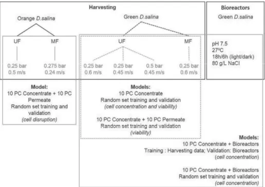
“orange” and “green” cells. For “orange” D. salina, two harvesting experiments were performed, a pilot scale ultrafiltration (UF) and a lab scale microfiltration (MF). For “green” D. salina, four experiments were performed, three UF and one MF. Five lab scale
bioreactors were performed with the same growth conditions. Grey boxes indicate the experiments used to develop the predictive models. ... 17 Figure II.2 2D Fluorescence spectra of the culture at the beginning of the membrane harvesting
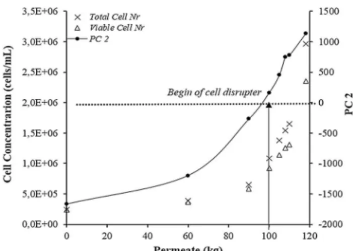
(a), immediately before (b) and after (c) the onset of cell disruption, defined as 10 % decreased of viability when compared to the initial biomass. Three distinct fluorescence regions were identified as I (excitation 275 nm, emission 300-350 nm), II (excitation 350 nm, emission 400 nm) and III (emission higher than 650 nm). ... 18 Figure II.3 Total (x) and viable cell number (Δ) during the membrane harvesting experiment
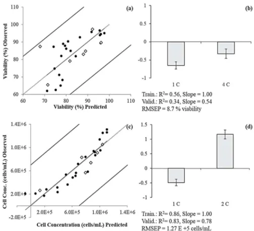
(0.25 bar and 0.6 m/s). PC 2 (●–●) resulted from the PCA applied to the fluorescence EEMs acquired from the concentrate stream. ... 20 Figure II.4 Prediction models and normalized regression coefficients for viability percentage (a
and b, respectively) and cell concentration (c and d, respectively) using PCs from the concentrate only. Training (n=21 for viability and n=22 for cell concentration) (●) and validation (n=7 for viability and n=6 for cell concentration) (◊) data are presented as percentage for viability, and cells/mL for cellular concentration. 1C, 2C and 4C are,
respectively, PC1, PC2 and PC4 from the concentrate spectra. ... 21 Figure II.5 Predicted vs observed values for viability percentage (a), with training (n=21) (●) and
validation (n=7) (◊) values presented, using PCs from the concentrate and the permeate. Regression coefficients (b) are in normalised units. 1C, 2C, 7C, 1P and 2P are,
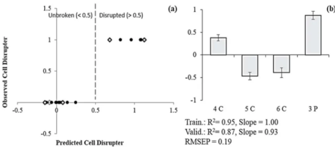
respectively, PC 1, 2, 7 from the concentrate and PC 1 and 2 from the permeate spectra. ... 22 Figure II.6 Prediction model for cell disruption of “orange” culture during harvesting (a), using
PCs from the concentrate and permeate streams. Training (n=13) (●) and validation (n=4) (◊) data are presented as unbroken (< 0.5) and disrupted (> 0.5) cells. Regression coefficients (b) are in normalized units. 4C, 5C, 6C and 3P are, respectively, PC 4, PC 5 and PC6 of the concentrate and PC 3 of the permeate spectra. ... 23 Figure II.7 Cell number prediction model (a) using harvesting experiments as training (n=28) (●)
and bioreactors as validation (n=32) (◊), both in cells/mL. Regression coefficients (b) of model inputs are in normalised units, using PCs from 1 to 10. ... 24 Figure II.8 Cell concentration prediction model (a) using random sets for training (n=45) (●) and
validation (n=15) (◊), both in cells/mL. Regression coefficients (b) of the model inputs are in normalised units, using PC 1 to 10. ... 25
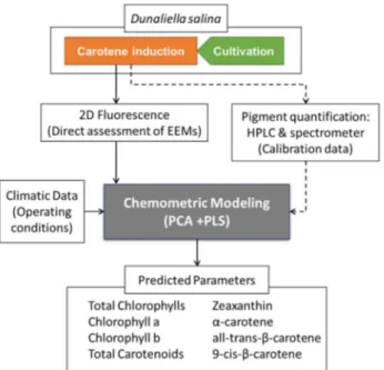
xviii Figure III.1 Schematic representation of the methodology followed. Dashed arrows represent
the off-line measurements required for model calibration. ... 32 Figure III.2 2D Fluorescence spectra of D.salina during the sixth batch; (a) day one
(inoculation), (b) after six days, and (c) after fourteen days. X-axis displays the wavelengths of emission, Y-axis the wavelengths of excitation and the intensity of the fluorescence is represented through color gradient. Two distinct fluorescence regions can be noticed, a protein-like region (excitation wavelength of 275 nm and emission
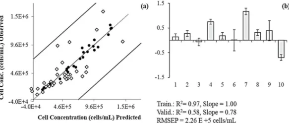
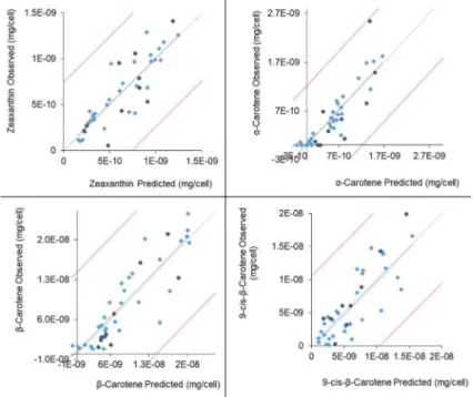
wavelengths between 300 and 350 nm) and a pigment band (emission wavelengths above 650 nm). ... 34 Figure III.3 Carotenoids concentration prediction models, from left to right and top to bottom:
zeaxanthin, α-carotene, β-carotene and 9-cis-β-carotene. Training (◊) and validation (●) data are presented as mg/cell. Statistical parameters of the models represented are displayed in Table III.3. ... 39 Figure IV.1 Schematic representation of the procedure used during the consecutive membrane
harvesting experiments. CF represent the concentration factors during the experiment, calculated in function of mass of biomass, in the beginning of the load (mi) and in the end of the load (mf). ... 47 Figure IV.2 Schematic representation of the overall process and indication of the sampling
points. Samples were withdrawn from cultivation broth and its supernatant, from the concentrate and permeate streams during membrane filtration, and from during permeate treatment. ... 48 Figure IV.3 Fluorescence spectrum of Dunaliella salina biomass, acquired during
carotenogenesis experiments. The emission wavelengths is in the x-axis, the excitation on the y-axis, and the fluorescence intensity in colour-grade scale. Two distinct areas can be identified: protein-like region for excitation wavelengths between 250 and 350 nm, and emission below 300 nm; and the pigment band, for excitation wavelengths above 650 nm through the entire range of emission wavelengths. ... 51 Figure IV.4 Cell concentration prediction models (a) for cultivation experiments samples; (c) for
membrane harvesting experiments, using only PCs acquired in the concentrate stream; and (e) for two distinct processes, cultivation and harvesting, using fluorescence EEMs from both processes compiled together. Respective normalized regression coefficients are shown in (b), (d) and (f), in the same order. Training (◊) and validation (●) data are
presented as cell/mL. Model (a) training set included 31 fluorescence spectra, and 10 for validation set. Model (c) training set included 104 fluorescence spectra, and 34 for validation set. Model (e) training set included 135 fluorescence spectra, and 44 for
validation set. ... 52 Figure IV.5 Prediction models for viability percentage during membrane harvesting experiments:
using ten PCs of the fluorescence acquired in the concentrate stream (a) and adding ten PCs of the fluorescence acquired in the permeate stream to the ten PCs of the
concentrate stream (c). The respective regression coefficients (b and d) are in normalised units. The letters "C" or "P" before the PC number indicates its origin, from concentrate or
xix permeate streams, respectively. Training (◊) (n=104) and validation (●) (n=34) data are presented as percentage of viability. ... 55 Figure V.1 Photobioreactor operating conditions; environmental conditions tested ... 64 Figure V.2 Average biomass concentration and respective standard deviation bars, expressed
as dry weight (g/L), measured over time, from the moment of stress induction. A) For 24h of light and nitrogen starvation, comparison between different temperatures: 15 (circles), 20 (squares), 25 (triangles) and 30 °C (diamonds); B) For day/night cycle (16:8),
comparison between nitrogen starvation (N-starv, triangles), decrease of temperature from 25 to 15 °C (25-15°, circles) and a control experiment (no starvation and no decrease of temperature, squares). ... 67 Figure V.3 EPA content expressed per dry weight of biomass (g EPA/g DW) in the TAG (dark
grey) and PL (light grey) fractions. A) For 24h of light and nitrogen starvation, comparison between different temperatures: 15, 20, 25 and 30 °C. B) For day/night cycle (16:8), comparison between nitrogen starvation (N-starv), decrease in temperature from 25 to 15 °C (25-15) and a control experiment (no starvation and no decrease in temperature); ... 69 Figure V.4 Prediction models of EPA content content (% g/gDW) in TAG fraction of N. oceanica.
In Figure 4, predicted values (x-axis) are plotted against observed values (y-axis). Training (●) and validation (▲) data are represented in percentage of grams of EPA per grams of dry weight. ... 72 Figure V.5 Prediction model of EPA content in TAG fraction using 75 % of the data for training
(●) and 25 % for validation (▲), represented in percentage of grams of EPA per grams of dry weight. Normalised regression coefficient of the represented prediction model. ... 73 Figure V.6 Prediction models of EPA content content (% g/gDW) in PL fraction of N. oceanica. In
Figure 4, predicted values (x-axis) are plotted against observed values (y-axis). Training (●) and validation (▲) data are represented in percentage of grams of EPA per grams of dry weight. ... 74 Figure V.7 Prediction model of EPA content in PL fraction using 75 % of the data for training (●)
and 25 % for validation (▲), represented in percentage of grams of EPA per grams of dry weight. Normalised regression coefficient of the represented prediction model. ... 75 Figure VI.1 Fluorescence spectra of a Nannochloropsis oceanica sample: a) original spectra; b)
final spectra used as inputs in the PLS models. Rayleigh scatter of first order was removed and replaced by empty values; the second order was replaced with an interpolation of surrounding data points. Fluorescence signal corresponding to emission wavelengths (y-axis) shorter than the excitation wavelengths (x-(y-axis) was replaced by zeros. Inner filter effects were also corrected whenever present. ... 82 Figure VI.2 Cell concentration prediction model (one of the four partitions of training/validation
data sets). Training (●) (n=69) and validation (▲) (n=23) data are represented in log10
cells/mL. ... 82 Figure VI.3 Chlorophyll content prediction model (one of the four partitions of training/validation
data sets). Training (●) (n=57) and validation (▲) (n=19) data are represented in log10
xx Figure VI.4 Fatty acids (FA) prediction models for total (a), saturated (b) and unsaturated (c) FA
(one of the four partitions of training/validation data sets). Training (●) (n=54) and
validation (▲) (n=18) data are represented in log10 % g/g DW. ... 85
Figure VI.5 Regression coefficients of the prediction models for cell concentration, chlorophyll, and fatty acids (FA) as total, saturated and unsaturated; 100% of the data set was used as training set. Excitation wavelengths are represented in the x-axis, emission wavelengths in the y-axis, and intensity is represented in the colour bar on the right side... 87
xxi
List of Tables
Table III.1 Climatic parameters used in the development of the PLS models ... 31 Table III.2 Statistical parameters of the selected models for chlorophylls prediction. The climatic
inputs code is shown in Table III.1 ... 35 Table III.3 Statistical parameters of the selected models for carotenoids prediction. The climatic
inputs code is shown in Table III.1 ... 38 Table IV.1 Operational conditions of membrane filtration of D. salina. Parameters tested:
permeate volumetric flux imposed; type of membrane according to the pore size; and membrane relaxation procedure (N - without relaxation, y - 9 minutes of operation and 1 minute of relaxation). A consecutive increment of biomass was performed twice (Y) (n – no biomass increment). ... 46 Table IV.2 Input strategies used for the PLS model construction of cellular concentration,
cellular viability and nitrate concentration prediction, and the corresponding prediction model representation. ... 50 Table IV.3 Statistical parameters of the selected models for nitrate concentration prediction. .. 56 Table V.1 Cell size (µm) of N. oceanica at the first day of the “stress phase”, and after 4 and 10
days. Experimental error inferior than 2.32 % for all measurements. ... 68 Table V.2 Statistical parameters of the prediction models of EPA content (% g/gDW) in TAG
fraction of N. oceanica. ... 72 Table V.3 Statistical parameters of the prediction models of EPA content (% g/gDW) in PL
fraction of N. oceanica. ... 74 Table VI.1 Experimental conditions of the eight batch experiments performed ... 79 Table VI.2 Prediction models parameters for total, saturated and unsaturated fatty acids. ... 86 Table VII.1 Prediction model parameters parameters for EPA in TAG and in PL fractions of N.
oceanica. The results showed are an average of 4 cycles of random validation data sets (25 % of the total data set). The same data sets where used in all prediction models, using raw or pre-treated fluorescence spectra. ... 94
xxiii
List of Acronyms
Abbreviations 2D – Two Dimensional AM – Analytical Method
ANN – Artificial Neural Networks ASW – Artificial Sea Water Car – Carotenoids
Cc – Cell concentration
Chl – Chlorophyll; Chl a – Chlorophyll a, Chl b – Chlorophyll b Cumul. – Cumulative
Cv – Cell viability CV – Cross-Validation DW – Dry Weight
ECMWF – European Centre for Medium-Range Weather EEM – Excitation-Emission Matrix
EPA – Eicosapentaenoic Acid FA – Fatty Acids
Fluor.PCs – Fluorescence PCs
FPAR – Fraction of Photosynthetically Active Radiation IR – Infrared Spectroscopy
ISE – Iterative Stepwise Elimination LOOCV – Leave-One-Out Cross-Validation LV – Latent Variable
MAPLASS – Multivariate Additive PLS Splines MF – Microfiltration
MLR – Multiple Regression Regression
MODIS – Moderate Resolution Imaging Spectroradiometer MTBE – Methyl-tert-butylether
MWCO – Molecular weight cut-off
NIR – Near-to short-wave Infrared Spectroscopy NL – Neutral Lipids
xxiv n-PLS – multiway version of PLS
N-starv – Nitrogen depletion (“starvation”) PAHs – Polycyclic Aromatic Hydrocarbons PAM – Pulse Amplitude Modulated fluorometry PC – Principal Component
PCA – Principal Component Analysis PCR – Principal Component Regression pCO2 – CO2 Partial pressure
PI – Propidium Iodide PL – Polar Lipids
PLS – Projectionto Latent Structures pO2 – O2 Partial pressure
PUFA – Polyunsaturated Fatty Acids R2 – Coefficient of determination
RMSECV – Root Mean Square Error of Cross-Validation RMSEP – Root Mean Square Error of Prediction
ROS – Reactive Oxygen Species Sl – Slope
TAG – Triacylglycerols UF – Ultrafiltration
1
I.
Introduction
I.1. Challenges in monitoring biological systems
Due to the increased interest for greener and renewable bio-based economies, biomass is being valorised for the sustainable production of food and feed, but also chemicals, fuels and power. Through the years, several technological advances have been studied and implemented that increased the competitiveness of biomass production. The introduction of closed cultivation systems, like bioreactors, enabled the production under defined and controlled conditions, leading to optimised viability, reproducibility and higher productivities. Following this trend for more competitive production systems, the need of online monitoring emerged.
Within the biotechnological processes involved in a cell-based biorefinery, three types of parameters need to be monitored: physical, such as temperature and conductivity; chemical, like pH, O2 and CO2 partial pressure (pO2 and pCO2); and biological, as cell concentration and viability
and products concentration. It is important to take into consideration that interactions between those three classes of parameters can occur, and that these interactions are usually complex. Also, in these biological systems, the measured parameters are usually less than the parameters that need to be controlled, increasing the difficulty to monitoring and control the process [1,2]. Currently most of the monitoring is based on off-line analysis of samples withdrawn from the cultivation or biorefinery processes. Usually the sampling frequency is conservative to not disturb the system or contaminate it. All metabolic activities in the sample need to be stopped to reflect the cell status at that specific time. In addition, some results depend on time consuming analytical procedures, making this sampling strategy not appropriate for direct process control [3].
Therefore, online monitoring and a closer process control of bioreactors is a basic requirement for the development of efficient biological processes [4,5]. With online sensors it is possible to acquire a continuous stream of information with short response times. In this way, biological systems can be monitored faster and more efficiently, allowing an immediate response, if needed. This increases the control on production, leading to an improved production processes with a high-quality control.
The selection of the right sensor for the online monitoring of biological processes must match the needs of the bioprocess in question. The most general requirements are selectivity, sensitivity and response time [2,6,7]. Accordingly to Glindkamp et al. [2] three configurations have been explored so far: in situ, where the medium is monitored directly; online, when the sensor is moved to a particular part of the bioreactor, like a bypass, so the bubbles from aeration do not interfere (for example); and off-line, removed from the bioreactor.
Nowadays, the most common in situ and online sensors used in biotechnology are based in electrochemical principles like pH, pO2, conductivity, and are well-known in the field. However, the need of an efficient tool to monitor simultaneously a wider range of substrates and products,
2 and to control the cultivation environment, increased the urgency for better solutions, and the use of optical sensors for in situ and online monitoring is emerging.
I.2. Optical sensors - Techniques available
With the development of better optical fibres, able to be used in larger distances and in longer communication ranges, the optical sensor technology became very promising for online monitoring. The principle of spectroscopic optical fibre sensors is based on the interaction between light waves (absorption or luminescence) with the molecules. This technique presents several advantages for online monitoring of complex biological systems, as for example industrial microalgae production and refinery. These sensors are non-invasive, non-destructive and allow the detection of several different molecules simultaneously. The need for sampling the system is low or inexistent, so it decreases the culture contamination, and no time delay is observed when acquiring the data, making them a great solution for real-time monitoring. Also, as non-invasive techniques, they will not interfere with the biological material, allowing to monitor in vivo cells and obtain information about their intracellular state, in addition to information about extracellular media [1,2,4,8].
The spectroscopic optical fibre sensors can be divided in four categories based on the way they interact with the sample. They can be used combined with an indicator for specific molecules (usually fluorescent dyes) [1], coupled to a biological receptor like a catalytic effect (enzyme-based) or comprise immune and gene sensors (antibodies) [4], or, in the most simple case, analyse the optical properties of the sample [9]. This last approach is more adequate when aiming to monitor microalgae cultivation and biorefinery online, since no interaction with the culture is required and several metabolites can be analysed at the same time.
Most spectroscopic methods, including infrared, Raman and fluorescence spectroscopies, have been study for (bio)processes monitoring, often in combination with optical fibres [9].
I.2.1. Infrared spectroscopy
Infrared (IR) spectroscopy has been used in bioprocess monitoring for the measurement of several metabolites, such as ethanol, glucose and fructose. Since most bioprocesses take place in aqueous medium, and due to the huge IR absorbance of water (for wavelengths higher than 2500 nm), this technique can only be applied with a short optical path length or in the range of near-to short-wave IR range (NIR), from 780 to 2500 nm [2].
NIR spectroscopy provides information about the structure composition of the molecules (position, shape and size) through the detection of the biological bonds C-H, N-H, O-H and S-H. The absorption bands can be weak and similar, can also be broad or overlap. Each molecule in the sample can absorb at more than one wavelength, and each wavelength can have multiple contributions from the different molecules present in a sample. For this reason, a direct spectra interpretation is not possible, being necessary the use of advanced data analysis to extract the information embedded in spectra. However, the restrictions of this technique also bring advantages. The low absorption coefficients enable a higher penetration depth, allowing the use
3 of this technique in solids or turbid liquids, such as culture broths [1–4]. NIR spectroscopy, coupled with an optical probe, was used to monitor cell density online through light absorption (turbidity) or scattering, in the visible and/or NIR range. However, the inability to distinguish viable from non-viable cells, the narrow cell concentration range where can be applied, and the sensitivity towards different morphologies, are some of the restrains that need to be improved for the use of this spectroscopy as an online monitoring tool [4].
I.2.2. Raman spectroscopy
Unlike IR spectroscopy, that is being used in industrial proposes for several years, Raman spectroscopy is still in the stage of academic research [10].
Raman spectroscopy is based on the phenomena of shifted wavelength scattering of molecules excited with monochromatic light due to inelastic collisions of photons with the molecule [1]. This technology does not require clear samples, increasing the spectrum of usage in biotechnology industries. Additionally, with the development of Fourier-transform, the acquisition times and the photodecomposition were considerably decreased. Nevertheless, the intensity of the signal acquired is very weak and difficult to separate from the scattering [10].
Nowadays, several Raman methodologies are being studied to replace the standard procedures, such as GC or HPLC, for quality control and confirm adulterations of several products, like microorganisms, food products or even pesticides [10].
I.2.3. Fluorescence spectroscopy: principles
Luminescence, the phenomenon of light emission, can be divided into two categories, phosphorescence and fluorescence. Fluorescence occurs when an excited singlet state, in which an electron is paired by opposite spin to another electron from the ground-state orbital, returns to its ground state by the rapidly emission of a photon [11,12].
The first fluorescence sensors developed enabled only one wavelength of excitation and emission, meaning that only one fluorophore could be measured, restricting the use of this technology in complex processes. Later on, the development of multi wavelength fluorescence sensors make it possible to detect simultaneously several fluorophores in the same measurement, boosting the use of fluorescence spectroscopy as a scanning technique [1,2,11,13]. The measurement of several emission wavelengths over a range of excitation wavelengths creates a 2 dimensional (2D) excitation-emission matrix (EEM), that can be plotted in 3D graphs through the intensity recorded for each excitation-emission pair [4,12,14–16].
Fluorescence spectroscopy is a non-invasive technique, with high sensitive detection and specificity, able to detect instantaneously several natural fluorophores. These fluorophores can be classified into two main categories, extrinsic and intrinsic. Extrinsic fluorophores are the ones that need to be added to a sample that naturally does not possess fluorescence, such as fluorescein and rhodamine, among others. Intrinsic fluorophores are compounds that occur naturally in nature, such as NAD(p)H, chlorophyll, amino acids, cofactors and vitamins [4,8,11,12,14,17].
4 This technique is sensitive to intracellular and extracellular metabolites and media composition. In biological systems, characterised for having rich media composition, the interaction fluorophore-media is rather complex, since parameters like the polarity of the media, fluorophores structure and the interaction between them and with nearby molecules can cause a shift in the spectra. The phenomenon of masking the response of the fluorescence intensity of natural fluorophores is called quenching. Quenching can be collisional or static, if the decrease in the fluorescence is achieved by contact with another fluorophore or when forming a non-fluorescent complex, respectively [1,12]. For this reason, it was reported the use of fluorescence to indirectly determinate non-fluorescent compounds, since their presence can interfere with the fluorescence captured, and therefore, create a finger-print in the fluorescence spectra [1]. A different phenomenon is the inner-filter effect, also mentioned as self-absorption, where the fluorescence light is absorbed by the fluorophore itself [18]. It is also noteworthy that very dilute solutions will present a higher scatter interference in the EEMs due to the interaction between water molecules and the fluorophores. Two types of scatter can be notice: 1st and 2nd order
Rayleigh, when the emission equals the excitation or two times the excitation, respectively, and Raman, with shift to longer wavelengths called red shift [19,20].
I.2.4. Fluorescence spectroscopy: biochemical applications
The urge for a rapid and online technology in the bioprocess industry, but also in environmental or clinic applications, accelerated the research and development of a system that could be coupled to a bioreactor, via optical fibre, and that could give an answer at real time.
Several authors have been studying the use of fluorescence spectroscopy to monitor online conventional fermentations. Most of the reported cases investigate the fluorescence of the reduced form of NAD(P)H, which fingerprint is detected at an excitation wavelength of 340 nm and emission wavelength of 460 nm. NADH is a highly fluorescent molecule, and it is known that the fluorescence intensity signal has a good correlation with the biomass concentration and its metabolic state [4,5,14,21]. For that reason, fluorescence spectroscopy was been used to track physiological changes, such as the transition between bacterial aerobic and anaerobic metabolisms [2], and also the change between oxidative and oxidoreductive metabolism in yeasts [8]. Fluorescence spectroscopy was also used to monitor biomass and substrates or products concentrations in E. coli and S. cerevisiae fermentations [4,17].
It is well reported in the literature the versatility of fluorescence spectroscopy to monitor several analytes, through direct or indirect correlations, such as proteins, vitamins, co-enzymes, and several metabolites such as glucose, ethanol, ATP, pyruvate, nitrate or succinate [1,2,8,11,22]. A system developed by the company DELTA Light & Optics (Lyngby, Denmark), called BioView™, was used to predict several cultivation parameters, such as enzyme activity, product formation and substrate consumption, with the final goal of defining an optimal harvest time [13,21].
Fluorescence spectroscopy has also been studied as a monitoring tool in several fields of the food industry such as the industrial downstream processing of sugar beet molasses [1], the characterization and classification of honeys [15], or the detection of orange juice frauds [23]. Other applications under study include in situ characterization of polycyclic aromatic hydrocarbons (PAHs) [24], or even as a sensor to detect illegal drugs (cocaine and marijuana) in street samples [25], which shows the versatility of this technique. In the pharmaceutical field, fluorescence
5 spectroscopy was studied as a monitoring tool for the physiological state of mammalian cell cultures, a platform for the production of anti-bodies, blood and growth factors or cytokines [26]. Also, several studies reported the potential of using this technique in wastewater treatment plants [27–32]. Ranzan et al. [11] stated that the application of this technology as a monitoring tool in biological systems proved to improve the ecological and economic management of the overall process under study. More applications can be found in the review of Pons et al. [21].
In the scientific fields of terrestrial plants and microalgae, the use of fluorescence was studied through Pulse Amplitude Modulated (PAM) fluorometry. This technique enables the measurement of chlorophyll a fluorescence and photosynthetic performance, both in growth and stress phases [33].
Although a major advance was observed in the quality of the optical sensors used in spectroscopy methodologies, these sensors are still rarely used in biotechnology industry, and most of the devices developed have been only study for research purposes [1,4]. The main concerns reported for the limited application of this technology are mostly due to interferences that affect the quality of the fluorescence spectra acquired, such as turbidity, gas bubbles and fouling [1,4,14].
I.3. Chemometrics: mathematical treatment of the spectra information
The first records of chemometrics were reported by Mandel in 1949, but only nearly 25 years later the term “chemometrics” itself was invented [34]. According to the Chemometrics Society, chemometrics is “the chemical discipline that uses mathematical and statistical methods to design or select optimal procedures and experiments, and to provide maximum chemical information by analysing chemical data”.
A full fluorescence spectra can contain in-depth information about a biological system under monitoring and it is usually complex, since it contains information about the natural fluorophores present in the sample, but also the interferences between them and the environmental media [4,5]. For that reason, chemometric methods are often used to deconvolute the information within the fluorescence matrices, and to determine the relationship between them and the concentration of substrates and products to be monitored [3,26,29].
Multivariate analysis, like Principal Component Analysis (PCA), is often used to extract the meaningful information from the spectra. PCA reduces the dimension of the data set by extracting the most relevant information. For a n number of initial variables (X1, X2, …, Xn), n linear
combinations are obtained, the so-called Principal Components (PCs), characterized for being uncorrelated and ordered according to the variance explained (the first PC explains the higher part of the variance, and smaller parts of variance are explained with subsequent components) [16,35]. The principle that no correlations exist between PCs is of most importance, since in that way it is guaranteed that each PC describes different patterns of the original data. After the identification of the first PC, the second one is calculated according to the direction that explains more residual variance and with a constrain of being orthogonal to the first one. The process continues until n PCs are defined. In the end, the PCA defines the initial data set (the matrix X) as X=T.PT + E, where T matrix is the scores matrix (represents the objects in the new orthogonal
6 space), P matrix is the loadings matrix (represents the importance of each variable), and E is the error (residuals) matrix (contains the difference between the observed values and the ones predicted by the PCA). An important step to define the new set of variables through the PCA is the normalization, achieved by the subtraction of the mean value to the variable followed by the division by the standard deviation [16,35,36]. This procedure enables the comparison of variables that originally present different magnitudes and variances in a new reduced orthogonal space.
Most of the chemometric applications in analytical chemistry and biochemistry are prediction models, since the use spectral measurements to replace time-consuming chemical and biological lab analysis is very appealing. In other words, chemometric models are often used to find the correlations between a bio-/chemical variable (called dependent variable, y) and the data acquired from instruments such as a spectrofluorometer (independent variable, x) [37]. This relationship established between the dependent variable and a set of independent variables will be used as a linear polynomial prediction model, defined as 𝑦 = 𝑏 + 𝑏 𝑥 + 𝑏 𝑥 + ⋯ + 𝑏 𝑥 + 𝑓, where b0 is an offset, bk (k=1, …, K) are regression coefficients and f is the residual. To calculate
b, the vector of the regression coefficients, multiple linear regression (MLR) is often used. However, the use of MLR requires uncorrelated spectral variables (x-variables), and in fluorescence spectra it is frequent to find collinearity in the x-variables and, also, matrices are often constituted by more variables than objects. A solution often used is to apply MLR analysis to PCA scores, technique denominated principal component regression (PCR), where PC’s that explain high variability in the spectra are correlated with the target properties (y). Another multivariate regression model used frequently for fluorescence data analysis is the projection to latent structures (PLS). This differs from the PCR analysis since it find the correlations that best describe the highest variation between spectral (x-variables) and target properties (y) with a new set of axes (latent variables – LV) [2,4,11,14,16,35,38].
When is not possible to establish a linear relation between inputs and outputs, the regression methods fail to develop prediction models. Thus, the use of nonlinear methodologies may be helpful to model more complex relationships, such as multivariate additive PLS splines (MAPLASS) or artificial neural networks (ANN) [39]. Briefly, ANN embodies a “machine-learning” algorithm that attempts to mimic the information processing found in the human brain, using artifical “learning-from-experience”. Detailed information about ANN can be found elsewhere [32,39–41].
When evaluating the quality and suitability of a prediction model, several parameters need to be assessed:
1) Variables selection: Not all the variables of the data set contribute with useful information for the model. The use of too many variables leads to overfitting, which means a false increase of the variance explained; the use of few variables leads to under fitting, which can result in the loss of relevant information. For that reason, several mathematical methods can be used to find the number of variables that better describe a model, such as iterative stepwise elimination (ISE) [42], stepwise elimination [43] and the Martens uncertainty test [43] using jack knife standard deviations [44].
2) Calibration (Training): From all the data set acquired, a part of the data is select to build the model, called the calibration or training data set. This data set should be representative of the range of all data acquired, and for this, random choice is often the best strategy. A
7 model can be evaluated through the percentage of variance explained, which means, how much variability it captures; and through the root mean square error of calibration (RMSEC), providing information about the magnitude of the error. To test the quality of the model developed, a cross-validation (CV) strategy can be used. Basically, several models are developed using another independent set of data, or leave one or n data points out (LOO and LNO, respectively), and repeatedly evaluate the error of the models (RMSECV). The importance of the calibration relies on the future usage of the model, when a new set of values will be computed through the model developed [35].
3) Validation (Test): To determine if a model is reliable, validation it’s a crucial step of the process. It is expected that the model fit the initial assumptions and that defines the parameters under study, that is stable when a new data set is used for the prediction, and that the correct number of PCs were chosen. To validate the model developed with the calibration data set previously described, a new data set is selected, that was not used to build the model itself (validation set or test set), and the correspondent residuals are calculated. The distance, on average, from the data point observed and the prediction obtained with the model can be evaluated through the root-mean-square error of prediction (RMSEP) [37].
With the development of new technologies and instrumentation able to produce a continuous flow of information, an expansion is being observed in several omics’ fields. The possibility of having a clear insight in biochemical processes and reactions revealed to be a powerful tool for the industries. Workman Jr. [45] presented several advantages of using chemometrics, among them:
1) Allows the possibility of providing real-time and high-quality information from less data 2) Improves the existing knowledge of the processes under study and enables the
improvement of measurements 3) Requires low capital investment
The combination of spectrophotometric instruments with their high sensitivity and resolution, like fluorescence spectroscopy, coupled with chemometrics analysis for comprehension, data pre-treatment and exploration, enhances the knowledge and control of the processes.
I.4. Case study: microalgae production and added-value products
formation
Microalgae are well-known photosynthetic microorganisms with the ability to produce a wide variety of value-added metabolites with the use of sunlight and CO2 fixation, from the atmosphere
or fume gas. When comparing microalgae to other plant crops they present several advantages: they have higher photosynthetic conversion efficiencies and higher biomass production rates, they can grow in diverse and inhospitable environments, they don’t compete for land and can be grown in sea water [46]. However, nowadays, microalgae production is far from the terrestrial crops, since the production capacity of microalgae is still done in niche markets for high value
8 products. Their industrial production costs need to be reduced and the scale needs to increase to make this industry more competitive [47,48]. Mostly of the industrial facilities are based in open ponds systems, being only a few produced in closed photobioreactors. Being the growth and productivity of microalgae cultivation so tightly correlated with light conditions, better engineering solutions have to be developed regarding light distribution, mass transfer and hydrodynamics [48,49]. Operational costs are still too high and dependable on the local conditions and the metabolites produced for commercialization [48].
By minimizing the production and processing costs of microalgae biomass, the production costs of microalgae products will decrease. New technologies developed need to be easily scalable, but they also need to be competitive in operational and investment costs. To increase the economical yield of this industry, a biorefinery approach has been proposed where, instead of focusing in a specific product, a portfolio of products can be extracted, separated and purified according to its end market [47].
In a microalgae biorefinery production, the entire value chain is connected. Higher product yields require both high biomass productivity and high efficiencies in harvesting and biomass processing. Microalgae cultivation is mostly done in very diluted biomass concentrations, from 0.2 to 2 g/l, to avoid a large dark zone in the cultivation system, which leads to low productivities [50,51]. This low biomass concentration with consequent large volumes, leads to high dewatering costs. The most common technology used for dewatering microalgae biomass is centrifugation, which is a very energetic demanding technology [52]. To reduce harvesting costs, two-step harvesting processes are being studied, as for example, using membrane filtration as a primary dewatering step before centrifugation [52,53]. The possibility of using this technology enables also the recovery and recirculation of the cultivation media, which represents a positive economic impact on the overall costs of microalgae biomass production. However, this harvesting step is particularly sensitive for several algae that lack rigid cell wall. Within a biorefinery concept, the importance of maintaining the cell integrity is directly proportional to the product yield that can be recovered from its biomass.
Microalgae cultivation is a complex production system in which several biological, fluid dynamics, environmental and nutritional conditions play a crucial role in the productivity and viability of the industrial process. For these reasons, the development of prediction models that allow online monitoring of substrates and products is fundamental for process control, enabling the possibility to take decisions and actions at real-time [49]. In the present work, two marine microalgae were studied, Dunaliella salina and Nannochloropsis oceanica. Both microalgae genus are currently produced industrially and are authorized for food and feed supplements. Thus, having an online monitoring tool would be of great interest, not only to monitor the cultivation process, but also the induction of their respective target compounds and their biomass harvest.
The industrial production of Dunaliella salina is one success case in the microalgae biorefinery. This halotolerant microalgae has the ability to produce high contents of carotenoids, around 10% of the total dry weight, under stress conditions as high salinity, high light intensity, nutrient depletion or extreme temperatures [54–56]. Carotenoids are light-harvesting pigments and reactive oxygen species (ROS) scavengers, they act as non-photochemical quenching, which means they absorb the excess light preventing damage on the photosynthetic apparatus. In the actual market, the global market of carotenoids reached nearly $1.5 billion in 2017 and should
9 reach $2.0 billion by 2022 [57]. The cultivation systems more often used for D. salina cultivation are large unstirred open ponds or paddlewheel stirred raceways. A two-step cultivation is commonly applied: the first stage, a “green” phase, where growth is done under optimal conditions; a second stage, the “orange” phase, where the culture is submitted to stress factors and the carotenoid production is enhanced [58]. Regarding D. salina harvesting, studies have been made to present more efficient processes, either economically or sustainably, since this microalga is highly sensitive to shear stress due to the lack of rigid cell wall, compromising the overall profit of the process [51,53].
Several Nannochloropsis species gained interest because of their known ability to produce and accumulate large amounts of lipids, between 25 and 45% of their total dry weight. This made Nannochloropsis sp. production of great potential for biofuel production but also for food supplements, due to the high concentration of omega-3 fatty acids like eicosapentaenoic acid (EPA) [59]. When this microalga is submitted to environmental stresses, like high light intensity and/or nitrogen depletion, it has the ability of storing triacylglycerol (TAG) compounds in lipid bodies. Several companies already produce Nannochloropsis sp. in outdoors facilities, usually following a two-step strategy: an initial growth phase under optimal conditions is followed by nitrogen depletion to induce the accumulation of fatty acids [60]. It is hypothesized that TAG accumulation helps the prevention of photo-oxidative stress, helps regenerate NADPH to NADP+, and storages chloroplast components to be used when favourable growing conditions are restored [61].
I.5. Thesis motivation and outline
I.5.1. Motivation
The main objective of this thesis is the development of an online monitoring tool able to be used in microalgae production, that enable the monitoring of several parameters simultaneously and different processes within the production. Two marine microalgae are studied, known for their capacity to produce compounds of interest for food and feed, under growth and stress conditions: D. salina for its capacity to accumulate carotenoids, and N. oceanica for its capacity to accumulate fatty acids. Five parameters are monitored – cell concentration, cell viability, pigments concentration, fatty acids composition and nitrogen concentration – in four different processes – cultivation, product formation (carotenoids and lipids), harvesting by membrane filtration and permeate recover. A schematic illustration of the questions and studies developed in this work are shown in Figure I.1.
To prove the potential of fluorescence spectroscopy coupled with chemometric modelling techniques, different approaches are studied. The EEM of the spectra are used raw, without pre-treatment for removal of the scatter and inner-filter effects, and with pre-treated EEM. Two input strategies are performed in the PLS modelling, using the PC’s resulting from a PCA performed on the EEM, or directly using the EEM. More detailed information about the different approaches are explained throughout the thesis.
10 Figure I.1 Schematic illustration of the questions and studies performed in this thesis. Cc – Cell concentration; Cv – Cell viability; Chl – Chlorophyll; Car – Carotenoids; N – Nitrogen; FA – Fatty Acids.
I.5.2. Thesis outline
This PhD thesis comprise the following chapters:
Chapter 1 – Introduction: a state of the art is provided to present the current challenges of monitoring biological systems, such as microalgae, and the use of optical sensors coupled with chemometric tools as a solution.
Chapter 2 – 2D Fluorescence spectroscopy for monitoring Dunaliella salina concentration and integrity during membrane harvesting: D. salina is well-known for the production of carotenoids, when in its “stress-phase”. However, “non-stressed” cells are also rich in salt-tolerant proteins and reactive oxygen species (ROS) enzymes. Due to the lack of rigid cell wall, this microalga can easily disrupt during harvesting, losing valuable compounds to the saline water, affecting the downstream processing. Thus, monitoring cell concentration and integrity in real-time, of “green” D. salina cells, can assist the development and optimisation of harvesting methodologies.
Chapter 3 – Development of a monitoring tool based on fluorescence and climatic data for pigments profile estimation in Dunaliella salina: D. salina pigments profile were monitored, from a “green” (chlorophylls) to “orange” (carotenoids), in order to develop a tool able to be used online in the carotenogenesis step of D. salina production. Climatic parameters were also used as input variables due to their impact on the pigments profile in outdoor cultivations.
Chapter 4 – One tool for simultaneous monitoring of cell concentration, cell viability and nitrogen during production and harvesting of stress-induced Dunaliella salina: Fluorescence spectroscopy was studied as a potential monitoring tool in a biorefinery of D. salina for carotenoids
11 production. Three different parameters were monitored – cell concentration, cell viability and nitrogen concentration - in three different process – cultivation, membrane harvesting and permeate treatment.
Chapter 5 – Monitoring of eicosapentaenoic acid (EPA) production in the microalgae Nannochloropsis oceanica: An alternative source of omega-3 fatty acids is of great importance for the food and feedd industries. Eicosapentaenoic acid (EPA) accumulation by N. oceanica was evaluated through different environmental cultivation conditions – temperature, light cycle and nitrogen repletion/depletion – and a tool based on fluorescence spectroscopy was developed to monitor this fatty acid in the apolar (TAG) and polar (PL) fractions of the cell during cultivation and induction.
Chapter 6 – Fluorescence spectroscopy coupled with chemometric modelling for the simultaneously monitoring of cell concentration, chlorophyll and fatty acids: In a N. oceanica biorefinery, fatty acids are the main product of interest, that can be used for food, feed or biodiesel. During cultivation, the possibility to monitor several parameters simultaneously will contribute to better harvesting-time decision-making. Thus, prediction models for cell concentration, chlorophyll and fatty acids – as total, saturated and unsaturated – were developed.
Chapter 7 – Thesis overview and general conclusions: an overall conclusion of the results achieved throughout this work is presented, as well as suggestions for future work.
13
II.
2D Fluorescence spectroscopy for
monitoring Dunaliella salina
concentration and integrity during
membrane harvesting
Abstract
Dunaliella salina is able to produce simultaneously several valuable compounds (such as lipids, carotenes and functional proteins) within the biorefinery concept. However due to the lack of rigid cell wall, this microalga can easily disrupt during harvesting, losing valuable compounds to the saline water, affecting the downstream processing. Therefore, the development of non-invasive tools able to monitor cell concentration and integrity at real-time, can assist the development of harvesting methodologies. In the present work, a monitoring approach was developed based on two-dimensional (2D) fluorescence spectroscopy. Mathematical analysis of the monitoring data involved the use of Principal Component Analysis (PCA) and Projection to Latent Structures (PLS) modelling. For green D. salina, the models developed for prediction of cell number and percentage of viability captured 90.6 % and 86.3 % of variance, respectively. Both models have R2 of 0.8 and 0.9, respectively for validation and training. Similar values were
found for the prediction of cell number when using data from growth kinetics and harvesting combined. Orange D. salina rupture was also successfully modelled with 95 % of variance captured and R2 of 0.9 for both training and validation. The combined approach using 2D
fluorescence spectroscopy and the mathematical analysis proved to have the potential to monitor D. salina during cell growth and harvesting within a biorefinery concept.
Keywords: Dunaliella salina, 2D fluorescence spectroscopy, Ultrafiltration, Microfiltration, PLS modelling, Monitoring
II
Published as: Sá, M., Monte, J., Brazinha, C., Galinha, C. F., Crespo, J. G., 2017. 2D Fluorescence spectroscopy for monitoring Dunaliella salina concentration and integrity during membrane harvesting. Algal Research, 24:325–332.