CROSSING MOUNTAINS:
THE EFFECT OF COMPETITION ON THE LAFFER CURVE
por
Hugo Miguel de Oliveira Cruz Pinto de Abreu
Dissertação de Mestrado
em Finanças e Fiscalidade
Orientada por
Professor Doutor Samuel Cruz Alves Pereira
Professor Doutor Elísio Fernando Moreira Brandão
i
NOTA BIOGRÁFICA
Hugo Pinto de Abreu nasceu no Porto, a 30 de setembro de 1988. Durante todo o Ensino Básico e Secundário frequentou a Escola Salesiana do Porto, onde foi Presidente da Associação de Estudantes, no ano letivo de 2005-2006.
Em 2006 recebe o 5.º prémio na segunda edição do Prémio Universidade Católica Portuguesa / Xavier Pintado para melhor ensaio económico.
Licenciou-se em Economia em 2009 pela Nova School of Business and Economics. Tendo obtido experiência profissional no setor financeiro e empresarial, em 2011 inicia o segundo ciclo de estudos superiores, ingressando no Mestrado em Finanças e Fiscalidade da Faculdade de Economia do Porto.
Em 2012, ganha o prémio “Young Tax Professional of the Year” da consultora Ernst & Young, representando Portugal na final internacional desta competição, em Boston, onde lhe é atribuído o “Inclusive Leadership Award”. No mesmo ano, vence o prémio de melhor ensaio na categoria de Contabilidade no VIII Ciclo de Temas de Economia, organizado pela Direção Regional Norte da Ordem dos Economistas.
É membro do Conselho Pedagógico da Faculdade de Economia do Porto, e participou, em 2013, nos processos com vista à acreditação EQUIS e A3ES desta Faculdade.
A nível extracurricular, Hugo Pinto de Abreu é voluntário no Centro Comunitário de São Cirilo, no Porto, e Tesoureiro da Associação Una Voce Portugal, de âmbito cultural.
ii
NOTA DE AGRADECIMENTO
“Because our expression is imperfect we need friendship to fill up the imperfections.” – G. K. Chesterton Encontro-me profundamente reconhecido ao Diretor do Mestrado em Finanças e Fiscalidade e Coorientador da presente dissertação, o Professor Doutor Elísio Brandão, bem como ao Orientador, o Professor Doutor Samuel Pereira, pelo aconselhamento e acompanhamento permanentes, pelo seu espírito de exigência e de melhoria contínua, um espírito que procurei interiorizar e ao qual me proponho sempre corresponder.
Estou outrossim reconhecido ao Professor Doutor Vitorino Martins e ao Professor Doutor António Cerqueira, pelas sempre pertinentes observações, análises e sugestões que contribuíram de forma significativa para melhorar este trabalho.
Gostaria, ao centrar-me em agradecimentos de cariz mais pessoal, de referir em primeiro lugar o Dr. Artur Veloso Vieira, que pela sua amizade, incentivo e acompanhamento foi indispensável para a concretização de todo este projeto.
Agradeço aos meus pais, irmã e avós, pelo inestimável apoio em tantas e tão diversas formas e ocasiões.
Ao longo destes anos, foram muitos os amigos que me apoiaram grandemente, ora com os seus conselhos e ajuda, ora com a sua presença simples e afetuosa. Sem pretender de modo algum fazer uma lista exaustiva, gostaria de agradecer muito particularmente à Dra. Beatriz Lobo d’Ávila, à Dra. Ana Sofia Carrapa, ao Eng.º T.º Marco da Vinha e sua esposa, ao Mestre João Bettencourt da Câmara, à Dra. Fátima de Castro, ao Mestre Diogo de Carvalho, à Mestre Andreia Morris Mendes, ao Mário Rocha, ao Mestre Nuno Pinheiro e à Dra. Mariana da Costa Macedo.
iii
RESUMO
Considerando os Estados e outras entidades políticas como produtores e os impostos como um preço, este estudo faz a ligação entre os efeitos, sobejamente estudados na Microeconomia, das estruturas de mercado e a controversa Curva de Laffer, sugerindo que o resultado do “mercado de impostos” depende também da competição. Estudando os determinantes da receita do Imposto Municipal sobre Imóveis (IMI) para os 308 municípios Portugueses, é desenvolvido um modelo geral que explica com sucesso a receita fiscal. É encontrada alguma evidência estatística para a existência, na amostra, de uma Curva de Laffer com múltiplos máximos, e vários testes indicam que a competição influencia – deslocando mas também alterando – a Curva de Laffer, fazendo com que municípios mais competitivos maximizem a sua receita fiscal com taxas de imposto mais reduzidas – i.e. com um preço mais reduzido – que aqueles em ambientes mais monopolistas.
ABSTRACT
Regarding states and state-like entities as producers and taxation as a price, this study connects the thoroughly studied impacts of the market structures in microeconomics to the controversial Laffer curve, suggesting that the outcome of the “taxation market” depends also on competition. By studying the determinants for Property Tax revenue for the 308 Portuguese municipalities, a general model that successfully explains tax revenue is developed. Some evidence is found for the existence of a multiple-peaked Laffer curve in the sample, and various tests indicate that competition impacts – shifting but also changing – the Laffer curve, causing more competitive municipalities to maximize revenue at lower tax rates – i.e. lower prices – than those in a more monopolistic setting.
KEYWORDS
Laffer curve, Taxation, Market Structure, Competition, Municipalities, Portugal
JELCLASSIFICATION
iv
CONTENTS
1. INTRODUCTION ... 1
2. RELATED LITERATURE ... 7
3. PROPERTY TAX AND PORTUGUESE MUNICIPALITIES ... 9
4. DATA AND DESCRIPTIVE STATISTICS ... 11
4.1 Data ... 11
4.2 Control Variables ... 11
4.3 Tax Rates ... 13
4.4 Competition Levels... 14
4.5 Summary Statistics ... 16
5. THE LAFFER CURVE AND THE DETERMINANTS OF PROPERTY TAX REVENUE ... 18
5.1 Testing the Laffer Hypothesis ... 18
5.2 The Laffer Curve Shape Controversies ... 19
5.3 The Laffer Curve through Rate-Revenue Models ... 20
5.4 Estimation Results ... 21
6. THE COMPETITION EFFECT AND THE LAFFER CURVE ... 28
6.1 The Quest for the Competition Effect ... 28
6.2 An Earthquake, Two Mountains? ... 29
6.3 Estimation Results ... 30
7. CONCLUSIONS ... 39
8. APPENDIX A:DESCRIPTIVE STATISTICS SEGMENTED BY COMPETITIVE LEVEL ... 41
9. APPENDIX B:SIMPLIFIED GENERAL MODEL ... 42
10. APPENDIX C:USE OF THE GENERAL MODELS TO PREDICT PROPERTY TAX REVENUE ... 44
v TABLE INDEX TABLE 1……….12 TABLE 2……….13 TABLE 3……….15 TABLE 4……….17 TABLE 5……….22 TABLE 6……….31 TABLE 7……….35 TABLE 8……….41 TABLE 9……….43 GRAPHIC INDEX GRAPHIC 1……….25 GRAPHIC 2……….25 GRAPHIC 3……….26 GRAPHIC 4……….32 GRAPHIC 5……….33 GRAPHIC 6……….36 GRAPHIC 7……….37 GRAPHIC 8……….37 GRAPHIC 9……….38
1
1. INTRODUCTION
Why did Arthur Laffer’s schematic drawing of a curve – a mountain-resembling curve that would forever bear his name - on a napkin of a New York’s restaurant in 1974, have such an impact as to influence notable political platforms and economic teaching alike, becoming a benchmark of supply-side economics? This question deserves careful analysis, especially if we consider that the essence of the Laffer effect, i.e. that beyond a certain point, an increase in the tax rate may cause a fall of tax revenue, had been known for centuries, a notable example being the Confederate “tariff clause”1
. The reason may be that, in its pragmatic simplicity, the Laffer curve contains a powerful lesson, which although it might not always apply in each objective situation, nevertheless gives us notable insights about human behavior and its response to taxation.
Much research has been done in order to gain a better understanding of the Laffer curve and, among many “minor” explanations, two major effects are pointed, namely: the elasticity of the supply of labor and capital, i.e., as taxes rise, there may be less incentives to work or invest; tax evasion, as higher taxes provide incentives for economic agents to move to the informal economy, and, if they reach a certain level, the fairness of the tax, and thus the ethic duty to pay it, may come into question, to a point where tax evasion may be socially accepted and even applauded2. However, most analyses on the Laffer curve tend to focus on how the Laffer curve comes into being, and not on what the Laffer curve is, and, perhaps due to this, have forgotten, or at least insufficiently explored, what may prove to be a major explanation for the Laffer curve, which is the market structure of taxation, or, as we will call it, the “competition effect”.
The main goal of this study is precisely to gain insights about whether and how the market structure of the taxation market impacts the outcome of taxation in general and the Laffer curve, which is a specific representation of taxation outcomes – in particular. Does greater (lesser) competition lead to lower (higher) prices? Can the Laffer curve represent the outcomes of the taxation market? If it can, what shape does that Laffer curve have – classical,
1 This “tariff clause” (Article I, Section 8, Clause 1 of the Constitution of the Confederate States of America,
adopted on March 11, 1861) is analyzed by McGuire and Cott (2002), who show its significance as a predecessor to Laffer’s insight, especially in contrast with the analogous clause of the United States Constitution.
2
2
asymmetrically one-peaked, two-peaked, multiple-peaked? –, and how does competition affect its shape?
Indeed, taxation can be seen as one – usually, the major – price for the existence and the maintenance of a state or of a state-like entity, and for the services it provides to its citizens, which may be more or less extensive. Thus, to a certain extent – and to a certain extent only – taxation can be analyzed as a market where consumers, i.e. taxpayers, demand certain goods (e.g. safety, rule of law), from certain producers, i.e. state or state-like entities3. The Laffer curve is simply the representation, from the producer’s perspective, of the possible outcomes (i.e. levels of revenue), according to different prices (i.e. tax levels) that result from the aforementioned market-like interaction.
The competitive structure of a market will influence its possible outcomes, i.e. price, quantity, consumer and supplier surpluses. This market-like interaction between state and taxpayers should be no exception. However, does it make sense to talk about competition in this sense, especially when considering states? The answer is an emphatic yes, and some examples should suffice to demonstrate it.
Competition between states in the field of taxes can seem more intuitive in a corporate tax perspective, due to the high mobility of capital (especially in comparison with labor), where tax havens (i.e. jurisdictions with relatively low taxes, or even without certain taxes) are a well-known phenomena; or in the case of countries for which competitive taxation is seen as a synonym for economic development (e.g. Ireland). However, this competition can arise in other taxes, for example, in the personal income tax, its impact depending on the type of income and on the mobility of the labor factor.
Overall, however, it seems safe to assume that the competitive environment subjacent to the global (i.e. considering all taxes) Laffer curve for most states is one close to a monopoly: one cannot easily change its country of residence, and for many, due to countless reasons (e.g. strong family, cultural or national ties), such a change is at least highly undesirable and to be considered only in extreme circumstances.
3 Bell and Kirschner (2009) made a very similar reasoning when discussing the meaning of effective property tax
rates: “to the extent the property tax serves as a benefits tax, the effective property tax rate reflects the 'price' of locally provided goods and services to property owners”.
3
Thus, we arrive at a better understanding of what the Laffer curve is, building up on what we have previously said: it is a representation of the state’s (or state-like entities’) fiscal revenues, based on a market-like interaction where the state acts as a producer, a market which is never one of perfect competition, and may even, depending on the tax, closely resemble monopoly conditions. This is the reason why the maximum point of the Laffer curve represents the maximum revenue for the state but isn’t necessarily the social optimum, it does not necessarily optimize overall welfare.
Hence, after having a new vision about what the Laffer curve is, we can proceed to the question: how does competition – what we called the competition effect – affect the Laffer curve and its analysis? What should characterize the Laffer curve of a state involved in a more competitive environment (e.g. because that state is part of a federation) vis-à-vis a state in (quasi-)monopolistic condition (e.g. an isolated state with strong anti-emigration policy)? This competition effect should cause more competitive states or state-like entities to, caeteris paribus, have a Laffer curve which is shifted left and upwards, with its maximum point corresponding thus to a lower fiscal level (i.e. price) than states with more monopolistic conditions. The reasoning is simple: when a given market is competitive, the producer maximizes its revenue with a lower price than when a market is less competitive, as competition forces the producer to either lower prices or to be, at least partially, driven out of the market (e.g. losing market share)4.
However, and these could be the reasons why this effect has remain unexplored, there are at least two major obstacles that require resolution – two mountains that we must cross – in order to correctly assess the impact of competition on the Laffer curve. We will thus explain each obstacle and provide our first insights on how to overcome them in our investigation. The first obstacle concerns the existence of anything that could resemble a perfect competition market if we consider the aforementioned concept of taxation as one of the prices for the existence of a state and of the services it provides (which may vary in a wide range from state to state). If, in this context, we could easily imagine a monopoly5, and even more
4 As basic microeconomics show, in a perfect competition market the price is set when demand equals marginal
cost, thus leading to zero profit. This is, for the producer, truly profit maximization, albeit somewhat inexplicit, as any other option (i.e. setting the price higher or lower) would drive it out of the market. On the other hand, the price formation of a monopolist is explicitly called profit maximization, as the monopolist produces up to the point where its marginal revenue is equal to its marginal cost.
5
4
easily identify quasi-monopolistic scenarios – to that purpose it suffices to keep in mind the that one cannot easily change its country of residence –, the examples diminish as we seek states that could represent more integrated markets, a confederation or a federation of states being the utmost examples that could be provided within this scope.
By analyzing municipalities, which may be, in some senses, state-like entities, it is possible to find a degree of competition unmatched by states. However, not every municipality in every state would be eligible for this analysis. It is essential, in order to discern the competition effect, that the market interactions proper to competition be present. In this case, this means that in order to be eligible for this purpose, a municipality must have the autonomy to set (and to change), at least within a certain range, at least one tax rate6. Municipalities present numerous other advantages to this type of study, the most obvious being its large number, which allows for very large potential samples. But the existence of an immense number of municipalities is not, in this case, purely a statistical or methodological advantage, as with increasing numbers we obtain also increasing diversity, namely diversity of competitive environment. The homogeneity of taxes within a state allows for a more accurate comparison between municipalities of that state – and thus for a more accurate analysis – than any comparison that could be made between states, which more often than not have different taxes, and, even when they are conceptually the same, other conditions contained in their respective tax codes (e.g. exemptions) may cause the application of these taxes to differ widely. A comparison between municipalities has the further advantage relative to a comparison between countries of greatly diminishing the impact of other variables that could affect tax revenue but which are not easily observable or quantifiable (e.g. cultural, sociological, and even, in some cases, religious factors).
Having brought municipalities into our discussion, it is important to mention that competition among municipalities, which can be translated into concepts like strategic interactions, tax mimicking and yardstick competition, has been recognized and studied, but never connected to the Laffer phenomena. We regard the study of competitive interactions between local governments not so much as alternative explanations to Laffer hypothesis, but rather as complementary, in the sense that these studies provided insights into the mechanisms that drive competition, which we suggest to be itself one of the major effects that contribute to the
6 Obviously, a municipality would only be eligible to an analysis of the competition effect in the Laffer curve if
there be an identity between the taxes included in the Laffer curve and the taxes in which municipalities have the aforementioned autonomy, e.g. if in a given country municipalities only have autonomy to set a vehicle tax, then municipalities are only suitable as a basis for a study of the competition effect on a Laffer for the vehicle tax.
5
Laffer phenomena. By establishing this “missing link” that connects more clearly competition to the Laffer curve, we hope to help avoiding a false dichotomy or antagonism between those two paths of research that have been unconnected, but that may, even with necessarily different methodologies and perspectives, prove to be as we deem them: complementary. The second obstacle is due to the difficulty of distinguishing between the effect caused by market structures – what we call the competition effect – from the effect of greater or smaller labor and capital supply elasticity which we saw, is the one of the two major known effects behind the Laffer curve. An example will hopefully make this difficulty clear: if, due to a tax hike on country A, a company decides to cut its investments on country A and increase instead its investments on country B, is this to be assigned to the competition effect or to the elasticity effect? The answer would probably be: to both. It can be thus difficult, in some cases, to make a clear-cut distinction, and this difficulty could hurt our endeavor, which basically consists in highlighting the specificity and the identity of the competition effect. Bearing in mind the goals of this investigation, this obstacle can be overcome by focusing on a type of tax where the two major effects already identified by the literature (labor and capital supply elasticity and tax evasion) are absent or almost absent, in order to determine if there is such a thing as a competition effect. We have chosen to use the Property Tax, especially the Property Tax on real estate, in order to conduct the investigation. The reasons are simple: here considerations on capital or labor supply elasticity are relatively absent, and tax evasion, due to the object of the tax itself – property, especially real estate – is relatively difficult to achieve and may thus be considered insignificant. Kim, et al. (2009) provide a good summary of the characteristics of the Property Tax: in comparison with other taxes7, it is a relatively progressive tax, with low tax base mobility, where the links between tax burden and benefits are easy to perceive, and so is the tax base.
We also chose this tax because in many countries this tax is closely associated with its municipalities, the tax rates often being set (at least within a certain range) at the municipal level, and its revenues appertaining to the municipalities. Our path will be, thus, to analyze the relation between Property Tax levels and Property Tax revenues of municipalities which have the autonomy to set (even if within certain limits) the Property Tax rates and to collect
7 In Kim, et al. (2009) the comparison was drawn between the Property Tax and the sales tax, in the context of
6
their revenue. This is the case of Portugal, where municipalities are able to set the tax rates8 (within certain limits set at the national level) and collect its revenue. This and further reasons detailed on Section 3 make the Portuguese municipalities a fertile ground for developing our analysis.
Having addressed the difficulties that our endeavor could face, we can now further detail the contribute that our work aims to bring to the Laffer curve literature, which is twofold. First, to analyze whether the Laffer effect can explain the relation between tax rate and revenue for the Property Tax for the municipalities in our sample, and whether that relationship can be expressed by a Laffer curve, which is something that, to our knowledge, has never been object of study. Previous literature has dealt essentially with overall taxation, focusing especially on income taxation, and usually attempting to draw national Laffer curves and presenting national comparisons. Second, to provide a new, unprecedented explanation for the Laffer curve phenomenon: adding to the two major effects already proposed by the literature, i.e. labor and capital supply elasticity and tax evasion, we suggest that taxation can be regarded to a certain extent as a “market”, and that the structure of this market (i.e. more competitive or more monopolistic) influences the position and the design of the Laffer curve – to this we call the competition effect.
Each of these contributes is important. The growing demands for greater fiscal autonomy for local authorities, as well as the role of Property Tax as a significant revenue generator, which are explained by McCluskey and Plimmer (2011), highlight the importance of exploring in greater detail the behavior of Property Tax receipts, especially in relation to tax levels – a relation which the Laffer curve aims to adress – and in the framework of local taxation. On the other hand, the study of the impact of competition on municipal taxes and revenue can bring new insights on the essence of the Laffer curve that may apply to other types of taxes and to other administrative units.
8
7
2. RELATED LITERATURE
The literature on the Laffer curve is large, varied and multidisciplinary. Laffer (1981) explains some major causal effects of the curve bearing his name, namely the impact that variations on taxation can have on the supply of labor and the supply of capital, and also how tax evasion – as well as tax avoidance – becomes more attractive when taxes are higher. Lévy-Garboua, et al. (2009) focus on behavorial aspects on the reaction to tax increases, and highlight the importance of social norms and the perception of fairness or unfairness of a given tax increase as decisive to the reaction of taxpayers, and suggest that a social norm of fair taxation may set 50% as the limit, with the result that a tax increase that places taxation beyond the level accepted as fair will cause a strong emotional rejection on the part of taxpayers.
A major insight pointing to the importance of competition comes from Ihori and Yang (2012), who point that the self-interest of rent-seeking politicians may be one motivation for setting the tax rate in the prohibitive area of the Laffer curve, and suggest that competition between governments may be more effective in avoiding overtaxation than political protests. A paradox in the findings of Hammar, et al. (2009) also points to the importance of competition: although a pure economical perspective of tax optimization would suggest that taxes with inelastic bases provide the best ground for tax increases, the study has shown that the most unpopular tax in Sweden is precisely the ne plus ultra of inelastic tax bases: the real estate tax, the very object of our present study through its Portuguese counterpart. Indeed, the competition effect becomes manifest in the gap between the predictions of arithmetical tax optimization and the reality of human response to taxation.
Porca, et al. (2012) in their USA-based study find that competiton between neighbouring states is a relevant determinant in the choice of tax instruments, and, consequently, in the tax structures of different states. Although holding a thoroughly analsys of tax bases and the tax mechanisms used to cope with inter-state competition, no assement is made of the impact of competition on the behavior of tax revenue. In a similar fashion, the recent study of Costa and Carvalho (2013) identifies strategic interactions between Portuguese municipalities, based precisely on the Property Tax. Both these studies focus on the mechanisms that may work behind the competition effect and not on the effect itself in what regards its impact on the outcome of taxation. Our attempt envisages precisely to assess this later impact.
8
Among the most common endeavors of the Laffer curve literature were the determination of the maximum point of different national Laffer curves, a good example being the work of Heijman and van Ophem (2005), which estimates the revenue maximizing taxation rates for 12 OECD countries. The benchmark of this type of work is, for us, set by Trabandt and Uhlig (2011), where Laffer curves for the United States, the European Union9 and individual European countries are drawn and compared using a neoclassical growth model, segregating the distinct Laffer curves for labor tax and capital tax; and the subsequent Trabandt and Uhlig (2012), which, building up on the former work, expands and corrects some aspects of the analysis, namely adressing the overstatement of the labor revenue to GDP figures, through the introduction of monopolistic competition in capital income, and considering the scenario that recent fiscal changes, which were noted in Trabandt and Uhlig (2011), although intended to be temporary, assume a permanent nature. The goal of our paper could be seen as to complement these two works, exploring more explicitly the effect of the tax market structure on tax revenues and also by covering the Property Tax, hiertho unexplored.
A much disputed issue on the Laffer curve literature has been the shape of the curve itself, an issue which we cannot evade in our study. The most daring challenge to the classical, parabolic shape with one peak proposed by Laffer, comes from Spiegel and Templeman (2004), who claim to “debunk” the traditional Laffer curve, asserting it to be “very likely” that a macro Laffer curve has multiple – at least two – peaks, due to the prevalence of high degrees of inequality in wage distribution in many western countries. The possibility of multiple peakes will be taken into account in our study.
9 The European Union here is considered at its 15-countries stage, as before the 2004 enlargement, with the
9
3. PROPERTY TAX AND PORTUGUESE MUNICIPALITIES
The existing Property Tax in Portugal, the Imposto Municipal sobre Imóveis10, entered into force in 2003. The preface to the Property Tax Code clearly explains the motives behind its implementation, namely the aim to modernize a type of tax that was, in the past, conceived and directed basically to rural property, updating it – especially its system of property valuing – so as to provide a more balanced and fair valuing of urban property.
Municipalities can set rates within a range defined by at the national level, the ranges being contained in the Property Tax Code11. The exception to this local autonomy concerns rural property, for which a nation-wide 0.8% tax rate applies, being set in the Property Tax Code instead of a tax range.
For urban property, two distinct ranges existed until 2012: for property which had already been valued according to rules of the new Property Tax Code, the rate could range from 0.2% to 0.4% (0.3% to 0.5% from 2012 onwards) of the property’s tax registered value12
and from 0.4% to 0.7% (0.5% to 0.8% for year 2012) for the urban property that had not yet been valed according to the new Property Tax Code. The later rate has since ceased to apply, due to the general revaluation of real property ordered by the Law no. 60-A/2011, and thus a unified tax for urban property exists since 2013.
In order to facilitate the understanding of these changes in the legislation and in the Property Tax rates, we provide a timeline – Timeline 1 – below.
The revenue of the Property Tax in each municipality is a revenue of the municipality, with an exception: 50% of the revenue of Property Tax on rural property goes to the freguesias, which are the lowest political-administrative unit in the Portuguese Republic.
10 The literal translation is «Municipal Real Estate Tax», but we will stick to the more free translation «Property
Tax».
11
More specifically on its article 112.
12 Valor Patrimonial Tributário, literally “taxable patrimonial value”. We prefer the translation “tax registered
value”, as it conveys more clearly the notion that this value is dependent of criteria that are defined by the legislator and employed by the tax authorities, i.e. this value does not depend directly, for example, of the transaction value, and is often employed precisely to avoid tax evasion based on distorted transaction values.
10
Timeline 1: Property Tax 2008-2014
Sample Period
2008 2009 2010 2011 2012 2013 2014
Single Urban Tax Rate Range
0.3% to 0.5%
all urban property is valued according to the 2003 Tax Code
rural property rate unaltered
New Ranges
0.3% to 0.5% (urban property, 2003 Tax Code rules)
0.5% to 0.8% (urban property, pre-2003 Tax Code rules)
rural property rate unaltered
Property Tax Rates
0.2% to 0.4% (urban property, 2003 Tax Code rules)
0.4% to 0.7% (urban property, pre-2003 Tax Code rules)
11
4. DATA AND DESCRIPTIVE STATISTICS
4.1 Data
The construction of our model starts, as one would expect from a study which aims to study the Laffer curve, by obtaining the Property Tax rates and the Property Tax revenues for the 308 Portuguese municipalities.
The Property Tax rates are obtained from the public area of the Portuguese Tax Administration, while the values of tax revenue for years 2009, 2010, 2011 and 2012 are obtained from the PORDATA database (Fundação Francisco Manuel dos Santos, 2014). The revenue is expressed per capita, which is the adequate metric for such an analysis.
Winsorization at the 1st and 99th percentiles is applied in order to reduce the effect of outliers.
4.2 Control Variables
In order to test the Laffer hypothesis – which implies to study how tax rates impact tax revenue – one must control for a series of other potential determinants of tax revenue. We propose a twofold division for these variables: general determinants and specific determinants. General determinants are those variables that are recognized in the literature as affecting all types of tax. By specific determinants we mean variables that should be particularly relevant when studying the impacts on Property Tax, but which would be less important or outright irrelevant when discussing general tax impacts.
As to general determinants, the first variable that comes to mind is the Gross Domestic Product (GDP) per capita as a measure for economic power, the rationale being simple: caeteris paribus, richer municipalities should have higher tax revenue. However, here a limitation – which will be ever present – appears: the data must be available at the municipal level, which is not the case for GDP per capita13. A good substitute for this measure is the Purchasing Power per capita, which is obtained at PORDATA at the municipal level for year 2009 and 2011 (information for years 2010 and 2012 is not available), and serves our purpose of portraying the economic power asymmetries within Portugal. We will also take into account the unemployment rate, a variable used by Kim, et al. (2009), expecting it to have a
13 Albeit on a slightly different model, Calabrese and Carroll (2012) use per capita personal income for this
12
negative impact on tax revenue. We obtain unemployment rates according to the 2011 Population Census by municipality at the PORDATA database.
In what concerns specific factors that may impact in a particular fashion on Property Tax, we introduce two variables related to real estate. The first is the average valuing of real estate performed by banks in each municipality (measured in euro per square meter), a variable which we obtain at PORDATA database for years 2009, 2010 and 2011 and that we predict to be positively correlated with tax revenue. One should note that the tax valuing of a property, which serves as base to the Property Tax is different from the valuing perfomed by the banks, the later being much more market-driven than the former.
A second variable that we add to our analysis is the ammount of granted mortgage housing loans by municipality, this data being available for all the years of our sample, once again at the PORDATA database, from where we obtain also the population figures for each of these years for every municipality, in order to place the housing loans variable in a per capita basis.
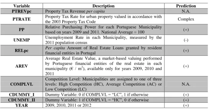
Table 1: Variable Definitions
Variable Description Prediction
PTREVpc Property Tax Revenue per capita N.A.
PTRATE Property Tax Rate for urban property valued in accordance with
the 2003 Property Tax Code Complex
PP Relative Purchasing Power for each Portuguese Municipality
based on years 2009 and 2011. National Average = 100 (+)
UNEMP Unemployment Rate in each Municipality, measured by the
2011 population census (-)
RELpc Per capita Amount of Real Estate Loans granted by resident
financial entities in Portugal (+)
AREV
Average Real Estate Value, a market-based valuing performed by Portuguese financial entities of the real estate in each municipality (€ / m2
), available only for years 2009, 2010 and 2011
(+)
COMPLVL
Competition Level: Municipalities are assigned to one of three levels: High Competition (HC), Average Competition (AC) or Low Competition (LC)
N.A.
CDUMMY_I Dummy Variable: 0 if COMPLVL = “LC”, 1 if otherwise (+)
CDUMMY_II Dummy Variable: 1 if COMPLVL = “HC”, 0 if otherwise (+)
YEAR 2009, 2010, 2011 or 2012 (+)
Whenever data is unavailable as a whole for a certain year for the control variables, we assume that the values in that year equal those of the previous year. Thus, we use the purchasing power values of 2009 and 2011 also for 2010 and 2012, respectively. Likewise, we use the average real estate values of 2011 for year 2012. For the unemployment figures, we rely always on the values of the 2011 census, as its figures are much more reliable and realistic than the unemployment estimates provided yearly.
13
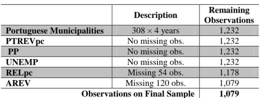
Some sporadic cases of missing data will place some minor restrictions on our sample. On Table 2 we present the restrictions that lead to the ultimate sample composition.
Table 2: Sample Formation
Description Remaining
Observations
Portuguese Municipalities 308 × 4 years 1,232
PTREVpc No missing obs. 1,232
PP No missing obs. 1,232
UNEMP No missing obs. 1,232
RELpc Missing 54 obs. 1,178
AREV Missing 120 obs. 1,079
Observations on Final Sample 1,079
The missing data for real estate valuing (AREV) and for the value of real estate loans per capita (RELpc) is not neglegible in number, but its impact is geographically restricted, as it is essentially due to missing data municipalities in the Autonomous Regions of Azores and Madeira. The restrictions due to missing RELpc and AREV data will not impact the models that will solely use tax rates to explain tax revenue. No instance of sporadic missing data exists for the tax revenue, purchasing power and unemployment figures.
4.3 Tax Rates
As mentioned on section 3, during the period of our sample two different tax rates could apply to real estate, depending on whether the property had been valued according to the rules of the 2003 Property Tax Code or not. This raises the question of which tax rate should be incorporated in our models, or whether both should be included, either through a kind of weighted variable taking into account both rates, or through the separte inclusion of the two Property Tax rates.
We believe there are strong reasons for taking into account only the tax rate for real estate valued under the 2003 rules. Indeed, as time went on, the rate for non-valued became progressively less relevant. This is even truer when discussing competition and competitive dynamics, as these are strictly related with new or transactioned properties, all of these having been valued according to the 2003 Property Tax Code.
This problem could potentially be solved by creating a true weighted tax rate, one that would weight both tax rates according to the proportion of property they apply to, idealistically at a municipal level. Since such information is not available, introducing a second, hardly relevant
14
rate – which became altogether irrelevant in 2013 – would risk introducing unnecessary distortion without any tangible benefit.
4.4 Competition Levels
Given that we wish to study the impact of competition of the Property Tax revenue, our analysis will be richer if we work with a heterogeneous sample, i.e. a sample that includes both municipalities in very competitive settings, either because they make part of a metropolis or because they compete in the international vacation home market; and municipalities where little to no competition exists, for example in poorer regions with high unemployment rates. Portugal, despite having a land area of only 35,603 square miles and a population of only approximately 10,5 million, is a country of deep economical and geographical contrasts, and is thus a prime sample for our purpose. Indeed, very strong asymmetries exist between the more economically developed Portuguese Atlantic coastline and the interior (Silva and Ribeiro, 2012; Morais and Fernandes, 2011).
In order to serve as a base for our tests on the impact of competition, we will divide our sample according to three competition levels: High Competition (HC), Average Competition (AC) and Low Competition (LC). We will assign municipalities en bloc according to the assignment given to their region, and we will draw on the statistical NUTS III administrative divisions for that purpose, with an exception for the Autonomous Regions of Azores and Madeira.
The municipalities of Grande Lisboa and Península de Setúbal, which form the Lisbon Metropolitan Area; of Grande Porto and Entre Douro e Vouga, which form the Greater Metropolitan Area of Porto; as well as of Algarve are classified as High Competition, a total of 48 municipalities. Lisbon and Porto are the two only Portuguese metropolises, and have experienced significant migratory fluxes between the municipalities of each metropolis, being a potential fertile ground for tax competition. The Algarve region is the most famous Portuguese touristic destination and one of the most important European touristic destinations, also being famous for being an attractive vacation home market and having a growing influx of foreign residents.
The remaining municipalities of the Portuguese Atlantic coastline – namely those of the Minho-Lima, Cávado, Ave, Tâmega, Baixo Vouga, Baixo Mondego, Pinhal Litoral, Oeste,
15
Médio Tejo, Alentejo Litoral and Lezíria do Tejo regions – are classified in the category Average Competition, as well as the municipalities of the archipelago of Madeira. While the classification of the former is intuitive, as the coastline municipalities are generally economically developed, have access to excellent infrastructures – including highways, railways and seaports – but remain clearly a level behind the Metropolitan Areas of Lisbon and Porto, the classification of Madeira in this category is a compromise between its unfavorable geographical position and its high degree of economic development, especially in what pertains to real estate14. The Average Competition group has thus a total of 113 municipalities.
The municipalities of interior Portugal, economically less developed, with persistent unemployment, with significant outgoing migration and with a less favorable geographical position, are classified with the label Low Competition. These are the municipalities in the NUTS III regions of Douro, Alto Trás-os-Montes, Pinhal Interior Norte, Dão-Lafões, Pinhal Interior Sul, Serra da Estrela, Beira Interior Norte, Beira Interior Sul, Cova da Beira, Alto Alentejo, Alentejo Central and Baixo Alentejo. We also include the Archipelago of Azores. A total of 147 municipalities are classified as Low Competition.
Table 3: Regions and Municipalities according to Competition Level
14 The categorization of Madeira can obviously change, and in order to correctly categorize this archipelago one
has to monitor the future evolution as the two main drivers (geographic conditionalisms and economic development). It should be particularly interesting to follow the economic impacts of the 2011 bail-out to the Madeira Regional Government.
Competition Level
(COMPLVL) NUTS III / Autonomous Regions
Number of Municipalities
High (HC) Grande Lisboa, Península de Setúbal, Grande Porto,
Entre Douro e Vouga 48
Average (AC)
Minho-Lima, Cávado, Ave, Tâmega, Baixo Vouga, Baixo Mondego, Pinhal Litoral, Oeste, Médio Tejo, Alentejo Litoral, Lezíria do Tejo, R.A. Madeira
113
Low (LC)
Douro, Alto Trás-os-Montes, Pinhal Interior Norte, Dão-Lafões, Pinhal Interior Sul, Serra da Estrela, Beira Interior Norte, Beira Interior Sul, Cova da Beira,
Alto Alentejo, Alentejo Central, Baixo Alentejo, R.A. Açores
16
4.5 Summary Statistics
We present summary statistics (number of observations, mean, median, standard deviation, maximum and minimum) for our main variables, which are displayed on Table 8 (Appendix A). These descriptive statistics show some consistent trends which are in accordance with the rationale that lead to the segmentation of regions (and their municipalities) according to distinct competitive levels.
Indeed, there is a consistent trend for more (less) competitive municipalities having higher (lower) averages for tax revenue, tax rates, purchasing power, unemployment, real estate loans per capita and average real estate value, i.e. for all variables. One can, however, envisage a surprise in relation to one of our predictions: unemployment is higher on average on more competitive municipalities, which also seem to have higher tax revenue on average. We will thus keep this variable under a special focus during our analysis.
We compute the correlation coefficients between the tax revenue and the explanatory variables, the results being displayed on Table 415, and we find significant positive correlation with all the explanatory variables, including unemployment, which goes against our prediction, as we had predicted a negative correlation.
The possibility of a positive correlation between unemployment and Property Tax revenue, despite not being the focus of our work, deserves at least a tentative explanation. Unemployment tends to be larger in urban centers, as in rural areas other options are available, like subsistence farming, and stronger informal social protection networks exist (e.g. family, vicinity ties). Also, since real estate is usually a long-term asset, it should not be influenced by short-term or recent unemployment, and a more structured analysis of unemployment would be necessary, one that would, for example, analyze historical unemployment rates and the timings of real estate investment decisions.
15 In all our tables, *, ** and *** indicate statistical significance at 10%, 5% and 1%, respectively. All our
17
Table 4: Correlation Statistics
PTREVpc Total LC AC HC PTRATE 0.41 *** 0.55 *** 0.44 *** 0.10 n.s. PP 0.56 *** 0.56 *** 0.70 *** 0.09 n.s. UNEMP 0.18 *** 0.03 *** -0.18 *** 0.29 *** RELpc 0.46 *** 0.39 *** 0.38 *** 0.22 *** AREV 0.71 *** 0.12 *** 0.47 *** 0.69 *** YEAR 0.10 *** 0.20 *** 0.14 ** 0.12 n.s.
18
5. THE LAFFER CURVE AND THE DETERMINANTS OF PROPERTY TAX REVENUE
5.1 Testing the Laffer Hypothesis
Our first goal is to test whether the Laffer hypothesis holds for Property Tax in our sample. However, in order to do so, we will begin by testing the following model type which does not recognize the Laffer hypothesis:
(5.1) Here, like in all the following models, “i” corresponds to each of the Portuguese municipalities and “t” corresponds to years 2009, 2010, 2011 or 2012.
The structure of this type of model does not take into account the Laffer effect, as it has a single and linear coefficient (β1) that relates tax rates (PTRATE) to per capita tax revenue (PTREVpc), that is, it assumes that increasing tax rates are correlated with increasing – because one predicts the coefficient to be positive – tax revenue.
Before advancing further, a brief discussion on heteroskedasticy must be made. A simple graphical and statistical analysis of the distribution of the per capita tax revenue according to the different tax rates clearly shows the presence of heteroskedasticity in the sample, the variance being much higher on the extreme rates, i.e. around the minimum and maximum legal rates. We run the White’s Test for testing the presence of heteroskedastacity, which confirms the rejection of the null hypothesis, i.e. we reject the hypothesis of homoskedasticity.
We will thus use the Ordinary Least Squares (OLS) estimation, applying the White’s Correction in order to address the presence of heteroskedasticity. In order to strengthen our results, we will make a second estimation using Weighted Least Squares (WLS), where we will use a weight based on the real estate value (AREV), namely its inverse variance. We will, for each regression aimed at explaining tax revenue, use this second estimation method in order to improve the robustness of our results, unless stated otherwise.
19
As we have mentioned, the regressions based on Equation 5.1 do not take into account – indeed its formal expression contradicts or at least ignores – the Laffer effect, whereby from a certain point an increase of the tax rate may lead to lower tax revenue. The classical representation of the Laffer curve is a concave (on the most schematic representation, a parabolic) curve, which may be represented by a second order equation. Consequently, we adapt our model in order to take into account the Laffer effect.
(5.2) In order to form a classical Laffer peak, the coefficient β1a should be positive and the coefficient β1b should be negative. The introduction of the new variable is to be tested by comparing the restrained model (expressed in Equation 5.1) to the unrestrained model (expressed in Equation 5.2), applying the redundant variables test as to discern whether the introduction of new variables produces a statistically significant improvement. Such test evaluates whether incorporating a mechanism that allows for Laffer effect expressed on its classical form improves the model or not. This procedure and its rationale will be repeated in the following section.
5.2 The Laffer Curve Shape Controversies
The controversies around the possible shapes of the Laffer curve are old and play a preeminent role in Laffer literature. A hypothesis suggested by Spiegel and Templeman (2004) is particularly relevant to our present study: in a very strong-worded article, they claim to “debunk” the traditional concave curve with one peak which represents the traditional form of the Laffer curve, and suggest a curve with at least two peakes.
We will take into consideration this possibility, by running regressions with the structure of the equation below. Indeed, a fourth-order equation where the coefficients for the second and forth order variables are negative and the first and third variable coefficients are positive may form a two-peaked curve, thus reflecting the theory advanced by Spiegel and Templeman (2004).
20
(5.3) As in the previous models, we will run this equation using both OLS with the White’s Correction for heteroskedascity and WLS; and test whether any improvement was made by the introductions of the second, third and fourth-degree terms.
5.3 The Laffer Curve through Rate-Revenue Models
A possible objection to the models that we have been presenting is that the Laffer effect must be analyzed by studying the direct relationship between tax rate and tax revenue, with no additional variables: after all, the Laffer curve is a graphical expression of that relation, and nothing more. Therefore, is it correct to mix the sole and only (direct) explanatory variable of the Laffer curve with other variables which are foreign to the model?
Yes and no. We do not intend to introduce new explanatory variables on the Laffer curve, but rather to actually perform a “reality check” to the Laffer effect. We do recognize that part of the Laffer effect may – and indeed should – be contained in other variables that indirectly affect the Laffer curve and that have here been placed side by side with the direct Laffer curve’s sole explanatory variable – i.e. tax rate. However, that is necessary in order to discern the effect that tax rates exercise per se.
However, it does make sense to express our findings in a Laffer-like setting, i.e. using tax rates as the only explanatory variables, not only due to the conceptual objection we have just discussed, but such a step seems necessary also in order to gain further insights about the shape of the Laffer curve, and even useful to assess its existence.
For that purpose, we will present, for each regression, a reduced version of the model containing only tax rates as explanatory variables, to which we call “rate-revenue”. We will often refer to the effects of competition on the rate-revenue model, as it is a broader concept than the Laffer curve, the later being a subset of the former, having also the advantage of raising no a priori biases, being an expression void of political and ideological connotations.
21 (5.4) (5.5) (5.6) 5.4 Estimation Results
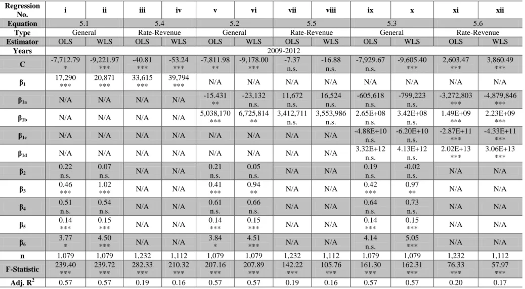
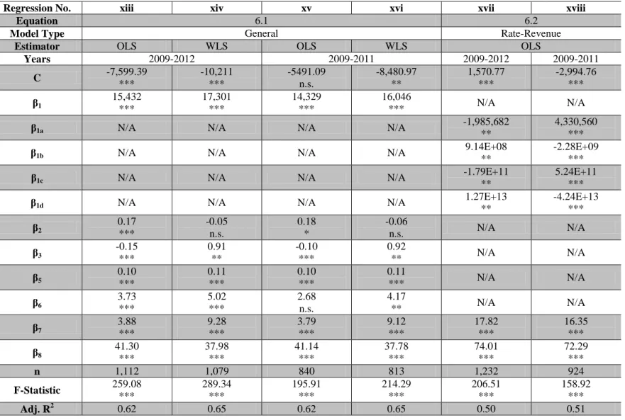
The six equations that we have presented thus unfurl at two regressions each, in a total of twelve models. Indeed, for each equation we use both the OLS (with the White’s Correction) and WLS estimators. Regressions i-iv hold a non-Laffer relationship between tax rate and tax revenue; regressions v-viii are designed to allow for a single-peaked curve; regressions ix-xii allow for a two-peaked curve. The results are presented on Table 5.
22
Table 5: Results for Models i-xii
Regression
No. i ii iii iv v vi vii viii ix x xi xii
Equation 5.1 5.4 5.2 5.5 5.3 5.6
Type General Rate-Revenue General Rate-Revenue General Rate-Revenue
Estimator OLS WLS OLS WLS OLS WLS OLS WLS OLS WLS OLS WLS
Years 2009-2012 C -7,712.79 * -9,221.97 *** -40.81 *** -53.24 *** -7,811.98 ** -9,178.00 *** -7.37 n.s. -16.88 n.s. -7,929.67 n.s. -9,605.40 *** 2,603.47 *** 3,860.49 ***
β1 17,290 *** 20,871 *** 33,615 *** 39,794 *** N/A N/A N/A N/A N/A N/A N/A N/A
β1a N/A N/A N/A N/A -15.431
** -23,132 n.s. 11,672 n.s. 16,524 n.s. -605,618 n.s. -799,223 n.s. -3,272,803 *** -4,879,846 ***
β1b N/A N/A N/A N/A 5,038,170
*** 6,725,814 ** 3,412,711 n.s. 3,553,986 n.s. 2.65E+08 n.s. 3.42E+08 n.s. 1.49E+09 *** 2.23E+09 ***
β1c N/A N/A N/A N/A N/A N/A N/A N/A -4.88E+10
n.s. -6.20E+10 n.s. -2.87E+11 *** -4.33E+11 ***
β1d N/A N/A N/A N/A N/A N/A N/A N/A 3.32E+12
n.s. 4.13E+12 n.s. 2.02E+13 *** 3.06E+13 *** β2 0.22 n.s. 0.07 n.s. N/A N/A 0.21 n.s. 0.05 n.s. N/A N/A 0.19 n.s. -0.02 n.s. N/A N/A β3 0.46 *** 1.02 *** N/A N/A 0.41 *** 0.94 ** N/A N/A 0.42 *** 0.97 ** N/A N/A β4 0.51 n.s. 0.54 n.s. N/A N/A 0.61 n.s. 0.66 n.s. N/A N/A 0.64 n.s. 0.73 n.s. N/A N/A β5 0.14 *** 0.15 *** N/A N/A 0.14 *** 0.15 *** N/A N/A 0.14 *** 0.15 *** N/A N/A β6 3.77 * 4.50 *** N/A N/A 3.84 * 4.51 *** N/A N/A 4.14 n.s. 5.05 *** N/A N/A n 1,079 1,079 1,232 1,112 1,079 1,079 1,232 1,112 1,079 1,079 1,232 1,112 F-Statistic 239.40 *** 239.72 *** 282.33 *** 210.32 *** 207.16 *** 207.89 *** 142.22 *** 105.76 *** 161.30 *** 162.31 *** 76.33 *** 57.97 *** Adj. R2 0.57 0.57 0.19 0.16 0.57 0.57 0.19 0.16 0.57 0.57 0.20 0.17
23
All control variables have the expected signs, with the exception of unemployment, a surprise which had already been foreseen in the correlation analysis, a result for which we had also advanced and discussed a possible explanation.
In what regards the general model, the regressions i and ii show unequivocally that it is significant, both converging to a high adjusted-R2 value of 0.57. This first result is highly important, not only due to the potential practical applications of a model that can explain Property Tax revenue with few and easy to obtain inputs, but also because it allows us to continue with our research on the impact of competition on tax revenue.
Before continuing our endeavor, two structural questions must be addressed and settled: First, should all the variables remain in the model, i.e. could we improve the model by removing statistically insignificant or doubtfully-significant variables? Second, what kind of tax-revenue/tax-rate relationship should be incorporated into the model?
Regarding the first question, all control variables seem to be significant, with two exceptions: purchasing power and the value of real estate loans per capita. This result is somewhat surprising, but may be explained by the fact that the average real estate value variable can capture much more efficaciously the income and economic drivers that Purchasing Power attempted to address, and the RELpc variable is likely to contribute to the capture of these same drivers. However, since the AREV and RELpc variables are arguably less common than purchasing power, on Appendix B we will re-estimate the model substituting AREV and RELpc for purchasing power, so as to provide an alternative model using a single and more commonly available variable.
A similar question concerns the presence of the Laffer effect and the significance of the variables added in order to potentially express it. A first analysis shows that the introduction of the second third and fourth order expressions for the Property Tax does not seem promising for the general type models.
Indeed, as for the inclusion of PTRATE2, i.e., as whether on models v and vi were an improvement vis-à-vis models i and ii, no further analysis is necessary. On model vi the variable is not significant when α = 1% and PTRATE becomes non-significant; and, on model v, the PTRATE variable is not significant when α = 1%. The addition of these variables does
24
not produce any improvement on the overall significance and power of the model, the F-Statistics being reduced and the adjusted-R2’s remaining both at 0.57.
The analysis for the joint inclusion of PTRATE2, PTRATE3 and PTRATE4 is even more straightforward: all the tax rate variables become non-significant on models ix and x, the models’ F-Statistic’s are reduced and the adjusted-R2’s do not improve.
These tests show that a model based on a linear relationship between Property Tax revenue and Property Tax rate is the most adequate, according to our sample. Having settled the structure for the general model, we can now address properly the question raised by the unconvincing results for the purchasing power and real estate loans per capita variables. Does it mean we must dismiss both variables from our final general model? Not necessarily. Indeed, the removal of the less significant of these two variables (RELpc) immediately renders the PP variable unmistakably significant using the OLS estimator (cf. regression xiii, Table 6). However, when using the WLS estimator, purchasing power remains at best doubtfully significant.
We therefore define a new equation, similar to Equation 5.1 but without the Real Estate Loans per capita variable. This equation will serve as a general model basis for our studies on the effects of competition on the following section, notwithstanding the rate-revenue model which we will discuss below.
(5.7)
The results of the rate-revenue models are complex, interesting and deserve a paused analysis. The coefficients of the models designed to allow a classical Laffer curve do not point to the formation of such a curve, as a simple graphical analysis shows. These coefficients are moreover clearly non-significant on both model vii and model viii.
25
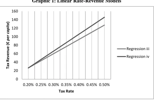
Graphic 1: Linear Rate-Revenue Models
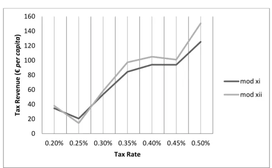
Graphic 2: Quadratic Rate-Revenue Models
However, the results for models xi and xii are not only robust, but, as Graphic 3 shows, seem to indicate some limited presence of the Laffer effect with a multiple-peaked Laffer Curve, two peaks being visible in the graphic and an hypothetical third peak that may or may not exist16 if the tax rate were greater than 0.5%. We conduct the redundant variables Test that confirms that the inclusion of variables PTRATE2, PTRATE3, and PTRATE4 is not redundant and improves the model, as one could already predict by the regression results, as the
16 A purely mathematical extension of the curve would not point to a third peak, but the outright extrapolation of
these results for outside the original range would be a methodological mistake. 0 20 40 60 80 100 120 140 160 0.20% 0.25% 0.30% 0.35% 0.40% 0.45% 0.50% Tax R e ve n u e ( € pe r capita ) Tax Rate Regression iii Regression iv 0 20 40 60 80 100 120 140 160 0.20% 0.25% 0.30% 0.35% 0.40% 0.45% 0.50% Tax R e ve n u e ( € pe r capita ) Tax Rate Regression vii Regression viii
26
introduced variables were significant and the values for the adjusted-R2’s improved, even if only slightly, from 0.19 and 0.16 (regressions iii and iv) to 0.20 and 0.17 (regressions xi and xii).
Graphic 3: Fourth-Degree Rate-Revenue Models
If the results from the general models seem to point to a positive linear correlation between the tax rate and tax revenue, and if the Laffer-effect visible in the rate-revenue models is limited, at best, can we affirm the presence of a Laffer curve at all? In order to address this question, some points must be made that may help us gaining a better understanding of what we can or cannot find in the present study.
First, the range of possible tax rates in this particular tax is quite restricted by national-level legislation, and these rates, even at their maximum level, are far from what we could consider confiscatory or even prohibitive levels. Obviously, one must keep in mind that although the rates are nominally low, the tax bases are usually high values (values of real estate property). Nevertheless, the range is limited and has a relatively low ceiling, which makes it very likely that, if the Property Tax revenue follows a Laffer curve pattern, we be still away from its prohibitive area.
Second, the Laffer effect is subtle, and tends to remain so until very high tax rates are achieved, which is when this effect may appear clearly with devastating consequences. It remains relatively “hidden” when discussing low-to-moderate tax rates.
0 20 40 60 80 100 120 140 160 0.20% 0.25% 0.30% 0.35% 0.40% 0.45% 0.50% Tax R e ve n u e ( € pe r capita ) Tax Rate mod xi mod xii
27
It is not surprising then that, in such a context and when mixed with much “stronger” variables – the market-driven value estimates for real property (AREV), for example –, the Laffer effect cannot be a major driver, and, in an overall analysis, may remain unnoticed, at least until the prohibitive threshold is reached.
What the rate-revenue model can and seem to indicate at this point is that, albeit subtly, there is evidence of a manifestation of the Laffer effect in our sample, whose meaning we will discuss in detail in our conclusions.
28
6. THE COMPETITION EFFECT AND THE LAFFER CURVE
6.1 The Quest for the Competition Effect
In this section, we will seek to identify the potential effects of competition on the Laffer curve and, on more broad terms, on our models, through two complementary analyses.
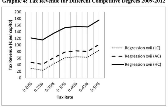
The first analysis, represented on Equations 6.1 and 6.2, relies on dummies that control for the levels of competition that we have assigned to each municipality; the second, which we will apply solely to the rate-revenue models – and expressed on Equation 6.3 – is simply a partitioning of the sample according to the competition levels, in order to draw and compare different tax rate-revenue curves for the different competition levels.
The scope of the two analyses should not be confused. While the first is intended to confirm whether there is a (positive) overall correlation between competition and tax revenue – and, if this should be the case, the result on the rate-revenue model would be a simple shift upwards –; the second analysis is broader, and is indeed one of the core aspects of our study: how do rate-revenue curves vary according to the degree of competition? How do they compare with each other? Thus, although both have different purposes and meanings, the second analysis is, in its implications for the Laffer curve, more wide-ranging and potentially more impacting.
(6.1) A simplified version of Equation 6.1 that does not include AREV as an explanatory variable is presented and discussed on Appendix B.
(6.2) (6.3)
29
On Equation 6.3, “c” represents the competitive level (Low, Average or High) of each municipality17.
For the first analysis we will use, like we have done previously in order to obtain greater robustness, two estimators: OLS with White’s correction; and WLS with inverse variance, this time based on the RELpc variable serving as weight. The choice of this variable has a similar rationale to AREV, but since the former is no longer an explanatory variable, its adoption as weight seems methodologically more correct at this point. For the second analysis, and given that the weight used on the WLS estimator – in this case, RELpc – could place a significant restriction18 on the sub-samples, we will employ solely the OLS estimator.
6.2 An Earthquake, Two Mountains?
When focusing on the effects of competition on the tax rate-revenue relation and trying to discern the shape of the tax rate-revenue curves for each degree of competition, we should mind the possible effects of an “earthquake” which affects our sample and may influence our results, particularly in this analysis. This metaphorical earthquake is the already mentioned change of tax range for year 2012, the minimum / maximum rates changing from 0.2% / 0.4% to 0.3% / 0.5%.
Can this “earthquake” change our landscape and shape two different “mountains”, i.e. two different tax rate-revenue curves? In what way does it affect our models?
The question is indeed especially relevant for our discussion, since a tax rate can have very different meanings depending on whether it was freely and strategically adopted or whether it was imposed by a third-party. For example, a 0.3% tax rate has a radically different meaning if adopted by a municipality before 2012 – it was exactly the “central” rate in the 0.2% / 0.4% range – or during 2012, where the 0.3% rate became the minimum imposed by national legislation.
In our estimations we will thus always consider two different time-frames: one encompassing all the timeframe of our sample, the other limited to 2009-2011, before the shift in the tax rates range. The results arising from the second timeframe can be seen as more reliable, being fruit of a sample established on a common basis, and thus more robust.
17 Not to be confused with “1c”, the identifier for PTRATE3 in our fourth-degree equations. 18
30
6.3 Estimation Results
On Table 6 we present the results for the estimation, performed through both OLS and WLS estimators, of Equations 6.1 and 6.2 using our sample, in order to analyze the impact of the dummies (CDUMMY_I and CDUMMY_II) that incorporate the three distinct competitive levels on the models, i.e. to assess whether competition has a statistically significant impact on tax revenue. We present results both for the total period of the sample, 2009-2012, and for the period 2009-2011 (cf. section 6.2).