http://dx.doi.org/10.1590/S1982-21702015000300027
Artigo
TWO-EPOCH OPTIMAL DESIGN OF DISPLACEMENT MONITORING
NETWORKS
Monitoramento de deslocamento de redes baseado em método de otimização por duas épocas
Mehdi Eshagh1, 2
Mohammad Amin Alizadeh-Khameneh2
1Department of Engineering Science, University West, Trollhättan Sweden
2Division of Geodesy and Satellite Positioning, Royal Institute of Technology (KTH), Stockholm, Sweden
Emails: [email protected]; [email protected]
Abstract:
In the traditional method of optimal design of displacement monitoring networks a higher
precision, √ times better than the desired accuracy of displacements, is considered for the net
points in such a way that the accuracy of the detected displacements meets the desired one. However, in this paper, we develop an alternative method by considering the total number of observations in two epochs without such a simple assumption and we call it two-epoch optimisation. This method is developed based on the Gauss-Helmert adjustment model and the variances of the observations are estimated instead of the weights to optimise the observation plan. This method can deliver the same results as the traditional one, but with less required observations in each epoch.
Keywords: Gauss-Helmert Model; Least-Squares; Optimal Variance; Precision of Displacements.
Resumo:
Nos métodos tradicionais de monitoramento de deslocamento de redes é exigida alta precisão dos pontos que compõem a rede, em torno de √ vezes a precisão requerida, de forma que a precisão exigida no projeto seja alcançada. Neste artigo foi desenvolvido um método alternativo que considera o número total de observações obtidas em duas épocas, sendo chamado de otimização em duas épocas. Este método foi desenvolvido baseado no modelo de ajustamento de Gauss-Helmert e ao invés dos pesos são estimadas as variâncias das observações para otimizar o modelo de observação. Este método pode ter resultados iguais ao método tradicional, mas com menor quantidade de observações requeridas em cada época.
1. Introduction
The geodetic networks are designed for different purposes, but one of the most important applications of such networks is to monitor deformation of man-made structures or the Earth. Amongst numerous studies about the design of such networks, we mention the work done by Kuang (1991). Blewitt (2000) and Gerasimenko et al. (2000) studied the design problem of a monitoring network based on the geophysical parameters and fault-mechanics and Yetki et al. (2008) studied a numerical algorithm of particle swarm optimisation for a similar purpose.
Generally, an optimal geodetic network is a network having high precision and reliability designed according to economic considerations. The precision of the network is related to the estimated errors of the coordinates of the net points and the reliability is the resistance of the network to the possible gross errors. The first step of the geodetic network design is so-called the zero-order design (ZOD) in which the best datum of the network is defined as it affects the precision of the network. Different criteria exist for the ZOD. Teunissen (1985) presented the ZOD according to the theory of generalised matrix inverses and its relations with datum and rank deficiency of the design matrix. Kuang (1996) presented different criteria for the ZOD, and Eshagh (2005) suggested the minimum norm and trace of the co-factor matrix as the best criteria for datum definition. There are three well-known ways to find the best configuration of networks, i.e., the first-order design (FOD). One can use the trial and error, the analytical or metaheuristic approaches. Here, we just explain the first two methods, and the reader is referred to Berné and Baselga (2004) for the metaheuristic method. In the former, the objective function (OF) is computed with a proposed solution for the problem. If the suggested solution does not satisfy the OF, the solution is changed and the OF is computed again. This process is repeated until the requirement is satisfied. The analytical approaches take advantage of a mathematical algorithm and design the network in such a way that the quality requirement of the network is satisfied. A pioneer in using optimisation theory for the FOD purpose was Koch (1982) and Koch (1985) who used the quadratic programming theory (Bazaraa and Shetty 1979) to optimise the configuration of a network. Kuang (1991), Kuang (1996) and Amiri-Simkooei (1998) studied this issue further and considered different types of optimisation methods. Berné and Baselga (2004) used the simulated annealing method for the FOD. Amiri-Simkooei (2008) presented an analytical approach for the same purpose.
Grafarend (1975), Schmitt (1980) and Schmitt (1985) presented different approaches to the second-order design (SOD) where the observable weights and type are determined. Xu (1989) developed a multi-objective optimisation model (MOOM) for the SOD purpose and Kuang (1993) presented another approach to the SOD leading to maximum reliability using linear programming (see e.g. Bazaraa 1974, Smith et al. 1983). Amiri-Simkooei (2004) presented a new method for the SOD. Doma (2014) developed another method for the SOD and compared it
with Kuang’s (1996) method and concluded the both of them can meet the precision criterion of
the strain parameters.
criterion exists in the OF, it is called single-objective optimisation model (SOOM); if two criteria exist, it is a bi-objective optimisation model (BOOM) (Mehrabi 2002), and, if we have more than two criteria, we call it MOOM (Xu 1989). A simple comparison between different SOOMs has been carried out in Eshagh and Kiamehr (2007). This comparison shows that reliability is a much better criterion than the precision criterion in SOOMs. The capability of the BOOM versus SOOM was presented in Eshagh (2005). Bagherbandi et al. (2009) compared SOOM and MOOM in a simulated geodetic network and concluded the superiority of the MOOM with respect to SOOM. Alzubaidy et al. (2012) discussed the problem of the FOD and SOD in a micro-geodetic network. Amiri-Simkooei et al. (2012) presented some basic concepts related to the optimisation and design of geodetic networks. Eshagh and Alizadeh-Khameneh (2014) concluded that in the case of using a BOOM of precision and reliability, constraining the OF to the precision and reliability constraints are not necessary.
In the optimal design of a monitoring network, the accuracies of the displacements and/or deformation parameters are also considered as some criteria. Displacements are important for monitoring networks as the deformation parameters are estimated from them, if the monitored object can be considered as a continuum medium. However, not all objects are of continuum nature, in such a case displacements in different parts of the object are considered instead of deformation parameters. So far, geodetic networks have been designed based on the precision and/or reliability of the network for one epoch of observations. In fact, in displacement monitoring networks the goal is to determine the displacements or the coordinate differences between two epochs of observations. Considering two epochs for optimising a displacement monitoring network is a new issue, which is studied for the first time and we will discuss in this study based on the precision of the estimated displacements. Here, we will discuss both methods of one-epoch and two-epoch optimisation and compare them in theoretical and practical view.
2. One-epoch optimisation
In optimisation and design of geodetic networks usually one epoch for measuring the necessary data is considered. However, if our goal is to determine the displacements, optimal design of a network by considering one epoch of observation is not fully correct. In the past, for designing monitoring networks, the quality of the observables has been assumed to be the same (Kuang 1996, p. 302). Also, a similar configuration for the networks was assumed for all epochs of measurements. However, the configuration and number of data in one epoch can be different from another meanwhile preserving the precision of the displacements. In the following, we will explain the traditional method for optimal design of a monitoring network mathematically and we call this method one-epoch optimisation.
Let the following Gauss-Markov model for least-squares adjustment of geodetic networks at the epoch i:
where A stands for the design matrix, xk the vector of unknown coordinates, Lk the vector of
As can be seen in Equation 1, the design matrix remains the same in any epoch of k but the observation vector will change from one epoch to another and correspondingly their errors. The result of any change in the observation vector leads to changes in the coordinates of the points, which are recognised as displacements. However, some statistical tests should be performed to see if the displacements are meaningful and the observation changes are not due to the non-random errors (see e.g. Kuang 1996, p. 274-275). If we consider two epochs of 1 and 2 and subtract the organised Gauss-Markov model of Epoch 2 from that of 1, we have:
where ΔL is the difference of the vector of observations in both epochs and Δε their corresponding errors. The least-squares solution of the displacements Δx is:
where
where D is the datum matrix and P is the weight matrix of both epochs. In fact, the above least-squares solution is the results of minimising the following OF:
The variance-covariance (VC) matrix of the estimated displacements ∆�̂ is:
where H is the matrix, which spans the null space of the design matrix A, and usually used for adjustment of the network by the inner constraints method; also E = HTDDTH.
In the case that the same observables with the same qualities are observed in the network, the matrix P will be:
Therefore, Equation 6 will change to:
This means that the errors of the optimised network should be considered √ times smaller than
what we expect for an ordinary network, if the network is going to be used for displacement monitoring (Kuang 1996, p. 302). Let us consider a two-dimensional network for implying our mathematical presentation, but we emphasise that what we present for such a network will be valid for any type of displacement monitoring network. Now, if �∆� ̂ is expanded by the Taylor series we have:
and
�∆� ̂0 is the initial VC matrix of the displacements in the present status; Δxi and Δyi are the position or configuration changes, and Δpj is the weight updates of the observations. In fact, by changing the configuration using Δxi and Δyi; and observational plan by Δpj, we fit �∆� ̂0 to the desired criterion matrix, C
2 in a least-squares sense. Note that we divide the matrix C by 2 to
emphasise that the desired errors of the points are √ times smaller than the errors of displacements. To do so, we can write Equation 9 in the following matrix form:
where
T is constructed as a × × + matrix, and the vectors w and u have the
dimensions of + × and × × , respectively.
In order to derive w, the following optimisation model should be solved:
subject to
where
2
where [a1i,a2i] and [b1i,b2i] are the boundary values of the unknown coordinate changes, Δxi, Δyi , and i=1,...,m. For the weight improvements Δpj, j=1,...,n are introduced and �0, j=1,...,n are the approximate weights for pj. Note that the coordinate changes, Δxi and Δyi, are the changes in the network configuration and not the displacements.
All of these processes are done for designing a displacement monitoring network based on the traditional one-epoch optimisation. In fact, it is an ordinary network optimisation but only the criterion matrix is divided by 2; for more details see Kuang (1991) and Kuang (1996).
3. Two-epoch optimisation
The problem with one-epoch optimisation is that we cannot directly consider the observations of two epochs, and the optimisation is just done based on one epoch with those observations, which are not really observations, but the observation differences in two epochs. This is the restriction due to the use of Gauss-Markov model. Now, we use another mathematical model, which can consider all of the observations in two epochs, i.e. the Gauss-Helmert adjustment model. In this case, instead of Equation 2, we can write:
The least-squares solution of Equation 20 is:
where
and the VC matrix of the displacement is:
In fact, the solutions (3) and (21) are identical, where the former equation is derived based on the Gauss-Markov adjustment model, which is a particular case of the Gauss-Helmert adjustment models. Another problem of the one-epoch optimisation is that when one observable has an insignificant influence in the precision of network in Epoch 1, the corresponding one is also insignificant in Epoch 2. However, by using the Gauss-Helmert model we can separate the observation sets from each other, but mathematically connect them by the matrix B. In this case, we have two sets of observations from two epochs preserving the accuracies of the detected displacements. Now, if we expand �∆� ̂, Equation 23, by the Taylor series, we have:
where ��∆�̂
� and
��∆�̂
� are defined in Equations 10 and 11, respectively and
��∆�̂
�� can be written
where qj are the diagonal elements of �∆� ̂ or the variances of observations.
It is of vital importance to note that j ranges from 1 to 2n, which means that when � ≤ , qj belongs to the observations of Epoch 1 and when j > n, to those of Epoch 2.
The difference between Equation 24 and Equation 9 is related to their last terms. In Equation 9, the derivative of �∆� ̂is taken with respect to the weight of observations whilst in Equation 24 with respect to their variances. Since we want to define a weight matrix, as we used in the Gauss-Markov model, we have to consider the addition of the VC matrices of both sets of observations and multiply them by B and BT. Therefore, we have to take the derivatives with respect to qj instead of pj, where qj =1/ pj. In this case, the total number of observations will be 2n for Equation 24, i.e. the total number of observations in both epochs. Equation 24 can be presented by the following matrix form:
where
The matrix T' and the vector W' have the dimensions of × × + and +
× , respectively, while the dimension of vector u' is the same as previous. Similar to Equation 17, an optimisation model can be formulated as:
subject to Equation 18 in which the elements of matrix b00 are written as:
4. Numerical studies
In order to test the presented theory for two-epoch optimisation, a simple trilateration network consisting of 7 net points and initially 21 length observations is designed and optimised for the purpose of displacement monitoring. At the first step, the one-epoch optimisation method is used. Here, we assume that the error of the displacements should be about 3 mm. In one-epoch optimisation we consider the error of each point smaller by √ so that after using the error propagation law of the random errors, it will be √ times larger for the displacements. In other
words, 3 is divided by √ meaning that the error of coordinates of each point should be 2.1 mm.
However, in two-epoch optimisation 3 mm is directly considered as the desired precision of the displacements.
Here, we use the optimisation toolbox of MATLAB® for our purpose and we assume that the position of the points can change not more than 2 metres. Also, we have found that to achieve high accuracy of the net points, Point 4 should be kept fixed as well as its direction towards Point 1 to define a proper datum, i.e. the minimum constraints. At the first step, all possible distances are considered, and in optimisation we try to delete some of them from the plan according to the desired accuracies of the displacements and by changing the configuration.
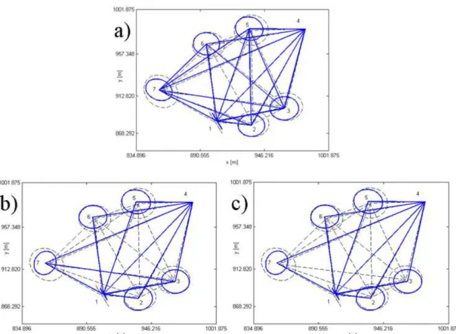
Figure 1a shows the optimised network by the one-epoch method on the background of the network prior to optimisation. As it is seen, the lengths L26, L32 and L 56 have been deleted from the observation plan, which means that the network is able to deliver displacement with the desired accuracy based on one-epoch method with 3 observations less than the planed one. All error ellipses of the displacements have been presented 5000 times larger than their true values for a better visualisation. They became larger after optimisation, which means that a precision of 3 mm for the displacement is achievable with 3 less observations.
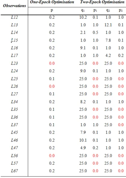
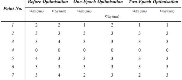
Figures 1b and 1c show the optimised network based on the two-epoch method. The former presents the optimised one in Epoch 1 and the latter in Epoch 2. In the one-epoch optimisation,
we considered a higher precision for the displacements by dividing the desired precession by √ ,
but in the two-epoch optimisation we do not have to do that as we can consider the observation plans of both epochs together and optimise them simultaneously. Lots of observations have been removed from the plan in the two-epoch optimisation. Also, we observe that the plan in Epoch 2 has one observation less than that in Epoch 1. This means that measuring the same quantity as those in Epoch 1 is not necessary. The figure shows that in order to attain the accuracy of 3 mm for the displacement at each point, observing two lengths from the reference points is sufficient.
Figure 1: Network configuration and error ellipses of the displacements before and after optimisation. a) Optimised network based on one-epoch optimisation, b) and c) two-epoch
optimisation of network in Epochs 1 and 2, respectively.
Table 1 presents the observation plan after one-epoch and two-epoch optimisations. L23, L26 and L56 are the observations to be deleted from the plan based on the former approach. In the latter, the variances of the observations are estimated instead of their weights. We assume a variance of 1 mm2 to avoid delivering zero variances for the observations and a maximum
variance of 25 mm2 (as the inverse of the smallest weight value from one-epoch approach, which
is rounded to zero in Table 1)as the criterion for deleting unnecessary observations. q1 and p1 are
the variance and the corresponding weight in Epoch 1 and q2 and p2 are the corresponding ones in
Table 1: Observation weights after network optimisation by two approaches, q1 and p1 are the
variance and weight in Epoch 1, and q2 and p2 contain the same definition in Epoch 2.
Table 2: Displacement error of net points before and after optimisation.
Finally, Table 3 illustrates that the position changes of the net points and the configuration of the optimised network are the same in both approaches as expected.
Table 3: Position changes after optimisation procedure, [m].
5. Conclusion
one-epoch method. The configuration and position changes of the points are the same in both approaches. In short, one- and two-epoch approaches both delivers similar accuracies of displacements and configuration, but the latter uses less observations in each epoch. Therefore, the two-epoch approach is more economical and practicable than the traditional one. One point that should be stated here is that the weight of one observation may come out considerably larger/smaller in one epoch than another. However, this point will not be significant if we consider the larger weight for that observation in both epochs. The important issue is the deletion of insignificant observations, which is done successfully in our approach. Since the observations of a displacement monitoring networking should be repeatedly measured, it is recommended that the two-epoch optimal design is performed just for the first two epochs. Later on, the same principle can be applied for designing an optimal observation plan for the subsequent epochs.
ACKNOWLEDGMENTS
The authors are thankful to Professor Lars E. Sjöberg at Royal Institute of Technology (KTH) and FORMAS for the financial support of the project DNR-245-2012-356.
REFERENCES
Alzubaidy, R. Z, H. A Mahdi, and Hanooka, H. S . “Optimized Zero and First Order Design of
Micro Geodetic Networks.” Journal of Engineering 18, no. 12 (2012): 1344-1364.
Amiri-Simkooei, Alireza. “A New Method for Second-order Design of Geodetic Networks:
Aiming at High Reliability.” Survey Review 37, no. 293 (2004): 552-560.
Amiri-Simkooei, Alireza. “Analytical First-order Design of Geodetic Networks.” Iranian
Journal of Engineering Sciences 1, no. 1 (2008): 1-12.
Amiri-Simkooei, Alireza. Analytical Methods in Optimization and Design of Geodetic Networks.
Surveying Engineering, Tehran: K. N. Toosi University of Technology, 1998.
Amiri-Simkooei, Alireza. “Comparison of Reliability and Geometrical Strength Criteria in
Geodetic Networks.” Journal of Geodesy 75, no. 4 (2001a): 227-233.
Amiri-Simkooei, Alireza. “Strategy for Designing Geodetic Network with High Reliability and
Geometrical Strength Criteria.” Journal of Surveying Engineering 127, no. 3 (2001b): 104-117.
Amiri-Simkooei, Alireza, J Asgari, F Zangeneh-Nejad, and Zaminpardaz, S . “Basic Concepts of
Optimization and Design of Geodetic Networks.” Journal of Surveying Engineering 138, no. 4
(2012): 172-183.
Bagherbandi, Mohammad, Mehdi Eshagh, and Sjöberg, Lars Erik . “Multi-Objective versus
Single-Objective Models in Geodetic Network Optimization.” Nordic Journal of Surveying and
Real Estate Research 6, no. 1 (2009): 7-20.
Bazaraa, Mokhtar Sadek, and Shetty, C. M . Nonlinear Programming. New York: John Wiley & Sons, Inc, 1979.
Berne, J. L, and Baselga, S . “First-order Design of Geodetic Networks Using the Simulated
Annealing Method.” Journal of Geodesy 78 (2004): 47-54.
Blewitt, G. “Geodetic Network Optimization for Geophysical Parameters.” Geophysical
Research Letters 22, no. 27 (2000): 2615-3618.
Doma, Mohamed Ismail Ali. “A Comparison of Two Different Measures of Precision into
Geodetic Deformation Monitoring Networks.” Arabian Journal of Science & Engineering 39
(2014): 695-704.
Eshagh, Mehdi. Optimization and Design of Geodetic Networks. Tehran: Islamic Azad
University, Shahr-e-Rey branch, 2005.
Eshagh, Mehdi, and Mohammad Amin Alizadeh-Khameneh. “The Effect of Constraints on Bi
-Objective Optimisation of Geodetic Networks.” Acta Geodaetica et Geophysica, 2014. DOI :
10.1007/s40328-014-0085-1
Eshagh, Mehdi, and Kiamehr, Ramin . “A Strategy for Optimum Designing of the Geodetic
Networks from the Cost, Reliability and Precision Views.” Acta Geodaetica et Geophysica
Hungarica 42, no. 3 (2007): 297-308.
Gerasimenko, M. D, N. V Shestakov, and Kato, T . “On Optimal Geodetic Network Design for
Fault-mechanics Studies.” Earth Planets Space 52 (2000): 985-987.
Grafarend, E. W. “Second Order Design of Geodetic Nets.” Zeitschrift für Vermessungswesen
100 (1975): 158-168.
Koch, Karl Rudolf. “First Order Design: Optimization of the Configuration of a Network by
Introducing Small Position Changes.” In Optimization and Design of Geodetic Networks, edited
by Grafarend and Sanso, 56-73. Berlin: Springer, 1985.
Koch, Karl Rudolf. “Optimization of the Configuration of Geodetic Networks.” Deutsche
Geodaetische Kommission 3, no. 258 (1982): 82-89.
Kuang , Shanlong. “Second Order Design: Shooting for Maximum Reliability.” Journal of
Surveying Engineering 119, no. 3 (1993).
Kuang, Shanlong. Geodetic Network Analysis and Optimal design: Concepts and Applications. Chelsa, Michigan: Ann Arbor Press, 1996.
Kuang, Shanlong. Optimization and Design of Deformation Monitoring Schemes. PhD thesis, Department of Surveying Engineering, University of New Brunswick, Fredericton, Canada: Department of Surveying Engineering, 1991.
Mehrabi, H. Fully-Analytical Approach to Bi-Objective Optimization and Design of Geodetic Networks. Master Thesis, Geodesy and Geomatics, Tehran: K. N. Toosi Technical University, 2002.
Schmitt, G. “Second Order Design.” In Optimization and Design of Geodetic Networks, edited
by Grafarend and Sanso, 74-121. Berlin: Springer, 1985.
Schmitt, G. “Second Order Design of Free Distance Networks Considering Different Types of
Smith, Alan A, Ernest Hinton, and Lewis, Roland W . Civil engineering systems analysis and design. New York: John Wiley & Sons, Inc, 1983.
Teunissen, Peter. “Zero Order Design: Generalized Inverses, Adjustment, the Datum Problem
and S-transformations.” In Optimization and design of geodetic networks, 11-55. Berlin Heidelberg: Springer, 1985.
Xu, Peiliang. “Multi-Objective Optimal Second Order Design of Networks.” Bulletin géodésique
63, no. 3 (1989): 297-308.
Yetki, Mevlut, Cevat Inal, and Yigit, Cemal Ozer . “Optimal Design of Deformation Monitoring
Networks using PSO Algorithm.” 13th FIG Symposium on Deformation Measurement and
Analysis, 4th IAG Symposium on Geodesy and Geotechnical and Structural Engineering, 12-15 May 2008.