Magnetized String Cosmological Model in Cylindrically Symmetric Inhomogeneous
Universe with Time Dependent Cosmological-Term
Λ
Anirudh Pradhan,
Department of Mathematics, Hindu Post-graduate College, Zamania-232 331, Ghazipur, India E-mail : [email protected], [email protected]
Kanti Jotania,
Department of Physics, Faculty of Science, The M. S. University of Baroda, Vadodara-390 002, Gujarat, India
E-mail : [email protected]
and Archana Singh
Department of Mathematics, Post-graduate College, Ghazipur -233 001, India
Received on 12 December, 2007
Cylindrically symmetric inhomogeneous magnetized string cosmological model is investigated with cosmo-logical termΛvarying with time. To get the deterministic solution, it has been assumed that the expansion (θ) in the model is proportional to the eigen valueσ1
1of the shear tensorσij. The value of cosmological constant
for the model is found to be small and positive which is supported by the results from recent supernovae Ia observations. The physical and geometric properties of the model are also discussed in presence and absence of magnetic field.
Keywords: String; Inhomogeneous universe; Cylindrical symmetry; Variable cosmological term
I. INTRODUCTION
Cosmic strings play an important role in the study of the early universe. These strings arise during the phase transition after the big bang explosion as the temperature goes down below some critical temperature as predicted by grand uni-fied theories [1]−[5]. It is believed that cosmic strings give rise to density perturbations which lead to formation of galax-ies [6]. These cosmic strings have stress energy and couple to the gravitational field. Therefore, it is interesting to study the gravitational effect which arises from strings. The gen-eral treatment of strings was initiated by Letelier [7, 8] and Stachel [9]. The occurrence of magnetic fields on galactic scale is well-established fact today, and their importance for a variety of astrophysical phenomena is generally acknowl-edged as pointed out Zel’dovich [10]. Also Harrison [11] has suggested that magnetic field could have a cosmological ori-gin. As a natural consequences, we should include magnetic fields in the energy-momentum tensor of the early universe. The choice of anisotropic cosmological models in Einstein system of field equations leads to the cosmological models more general than Robertson-Walker model [12]. The pres-ence of primordial magnetic fields in the early stages of the evolution of the universe has been discussed by several au-thors (Misner, Thorne and Wheeler [13]; Asseo and Sol [14]; Pudritz and Silk [15]; Kim, Tribble, and Kronberg [16]; Perley and Taylor [17]; Kronberg, Perry and Zukowski [18]; Wolfe, Lanzetta and Oren [19]; Kulsrud, Cen, Ostriker and Ryu [20]; Barrow [21]). Melvin [22], in his cosmological solution for dust and electromagnetic field suggested that during the evo-lution of the universe, the matter was in a highly ionized state and was smoothly coupled with the field, subsequently
form-ing neutral matter as a result of universe expansion. Hence the presence of magnetic field in string dust universe is not unrealistic.
Benerjee et al. [23] have investigated an axially symmet-ric Bianchi type I string dust cosmological model in presence and absence of magnetic field. The string cosmological mod-els with a magnetic field are also discussed by Chakraborty [24], Tikekar and Patel [25, 26]. Patel and Maharaj [27] investigated stationary rotating world model with magnetic field. Ram and Singh [28] obtained some new exact solution of string cosmology with and without a source free magnetic field for Bianchi type I space-time in the different basic form considered by Carminati and McIntosh [29]. Singh and Singh [30] investigated string cosmological models with magnetic field in the context of space-time withG3symmetry. Singh [31] has studied string cosmology with electromagnetic fields in Bianchi type-II, -VIII and -IX space-times. Lidsey, Wands and Copeland [32] have reviewed aspects of super string cos-mology with the emphasis on the cosmological implications of duality symmetries in the theory. Bali et al. [33–35] have investigated Bianchi type I magnetized string cosmological models.
symmetric flat and open inhomogeneous string universes. In their solutions all physical quantities depend on at most one space coordinate and the time. The case of cylindrical sym-metry is natural because of the mathematical simplicity of the field equations whenever there exists a direction in which the pressure equal to energy density.
In modern cosmological theories, a dynamic cosmological termΛ(t)remains a focal point of interest as it solves the cos-mological constant problem in a natural way. There are sig-nificant observational evidence for the detection of Einstein’s cosmological constant,Λor a component of material content of the universe that varies slowly with time and space to act likeΛ. A wide range of observations now compellingly sug-gest that the universe possesses a non-zero cosmological term [41]. In the context of quantum field theory, a cosmological term corresponds to the energy density of vacuum. The birth of the universe has been attributed to an excited vacuum fluc-tuation triggering off an inflationary expansion followed by the super-cooling. The release of locked up vacuum energy re-sults in subsequent reheating. The cosmological term, which is measure of the energy of empty space, provides a repulsive force opposing the gravitational pull between the galaxies. If the cosmological term exists, the energy it represents counts as mass because mass and energy are equivalent. If the cos-mological term is large enough, its energy plus the matter in the universe could lead to inflation. Unlike standard inflation, a universe with a cosmological term would expand faster with time because of the push from the cosmological term [42]. Some of the recent discussions on the cosmological constant “problem” and on cosmology with a time-varying cosmologi-cal constant by Ratra and Peebles [43], Dolgov [44] and Sahni and Starobinsky [45] point out that in the absence of any in-teraction with matter or radiation, the cosmological constant remains a “constant”. However, in the presence of interac-tions with matter or radiation, a solution of Einstein equainterac-tions and the assumed equation of covariant conservation of stress-energy with a time-varyingΛcan be found. This entails that energy has to be conserved by a decrease in the energy den-sity of the vacuum component followed by a corresponding increase in the energy density of matter or radiation (see also Weinberg [46], Carroll, Press and Turner [47], Peebles [48], Padmanabhan [49] and Pradhan et al. [50] ).
Recent observations by Perlmutter et al. [51] and Riess et al. [52] strongly favour a significant and a positive value ofΛ
with magnitudeΛ(G/c3)≈10−123. Their study is based on more than 50 type Ia supernovae with red-shifts in the range 0.10≤z≤0.83 and these suggest Friedmann models with negative pressure matter such as a cosmological constant(Λ), domain walls or cosmic strings (Vilenkin [53], Garnavich et al. [54]). Recently, Carmeli and Kuzmenko [56] have shown that the cosmological relativistic theory predicts the value for cosmological constantΛ=1.934×10⁻³⁵s−2. This value of “Λ” is in excellent agreement with the recent estimates of the High-Z Supernova Team and Supernova Cosmological Project (Garnavich et al. [54]; Perlmutter et al. [51]; Riess et al. [52]; Schmidt et al. [56]). In Ref. [57] Riess et al. have recently presented an analysis of 156 SNe including a few atz>1.3 from the Hubble Space Telescope (HST) “GOOD ACS”
Trea-sury survey. They conclude to the evidence for present accel-erationq0<0(q0≈ −0.7). Observations (Knop et al. [58]; Riess et al., [57]) of Type Ia Supernovae (SNe) allow us to probe the expansion history of the universe leading to the con-clusion that the expansion of the universe is accelerating.
Baysal et al. [59], Kilinc and Yavuz [60], Pradhan et al. [61] have investigated string cosmological models in cylindri-cally symmetric inhomogeneous universe in different context. Recently, Pradhan, Rai and Singh [62] have studied cylin-drically symmetric inhomogeneous universe with elctromag-netic field in string cosmology. Motivated by the situation discussed above, in this paper, we have generalized these so-lutions by including electromagnetic field, pressure and cos-mological term varying with time. We have taken strings and electromagnetic field together as the source gravitational field as magnetic field are anisotropic stress source and low strings are one of anisotropic stress source as well. The paper is or-ganized as follows. The metric and the field equations are presented in Section II. In Section III, we deal with the so-lution of the field equations in presence of perfect fluid with electromagnetic field and variable cosmological term. Section IV describes some physical and geometric properties of the universe. In Section V, we deal with the solution of the field equations in absence of the magnetic field. Finally in Section VI concluding remarks are given.
II. THE METRIC AND FIELD EQUATIONS
We consider the metric in the form
ds2=A2(dx2−dt2) +B2dy2+C2dz2, (1) whereA,BandCare functions ofxandt. The energy mo-mentum tensor for the cloud of strings with perfect fluid and electromagnetic field has the form
Tij= (ρ+p)uiuj+pgij−λxixj+Eij, (2) whereuiandxisatisfy conditions
uiui=−xixi=−1, (3) and
uixi=0. (4)
Hereρis the rest energy density of the cloud of strings,pis the isotropic pressure,λis the tension density of the strings,xi is a unit space-like vector representing the direction of strings so thatx1=0=x2=x4andx3=0, anduiis the four velocity vector satisfying the following conditions
gi juiuj=−1. (5) In Eq. (2),Eijis the electromagnetic field given by Lichnerow-icz [63]
Eij=µ¯
hlhl
uiuj+
1 2g
j i
−hihj
where ¯µis the magnetic permeability andhithe magnetic flux vector defined by
hi= 1 ¯ µ
∗F
jiuj, (7)
where the dual electromagnetic field tensor∗Fi jis defined by Synge [64]
∗F
i j=
√ −g 2 εi jklF
kl.
(8)
Here Fi j is the electromagnetic field tensor and εi jkl is the Levi-Civita tensor density.
In the present scenario, the comoving coordinates are taken as
ui=
0,0,0,1
A
. (9)
The incident magnetic field is taken along x-axis so that
h1=0,h2=0=h3=h4 (10)
The first set of Maxwell’s equations
Fi j;k+Fjk;i+Fki;j=0, (11) leads to
F23=constant=H(say). (12) The semicolon represents a covariant differentiation. Here F12=F24=F34=0 due to assumption of infinite electromag-netic conductivity. The only non-vanishing component ofFi j isF23.
The Einstein’s field equations (with8cπ4G=1)
Rij−1 2Rg
j i+Λg
j i =−T
j
i , (13)
for the line-element (1) lead to the following system of equa-tions:
1 A2
−BB44−CC44+A4
A B4 B + C4 C
+A1
A B1 B + C1 C
+B1C1
BC − B4C4
BC
=p−λ− H
2
2¯µB2C2+Λ, (14)
1 A2 − A 4 A 4 + A 1 A 1
−CC44+C11
C
=p+ H
2
2¯µB2C2+Λ, (15)
1 A2 − A 4 A 4 + A 1 A 1
−BB44+B11
B
=p+ H
2
2¯µB2C2+Λ, (16)
1 A2
−B11B −C11C +A1
A B1 B + C1 C +A4 A B4 B + C4 C
−B1C1BC +B4C4
BC
=ρ+ H
2
2¯µB2C2−Λ, (17)
B14 B + C14 C − A4 A B 1 B + C1 C −AA1
B 4 B + C4 C
=0, (18)
where the sub indices 1 and 4 in A, B, C and elsewhere denote ordinary differentiation with respect toxandtrespectively.
The rotationω2is identically zero. The scalar expansionθ, shear scalarσ2, acceleration vector ˙u
iand proper volumeV3
are respectively found to have the following expressions:
θ=ui;i=1
σ2=1
2σi jσ i j=1
3θ 2
−A12
A4B4 AB +
B4C4 BC +
C4A4 CA
, (20)
˙
ui=ui;juj=
A 1 A,0,0,0
(21)
V3=√−g=A2BC, (22) wheregis the determinant of the metric (1).
III. SOLUTIONS OF THE FIELD EQUATIONS
As in the case of general-relativistic cosmologies, the intro-duction of inhomogeneities into the string cosmological equa-tions produces a considerable increase in mathematical diffi-culty: non-linear partial differential equations must now be solved. In practice, this means that we must proceed either by means of approximations which render the non- linearities tractable, or we must introduce particular symmetries into the metric of the space-time in order to reduce the number of de-grees of freedom which the inhomogeneities can exploit.
Here to get a determinate solution, let us assume that expan-sion (θ) in the model is proportional to the eigen valueσ1
1 of the shear tensorσi
j. This condition leads to
A= (BC)n, (23)
wherenis a constant. Equations (15) and (16) lead to B44
B −
B11
B =
C44
C −
C11
C . (24)
Using (23) in (18), yields
B41 B +
C41 C −2n
B 4 B +
C4 C
B1 B +
C1 C
=0. (25)
To find out deterministic solutions, we consider
B=f(x)g(t) and C=h(x)k(t). (26) In this case equation (25) reduces to
f1/f h1/h
=−(2n−1)(k4/k) +2n(g4/g) (2n−1)(g4/g) +2n(k4/k)
=K(constant), (27) which leads to
f1 f =K
h1
h (28)
and
k4/k g4/g
=K−2nK−2n
2nK+2n−1 =a(constant). (29) From Eqs. (28) and (29), we obtain
f =αhK (30)
and
k=δga, (31)
whereα andδare integrating constants. Eq. (24) and (26) reduce to
g44 g −
k44 k =
f11 f −
h11
h =N, (32)
whereNis a constant. Eqs. (29) and (32) lead to gg44+ag24=−
N a−1g
2, (33)
which leads to
g=βa+11cosha+11(bt+t0), (34) whereβandt0are constants of integration and
b=
N(a+1)
1−a . Thus from Eq. (31) we get
k=δβa+a1cosha+a1(bt+t0). (35) From Eqs. (27) and (32), we obtain
hh11+Kh21= N K−1h
2, (36)
which leads to
h=ℓK+11coshK+11(rx+x0), (37) whereℓandx0are constants of integration and
r=
N(K+1)
K−1 . Hence from Eq. (30) we have
f =αℓK+K1coshK+K1(rx+x0). (38) It is worth mentioned here that equations (33) and (36) are fundamental basic differential equations for which we have reported new solutions given by equations (34) and (37).
Thus, we obtain
B= f g=QcoshK+K1(rx+x0)cosha+11(bt+t0), (39)
C=hk=RcoshK+11(rx+x0)cosh a
a+1(bt+t0), (40)
and
A= (BC)n=Mcoshn(rx+x0)cosn(bt+t0), (41) where
R=δβa+a1ℓK+11,
M= (QR)n.
Hence the geometry of the space-time (1) takes the form
ds2=M2cosh2n(rx+x0)cosh2n(bt+t0)(dx2−dt2)+
Q2coshK+2K1(rx+x0)cosh 2
a+1(bt+t0)dy2+
R2coshK+21(rx+x0)cosha+2a1(bt+t0)dz2. (42) By using the following transformation
rX=rx+x0,
Y =Qy,
Z=Rz
bT=bt+t0 (43)
the metric (42) reduces to
ds2=M2cosh2n(rX)cosh2n(bT)(dX2−dT2)+
coshK+2K1(rX)cosha+21(bT)dY2+coshK+21(rX)cosha+2a1(bT)dZ2. (44)
IV. SOME PHYSICAL AND GEOMETRIC PROPERTIES OF THE MODEL
In this case the physical parameters, i.e. the pressure(p), the energy density(ρ), the string tension density(λ), the parti-cle density(ρp)and the cosmological termΛ(t)for the model (44) are given by
p= 1
M2cosh2n(bT)cosh2n(rX)
b2
n+ a
(a+1)2
tanh2(bT)
−r2
n+ K
(K+1)2
tanh2(rX)−b2
n+ 1 (a+1)
+r2
n+ K
(K+1)
− κ
cosh2(bT)cosh2(rX)−Λ, (45)
λ= 1
M2cosh2n(bT)
cosh2n(rX)
r2
n+ K
(K+1)
−b2
n+1+ 1 (a+1)
−2r2
n+ K
(K+1)2
tanh2(rX) − 2κ
cosh2(bT)cos2(rX), (46)
ρ= 1
M2cosh2n(bT)cosh2n(rX)
b2
n+ a
(a+1)2
tanh2(bT)
+r2
n+ K
(K+1)2
tanh2(rX)−r2 − κ
cosh2(bT)cosh2(rX)+Λ, (47)
ρp=ρ−λ=
1
M2cosh2n(bT)cosh2n(rX)
b2
n+ a
(a+1)2
+3r2
n+ K
(K+1)2
tanh2(rX) +b2
n−1+ 1 (a+1)
−r2
n+1+ K (K+1)
+ κ
cosh2(bT)cosh2(rX)+Λ, (48)
where
κ=H
2
2¯µ.
For the specification ofΛ, we assume that the fluid obeys an equation of state of the form
p=γρ, (49)
whereγ(0≤γ≤1)is a constant. From Eqs. (45), (47) and (49), we obtain
Λ= 1
(1−γ)M2cosh2n(bT)cosh2n(rX)
(1−γ)b2
n+ a
(a+1)2
tanh2(bT)
−(1+γ)r2
n+ K
(K+1)2
tanh2(rX)−b2
n+ 1 (a+1)
+r2
n+ K
(K+1)
−γr − κ
cosh2(bT)cosh2(rX). (50)
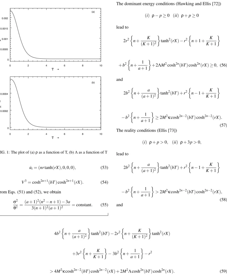
From Eq. (47), we note thatρ(t)is a decreasing function of time andρ>0 for all times. Fig. 1(a) shows this behaviour of energy density.
In spite of homogeneity at large scale our universe is inho-mogeneous at small scales, so physical quantities being po-sition dependent are more natural in our observable universe if we do not go to super high scale. This result shows this kind of physical importance. In recent time theΛ-term has in-terested theoreticians and observers for various reasons. The nontrivial role of the vacuum in the early universe generate a
Λ-term that leads to inflationary phase. Observationally, this term provides an additional parameter to accommodate con-flicting data on the values of the Hubble constant, the decel-eration parameter, the density parameter and the age of the universe (for example, see the references [65, 66]). Assuming thatΛowes its origin to vacuum interactions, as suggested in particular by Sakharov [67], it follows that it would in gen-eral be a function of space and time coordinates, rather than a strict constant. In a homogeneous universeΛwill be at most time dependent [68]. In our case this approach can generateΛ
that varies both with space and time. In considering the nature of local massive objects, however, the space dependence ofΛ
cannot be ignored. For details discussion, the readers are ad-vised to see the references (Narlikar, Pecker and Vigier [69], Ray and Ray [70], Tiwari, Ray and Bhadra [71]).
The behaviour of the universe in this model will be deter-mined by the cosmological term Λ; this term has the same
effect as a uniform mass densityρe f f =−Λ/4πG, which is constant in space and time. A positive value ofΛcorresponds to a negative effective mass density (repulsion). Hence, we expect that in the universe with a positive value ofΛ, the ex-pansion will tend to accelerate; whereas in the universe with negative value ofΛ, the expansion will slow down, stop and reverse. From Eq. (50), we see that the cosmological term
Λis a decreasing function of time and it approaches a small positive value at late time. From Fig. 1(b) we note this be-haviour of cosmological term Λ. Recent cosmological ob-servations (Garnavich et al. [54], Perlmutter et al. [51], Riess et al. [52, 57], Schmidt et al. [56]) suggest the exis-tence of a positive cosmological constantΛ with the magni-tudeΛ(G/c3)≈10−123. These observations on magnitude and red-shift of type Ia supernova suggest that our universe may be an accelerating one with induced cosmological density through the cosmologicalΛ-term. Thus, our model is consis-tent with the results of recent observations.
The kinematical quantities , i.e. the scalar of expansion(θ), shear tensor(σ), the acceleration vector(u˙i)and the proper volume(V3)for the model (44) are given by
θ= b(n+1)tanh(bT)
Mcoshn(bT)coshn(rX), (51)
σ2=b
2tanh2(bT)[(a+1)2(n2−n+1)−3a] 3(a+1)2M2cosh2n(bT)
0 2 4 6 8 10 0
0.0005 0.001 0.0015 0.002
(a)
0 2 4 6 8 10
0 0.0002 0.0004
(b)
FIG. 1: The plot of (a)ρas a function of T, (b)Λas a function of T
˙
ui= (nrtanh(rX),0,0,0), (53)
V3=cosh2n+1(bT)cosh2n+1(rX). (54) From Eqs. (51) and (52), we obtain
σ2
θ2 =
(a+1)2(n2−n+1)−3a
3(n+1)2(a+1)2 =constant. (55)
The dominant energy conditions (Hawking and Ellis [72])
(i) ρ−p≥0 (ii) ρ+p≥0 lead to
2r2
n+ K
(K+1)2
tanh2(rX)−r2
n+1+ K
K+1
+b2
n+ 1
a+1
+2ΛM2cosh2n(bT)cosh2n(rX)≥0, (56)
and
2b2
n+ a
(a+1)2
tanh2(bT) +r2
n−1+ K
K+1
−b2
n+ 1
a+1
≥2M2κcosh2n−2(bT)cosh2n−2(rX).
(57) The reality conditions (Ellis [73])
(i) ρ+p>0, (ii) ρ+3p>0,
lead to
2b2
n+ a
(a+1)2
tanh2(bT) +r2
n−1+ K
K+1
−b2
n+ 1
a+1
>2M2κcosh2n−2(bT)cosh2n−2(rX),
(58) and
4b2
n+ a
(a+1)2
tanh2(bT)−2r2
n+ K
(K+1)2
tanh2(rX)
+3r2
n+ K
K+1
−3b2
n+ 1
a+1
−r2
>4M2κcosh2n−2(bT)cosh2n−2(rX) +2M2Λcosh2n(bT)cosh2n(rX). (59)
In general, the model represents an expanding, shearing and non-rotating universe. Since σθ =constant, hence the model does not approach isotropy. In presence of uniform magnetic
V. SOLUTIONS OF THE FIELD EQUATIONS IN ABSENCE OF MAGNETIC FIELD
In absence of the magnetic field i.e. H=0, the physical parameters, i.e. the pressure(p), the energy density(ρ), the
string tension density(λ), the particle density(ρp)and the cosmological termΛ(t)for the model (44) are given by
p= 1
M2cosh2n(bT)cosh2n(rX)
b2
n+ a
(a+1)2
tanh2(bT)
−r2
n+ K
(K+1)2
tanh2(rX)−b2
n+ 1 (a+1)
+r2
n+ K
(K+1)
−Λ, (60)
λ= 1
M2cosh2n(bT)cosh2n(rX)
r2
n+ K
(K+1)
−b2
n+1+ 1 (a+1)
−2r2
n+ K
(K+1)2
tanh2(rX) , (61)
ρ= 1
M2cosh2n(bT)cosh2n(rX)
b2
n+ a
(a+1)2
tanh2(bT)
+r2
n+ K
(K+1)2
tanh2(rX)−r2 +Λ, (62)
ρp=ρ−λ=
1
M2cosh2n(bT)cosh2n(rX)
b2
n+ a
(a+1)2
tanh2(bT)
+3r2
n+ K
(K+1)2
tanh2(rX) +b2
n−1+ 1 (a+1)
−r2
n+1+ K (K+1)
+Λ. (63)
By using the equation of state (49) in Eqs. (60) and (62), we obtain
Λ= 1
(1−γ)M2cosh2n(bT)cosh2n(rX)
(1−γ)b2
n+ a
(a+1)2
tanh2(bT)
−(1+γ)r2
n+ K
(K+1)2
tanh2(rX)−b2
n+ 1 (a+1)
+r2
n+ K
(K+1)
−γr . (64)
We observe that in absence of the magnetic field, the ex-pressions for Kinematical quantities for the model (44) are
0 2 4 6 8 10 0
0.001 0.002
0.003 (a)
0 2 4 6 8 10
0 0.0002 0.0004 0.0006 0.0008 0.001
(b)
FIG. 2: The plot of (a)ρas a function of T, (b)Λas a function of T
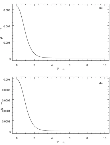
From Eq. (62), we note thatρ(t)is a decreasing function of time andρ>0 for all times. Fig. 2(a) shows this behaviour of
ρ(t). From Eq. (64), we see that the cosmological termΛis a decreasing function of time and it approaches a small positive value as time increases more and more which matches with recent observations. From Fig. 2(b) we note this behaviour of cosmological termΛ. In absence of uniform magnetic field if we setp=0 andΛ=0, our solution represents the solution obtained by Pradhan et al. [61]).
VI. CONCLUDING REMARKS
We have obtained a new cylindrically symmetric inhomo-geneous cosmological model of uniform electromagnetic per-fect fluid as the source of matter where the cosmological con-stant is varying with time. Generally the model represents an expanding, shearing and non-rotating universe in which the flow vector is geodetic. The model does not approach isotropy.
In presence and absence of magnetic field, the cosmolog-ical terms in the models are decreasing function of time and
approach a small value at late time. The values of cosmo-logical “constant” for the models are found to be small and positive, which is supported by the results from supernovae observations recently obtained by the High-Z Supernovae Ia Team and Supernova Cosmological Project (Garnavich et al. [54], Perlmutter et al. [51], Riess et al. [52, 57], Schmidt et al. [56]).
If we setp=0 andΛ=0, our solution represents the so-lution obtained by Pradhan, Rai and Singh [62]. Again we observe that whenp=0,Λ=0, andκ=0, our solution rep-resents the model (case (i)) obtained by Pradhan et al. [61]. Thus our solutions generalize the rsults obtained in [61] and [62].
Acknowledgements
[1] Ya. B. Zel’dovich, I. Yu. Kobzarev, and L. B. Okun, Zh. Eksp. Teor. Fiz.67, 3 (1975); Sov. Phys.-JETP40, 1 (1975). [2] T. W. B. Kibble, J. Phys. A: Math. Gen.9, 1387 (1976). [3] T. W. B. Kibble, Phys. Rep.67, 183 (1980).
[4] A. E. Everett, Phys. Rev.24, 858 (1981). [5] A. Vilenkin, Phys. Rev. D24, 2082 (1981).
[6] Ya. B. Zel’dovich, Mon. Not. R. Astron. Soc.192, 663 (1980). [7] P. S. Letelier, Phys. Rev. D20, 1249 (1979).
[8] P. S. Letelier, Phys. Rev. D28, 2414 (1983). [9] J. Stachel, Phys. Rev. D21, 2171 (1980).
[10] Ya. B. Zel’dovich, A. A. Ruzmainkin, and D. D. Sokoloff, Magnetic field in Astrophysics, Gordon and Breach, New Yark, (1983).
[11] E. R. Harrison, Phys. Rev. Lett.30, 188 (1973).
[12] H. P. Robertson and A. G. Walker, Proc. London Math. Soc.42, 90 (1936).
[13] C. W. Misner, K. S. Thorne, and J. A. Wheeler,Gravitation, W. H. Freeman, New York, (1973).
[14] E. Asseo and H. Sol, Phys. Rep.6, 148 (1987). [15] R. Pudritz and J. Silk, Astrophys. J.342, 650 (1989).
[16] K. T. Kim, P. G. Tribble, and P. P. Kronberg, Astrophys. J.379, 80 (1991).
[17] R. Perley and G. Taylor, Astrophys. J.101, 1623 (1991). [18] P. P. Kronberg, J. J. Perry, and E. L. Zukowski, Astrophys. J.
387, 528 (1991).
[19] A. M. Wolfe, K. Lanzetta, and A. L. Oren Astrophys. J.388, 17 (1992).
[20] R. Kulsrud, R. Cen, J. P. Ostriker, and D. Ryu Astrophys. J.
380, 481 (1997).
[21] J. D. Barrow, Phys. Rev. D55, 7451 (1997).
[22] M. A. Melvin, Ann. New York Acad. Sci.262, 253 (1975). [23] A. Banerjee, A. K. Sanyal, and S. Chakraborty, Pramana-J.
Phys.34, 1 (1990).
[24] S. Chakraborty, Ind. J. Pure Appl. Phys.29, 31 (1980). [25] R. Tikekar and L. K. Patel, Gen. Rel. Grav.24, 397 (1992). [26] R. Tikekar and L. K. Patel, Pramana-J. Phys.42, 483 (1994). [27] L. K. Patel and S. D. Maharaj, Pramana-J. Phys.47, 1 (1996). [28] S. Ram and T. K. Singh, Gen. Rel. Grav.27, 1207 (1995). [29] J. Carminati and C. B. G. McIntosh, J. Phys. A: Math. Gen.13,
953 (1980).
[30] G. P. Singh and T. Singh, Gen. Rel. Grav.31, 371 (1999). [31] G. P. Singh, Nuovo Cim. B110, 1463 (1995); Pramana-J. Phys.
45, 189 (1995).
[32] J. E. Lidsey, D. Wands, and E. J. Copeland, Phys. Rep.337, 343 (2000).
[33] R. Bali and R. D. Upadhaya, Astrophys. Space Sci. 283, 97 (2003).
[34] R. Bali and Anjali, Astrophys. Space Sci.302, 201 (2006). [35] R. Bali, U. K. Pareek, and A. Pradhan, Chin. Phys. Lett.24,
2455 (2007).
[36] R. Bali and A. Tyagi, Gen. Rel. Grav.21, 797 (1989).
[37] A. Pradhan, I. Chakrabarty, and N. N. Saste, Int. J. Mod. Phys. D10, 741 (2001).
[38] A. Pradhan, P. K. Singh, and K. Jotania, Czech. J. Phys.56, 641 (2006).
[39] J. D. Barrow and K. E. Kunze, Phys. Rev. D56, 741 (1997). [40] J. D. Barrow and K. E. Kunze, Phys. Rev. D57, 2255 (1998). [41] L. M. Krauss and M. S. Turner, Gen. Rel. Grav. 27, 1137
(1995).
[42] Ken Croswell, New ScientistApril, 18 (1994).
[43] B. Ratra and P. J. E. Peebles, Phys. Rev.D 37, 3406 (1988).
[44] A. D. Dolgov, in The Very Early Universe, eds. G. W. Gib-bons, S. W. Hawking, and S. T. C. Siklos, Cambridge University Press, Cambridge, (1983);
A. D. Dolgov, M. V. Sazhin, and Ya. B. Zeldovich,Basics of Modern Cosmology, Editions Frontiers, (1990);
A. D. Dolgov, Phys. Rev.D 55, 5881 (1997).
[45] V. Sahni and A. Starobinsky, Int. J. Mod. Phys.D 9, 373 (2000). [46] S. Weinberg,Gravitation and Cosmology, Wiley, New Yark,
(1971).
[47] S. M. Carroll, W. H. Press, and E. L. Turner, Ann. Rev. Astron. Astrophys.30, 499 (1992).
[48] P. J. E. Peebles, Rev. Mod. Phys.75, 559 (2003). [49] T. Padmanabhan, Phys. Rep.380, 235 (2003).
T. Padmanabhan,Dark Energy and Gravity, gr-qc/0705.2533 (2007).
[50] A. Pradhan and H. R. Pandey, Int. J. Mod. Phys.D 12, 941 (2003).
A. Pradhan and O. P. Pandey, Int. J. Mod. Phys.D 12, 1299 (2003).
A. Pradhan, S. K. Srivastav, and K. R. Jotania, Czech. J. Phys.
54, 255 (2004).
A. Pradhan and S. Singh, Int. J. Mod. Phys.D 13, 503 (2004). A. Pradhan, A. K. Yadav, and L. Yadav, Czech. J. Phys.55, 503 (2005).
A. Pradhan and P. Pandey, Czech. J. Phys.55, 749 (2005). A. Pradhan and P. Pandey, Astrophys. J.301, 221 (2006). A. Pradhan, G. P. Singh, and S. Kotambkar, Fizika B,15, 57 (2006).
A. Pradhan, A. K. Singh, and S. Otarod, Roman. J. Phys.52, 415 (2007).
C. P. Singh, S. Kumar, and A. Pradhan, Class. Quantum Grav.
24, 455 (2007).
[51] S. Perlmutter et al., Astrophys. J.483, 565 (1997); Nature391, 51 (1998); Astrophys. J.517, 565 (1999).
[52] A. G. Riess et al., Astron. J.116, 1009 (1998). [53] A. Vilenkin, Phys. Rep.121, 265 (1985).
[54] P. M. Garnavich et al., Astrophys. J.493, L53 (1998a); Astro-phys. J.509, 74 (1998b).
[55] M. Carmeli and T. Kuzmenko, Int. J. Theor. Phys. 41, 131 (2002);
S. Behar and M. Carmeli, Int. J. Theor. Phys.39, 1375 (2002). [56] B. P. Schmidt et al., Astrophys. J.507, 46 (1998).
[57] A. G. Riess et al., Astrophys. J.607, 665 (2004). [58] R. K. Knop et al., Astrophys. J.598, 102 (2003).
[59] H. Baysal, I. Yavuz, I. Tarhan, U. Camci, and I. Yilmaz, Turk. J. Phys.25, 283 (2001).
[60] C. B. Kiline and I. Yavuz, Astrophys. Space Sci. 238, 239 (1996).
[61] A. Pradhan, M. K. Mishra, and A. K. Yadav, gr-qc/0705.1765 (2007).
[62] A. Pradhan, A. Rai, and S. K. Singh, Astrophys. Space Sci.312, 261 (2007).
[63] A. Lichnerowica,Relativistic Hydrodynamics and Magnetohy-drodynamics, W. A. Benjamin Inc., New York, p. 93 (1967). [64] J. L. Synge, Relativity: The General Theory, North-Holland
Publ. Co., Amsterdam, p. 356 (1960).
[65] J. Gunn and B. M. Tinsley, Nature,257, 454 (1975).
[66] E. J. Wampler and W. L. Burke, inNew Ideas in Astronomy (Eds. F. Bertola, J. W. sulentic, and B. F. Madore), Cambridge University Press, p. 317 (1988).
(translation, Soviet Phys. Doklady,12, 1040 (1968)). [68] P. J. E. Peebles and B. Ratra, Astrophys. J.325, L17 (1988). [69] J. V. Narlikar, J. -C. Pecker, and J. -P. Vigier, J. Astrophys. Astr.
12, 7 (1991).
[70] S. Ray and D. Ray, Astrophys. Space Sci.203, 211 (1993). [71] R. N. Tiwari, S. Ray, and S. Bhadra, Indian Pure Appl. Math.
31, 1017 (2000).
[72] S. W. Hawking and G, F, R. Ellis,The Large-scale Structure of Space Time, Cambridge University Press, Cambridge, p. 94, (1973).