A Numerical Study of the Kullback-Leibler Distance
in Functional Magnetic Resonance Imaging
Brenno Caetano Troca Cabella, M´arcio J´unior Sturzbecher, Walfred Tedeschi, Oswaldo Baffa Filho, Dr´aulio Barros de Ara´ujo, and Ubiraci Pereira da Costa Neves
Departamento de F´ısica e Matem´atica,
Faculdade de Filosofia Ciˆencias e Letras de Ribeir˜ao Preto, Universidade de S˜ao Paulo,
Av. Bandeirantes, 3900, 14.040-901, Ribeir˜ao Preto, SP, Brazil
Received on 01 December, 2007
The Kullback-Leibler distance (or relative entropy) is applied in the analysis of functional magnetic resonance (fMRI) data series. Our study is designed for event-related (ER) experiments, where a brief stimulus is presented and a long period of rest is followed. In particular, this relative entropy is used as a measure of the “distance” between the probability distributionsp1andp2of the signal levels related to stimulus and non-stimulus. In order
to avoid undesirable divergences of the Kullback-Leibler distance, a small positive parameterδis introduced in the definition of the probability functions in such a way that it doesnotbias the comparison between both distributions. Numerical simulations are performed so as to determine the probability densities of the mean Kullback-Leibler distanceD(throughout theNepochs of the whole experiment). For small values ofN(N<30), such probability densities f(D)are found to be fitted very well by Gamma distributions (χ2<0.0009). The
sensitivity and specificity of the method are evaluated by construction of the receiver operating characteristic (ROC) curves for some values of signal-to-noise ratio (SNR). The functional maps corresponding to real data series from an asymptomatic volunteer submitted to an ER motor stimulus is obtained by using the proposed technique. The maps present activation in primary and secondary motor brain areas. Both simulated and real data analyses indicate that the relative entropy can be useful for fMRI analysis in the information measure scenario.
Keywords: fMRI Analysis; Kullback-Leibler Distance; Hypothesis Testing
I. INTRODUCTION
The functional magnetic resonance imaging (fMRI) is one of the main techniques for mapping human brain activity in a noninvasive way [1]. This technique allows to assess cogni-tive functions with high spatial and temporal resolution imag-ing. Neural activity due to stimulation causes an increase of the blood flow and oxygenation in the local vasculature. The blood oxygenation level dependent (BOLD) contrast of the image is induced by changes in relative concentrations of oxy and deoxy-hemoglobin [2–4]. The BOLD signal is the re-sponse of the application of an experimental protocol (known as paradigm) which is composed of periodic changes between stimulus and non-stimulus of different brain areas. The result of such an experiment is a time series corresponding to the sig-nal for each voxel. In the processing of fMRI time series, sev-eral methods that separate the physiologically induced signals (corresponding to active voxels) from noise (non-active vox-els) have been employed. Deterministic methods quantify the similarity between the time series of each voxel with a hemo-dynamic response function (HRF) model. On the other hand, statistical methods can infer how significative is the difference between the signals corresponding to periods of stimulation and non-stimulation but do not needa prioriknowledge of the form of the HRF. In the late years, methods based on informa-tion measures, such as the Shannon and Tsallis entropies and the generalized mutual information, have been employed as alternatives for the conventional analysis of fMRI data [5–9].
These informational methods also present the advantage of not requiring a HRF model.
In this context, we now propose to use the Kullback-Leibler distance (or relative entropy) as an information measure to analyse fMRI data series. Our study is designed for event-related (ER) paradigms, where stimulation is presented in a short period of time and followed by a long period of rest. Like other informational methods, the proposed technique only considers the general structure of the signal and needs no HRF model. Indeed the relative entropy is able to quantify the difference between the probability distributionsp1andp2
II. RELATIVE ENTROPY
In information theory, the relative entropy is a measure of the “distance” between the probability functionsp1andp2of
two discrete random variablesX1andX2, respectively. This
information measure is also known as the Kullback-Leibler distance (D) and defined as [10]
D= L
∑
j=1p1jlog2
p1j p2j
, (1)
wherepi jis the probability thatXiassumes thej-th value from its set ofLelements. The logarithm is taken to base 2 so as the entropy is measured in bits.
Relative entropy is not symmetric and is always non-negative. It is zero if and only if p1 = p2. It
should also be noted that lim
p1j→0
p2j=0 p1jlog2
p
1j p2j
=0 whereas
lim
p2j→0 p1j=0
p1jlog2
p
1j p2j
=∞.
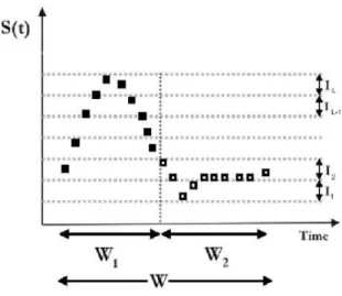
The relative entropy of the time courses(t)of a signal (from real or even simulated data) is proposed to be calculated as follows. Consider one single event-related trial (also named epoch). During that epoch the time courses(t)of the (sim-ulated) BOLD signal of an active voxel exhibits a peak and then returns to a baseline level (Fig.1). As for the calculation of Shannon entropy in a previous work [7], an entire epoch (windowW) of the experiment is divided into two time inter-vals: half windowsW1(related to the signal increase) andW2
(corresponding mainly to baseline values). The probability distribution of signal levels (p1) corresponding to the BOLD
response in the first time period is clearly expected to differ from that one (p2) corresponding to the baseline signal values
so that the relative entropy within this epoch is calculated as a measure of the “distance” between p1and p2. In this way
we consider the discrete setsS1={s(tk),k=1,2, ...,n1}and
S2={s(tl),l=n1+1,n1+2, ...,n1+n2}of signal amplitudes
measured atn1instants(t1<t2< ... <tn1)within periodW1
andn2instants(tn1+1<tn1+2< ... <tn1+n2)within periodW2,
respectively. In order to compute the probability functionsp1
andp2, the accessible states of the system are then defined in
terms of subdivisions of the interval of variation of the sig-nal amplitude [5]. Consider the whole setS=S1∪S2 and
lets0=min[S]andsL=max[S]be the inferior and superior limits ofS, respectively. An equipartition ofSis defined by the amplitude values s0,s1=s0+∆s,s2=s0+2∆s, ...,sL= s0+L∆swhereLis the number of subdivisions (levels) and
∆s= (sL−s0)/L. It is assumed that each subdivision
cor-responds to a possible state of the system. Each integer j from the label set ζ={1,2, ...,L} refers to the thej-th dis-joint intervalIjwhich is defined as[sj−1,sj)(for j≤L−1) and[sL−1,sL](for j=L).
As already noted, the relative entropy might diverge in the limitp2j→0 (forp1j=0). From a practical point of view, this undesirable divergence would be susceptible to occur if the probability functionp2were allowed to assume null values. In
order to avoid such divergence, we introduce a small positive parameterδ(0<δ≤1) in the definition of the probabilities of the signal levels,
pi j= ni j+δ ni+Lδ
, (2)
whereni j= Si∩Ij
is the number of points within window Wi(i=1,2) and levelIj (j=1,2, . . . ,L) andni=|Si|is the whole number of points in windowWi. In the above defini-tion, the condition∑Lj=1pi j=1 is clearly satisfied whereas if δ→0+thenpi j→
ni j
ni so that one recovers the usual meaning
thatpi jis the probability of occupation of levelIj(withinWi), i.e., the relative frequency of points onIj. Furthermore, eq. 2 might be interpreted as the relative frequency of points on levelIj (withinWi)given that a fractionary point (of weight δ) is equally placed on each levelIjof both windowsW1and
W2. In this sense, the introduction of parameter δdoes not
bias the comparison between distributionsp1andp2since it
still remains balanced.
FIG. 1: Time course of the BOLD signal in a single activated voxel. The plot illustrates the set of points within the time interval related to signal increase(W1)and the set of points within the second time
interval(W2)corresponding mainly to baseline values. The intervals I1,I2, ...,ILdefine the accessible levels (states) of the signal.
III. SIMULATED DATA ANALYSIS
two gamma functions,
h(t) =t d
a
exp
d−t
b
−ct d′
a′
exp
d′−t
b′
, (3)
whered=abis the time corresponding to the peak andd′= a′b′is the time for the undershoot, witha=6,a′=12,b= b′=0.9 andc=0.35.
Noiseηis sampled from a gaussian distribution with mean zero and a given varianceσ2
n. Otherwise the varianceσ2sof the signalh(t)is evaluated once along time and is the same for all simulations. Time coursess(t)are simulated for different values of SNR (signal-to-noise ratio) which is usually defined as
SNR=10 log
σ2
s σ2
n
(4) and measured in decibels (dB).
Following the same parameters used in the real ER-fMRI experiment (see section IV), each simulated time courses(t) consists ofN=24 epochs. For each epoch,n1=n2=7 signal
amplitudes are simulated within windowsW1andW2. Some
time seriess(t)simulated for different signal-to-noise ratios (-4dB, 0dB, 4dB and 8dB) are plotted in Fig. 2.
FIG. 2: Plot of some time coursess(t) =h(t) +ηsimulated for dif-ferent SNR’s.
To determine the probability functions p1andp2, we have
chosen the parametersL=2 andδ=0.1 for evaluation of eq. 2. As we shall see, that choice forδleads to optimum results. The Kullback-Leibler distance D must be computed within each epoch. The mean Kullback-Leibler distance Dis the sample average of theNdistances computed along the whole time course. We performNexp=106simulations of the whole time series. Results from simulations show that the Kullback-Leibler distanceDexhibits a discrete probability distribution with periodic peaks. On the other hand, the probability den-sity of the mean distance, f(D), is observed to approach a
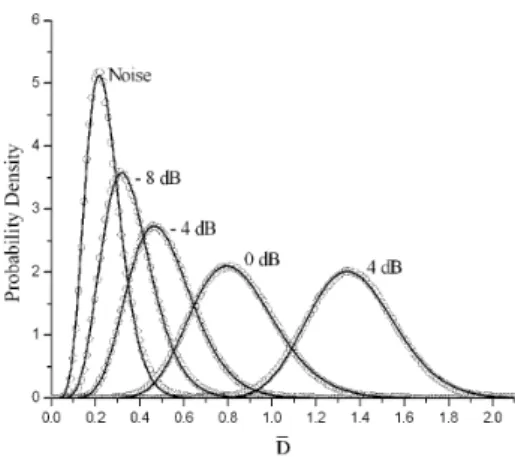
continuous distribution for large values ofN. According to the central limit theorem, f(D)tends to a Gaussian distribu-tion asN→∞. However, for small values ofN(N<30), we have found that the probability densities f(D) can be fitted very well by Gamma distributions,
f(D)≈ D
(α−1)
βαΓ(α)exp
−D
β
, (5)
whereα andβ are parameters of the distribution related to its meanµ=αβand varianceσ2=αβ2. Fig. 3 presents the
probability densities f(D)corresponding to simulations for pure noise (SNR→ −∞) and some finite values of SNR (-8dB, -4dB, 0dB and 4dB); the continuous curves correspond to the Gamma fittings (χ2<0.0009) and overlap the simulated
points very well.
FIG. 3: Probability densitiesf(D)for simulations of pure noise and some finite values of SNR with parametersN=24,n1=n2=7, L=2 andδ=0.1. The continuous curves corresponding to Gamma fittings (χ2<0.0009) overlap the simulated points.
The mean Kullback-Leibler distanceDis elected as the sta-tistic for testing the null hypothesisH0that the time course
s(t) in a particular voxel is pure noise (non-active voxel) against the alternative hypothesisH1thats(t)is composed of
both BOLD signal and noise with a given signal-to-noise ratio (active voxel).
A signal detection scheme can be usually appraised by the construction of the receiver operating characteristic (ROC) curves [14, 15]. In the present analysis, the outcome of the signal detection scheme is the mean distanceD. Such out-come is classified as signal (+) if the observedDbelongs to a given critical region (above some thresholdDc); otherwise it is classified as noise (−). Iff(D|−)and f(D|+)are the prob-ability densities obtained from simulations of pure noise and signal (with a given SNR), respectively, then thesensitivityis defined as the probability of a true positive,
P(+|+) =
∞
Dc
f(D|+)dD, (6)
negative,
P(−|−) = Dc
−∞
f(D|−)dD (7)
(the probability functions are null forD<0). Fig. 4 illustrates the areas under the probability distributions f(D|−)(for noise only) and f(D|+)(for signal with SNR=-4dB) which corre-spond to specificity and sensitivity, respectively. In hypothesis testing, a type I error consists of rejecting the null hypothesis H0when it is true. The significance levelαPT per test is the probability of a type I error, i.e.,αPT=P(+|−) =1−P(−|−) is the probability of a false positive (or 1-specificity).
FIG. 4: Areas corresponding to specificity and sensitivity under probability densitiesf(D|−)(for simulated noise only) and f(D|+) (for simulated signal with SNR=-4dB).
The ROC curve is the plot of sensitivity (probability of a true positive) versus 1-specificity (probability of a false pos-itive), resulting from the variation of the thresholdDc. The ROC curves for several SNR’s are shown in Fig.5.
FIG. 5: ROC curves for different values of SNR.
The performance of the method is evaluated by its ability to detect active brain areas with high sensitivity and speci-ficity. Thus the higher is the concentration of points in the left
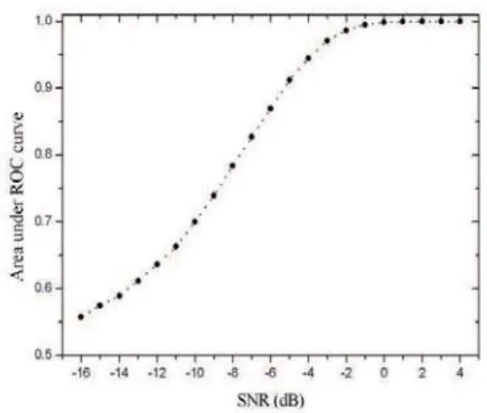
superior corner of the ROC curve graph, the better is the per-formance. Theareabelow the ROC curve is a way to quantify this performance. The discriminate power of the test increases as the ROC area varies from 0.5 (lowest value) to 1 (optimum performance). Our simulations show that the ROC area (and so the discriminate power) grows as SNR is increases accord-ing to Fig. 6. Finally, we may investigate the dependence of the power of the test with the choice of parameterδ. Fig. 7 shows that the ROC area varies smoothly withδfor various SNR’S and thatδ=0.1 seems to be the best choice for all studied cases.
FIG. 6: Area under ROC curve for different values of SNR.
FIG. 7: Area under ROC curve for different values ofδ.
IV. REAL DATA ANALYSIS
re-peated epochs with two states: left- and right-handed finger-tapping with duration of 3-5 seconds and 17-21 seconds of rest. Three axial slices (Fig.8) with 4 mm of width (located on portions of the primary motor cortex) showed 14 temporal points throughout each epoch, three during the activity states and eleven during the period of rest, totalizing 336 images each slice. All images were acquired with echo-planar image (EPI) protocol with repetition time (TR) of 1680 ms, time to echo of 118 ms, flip angle of 90. Each slice was acquired with field of view (FOV) of 210 mm with a matrix 128 x 128 resulting a resolution of 1,64 x 1,64. Preprocessing was car-ried out using the Brain VoyagerTM QX (Brain Innovation Inc., The Netherlands) software. The data analysis included several steps as motion correction, time series image realign-ment by the first slice as reference, spatial smoothing with a FWHM of 4 mm and temporal filtering with a high pass filter of 3 cycle/s.
FIG. 8: Axial Slice.
For each voxel of the image, the mean Kullback-Leibler distance (D) of the corresponding real data series has been computed (with parametersL=2 andδ=0.1). One should remember that this processing requiresnomodel for the HRF. The result of such analysis are the activation maps (overlaid onto corresponding anatomical images) for three axial slices, as shown in Fig. 9. The maps present activation in primary and secondary motor areas due to a motor stimulus. In order to avoid a lot of spurious activated voxels (false positives) in the functional maps, one should consider the ˇSidak` −Bon f erroni correction [16],
αPF=1−(1−αPT)C, (8) whereαPFis the significance level per family of tests, defined as the probability of making at least one type I error for the whole family of tests (i.e., for all voxels); αPT is the usual significance level (per test) andCis the number of tests (vox-els). For a signicance levelαPF=0.05 per family of tests, the threshold for voxel activation isDc=0.9337 so that voxels withD<Dcare decided to be non-active.
V. CONCLUSION
In summary, we have proposed the use of the Kullback-Leibler distance (or relative entropy) as an alternative method
to analyse fMRI data series. The probability distributions of the mean Kullback-Leibler distance (throughout theNepochs of the event related experiment) were determined by numeri-cal simulations. The sensitivity and specificity of the method
FIG. 9: Functional maps of three axial slices obtained by employ-ment of Kullback-Leibler information measure. For a signicance level per familyαPF=0.05, the threshold for voxel activation is
Dc=0.9337 so that voxels withD<Dcare cut off (non-active).
were evaluated by construction of ROC curves for different SNR’s. The functional map corresponding to real data se-ries from an asymptomatic volunteer submitted to an ER mo-tor stimulus was obtained by using the proposed technique. Our results from both simulated and real data indicate that the technique can be a very good option for fMRI analysis. As a further study, the use of thegeneralized Kullback-Leibler distance in fMRI analysis might be considered.
Acknowledgments
The authors acknowledge the Brazilian agencies CNPq and CAPES for financial support.
[1] D. Lebihan, Diffusion and Perfusion Magnetic Resonance Imaging Applications to Functional MRI, Raven Press, New
[2] S. Ogawa, T. Lee, A. Nayak, P. Glynn,Magnetic Resonance in Medicine14, 68 (1990).
[3] S. Ogawa, T. Lee, A. Kay, D. Tank,Proceedings of the National Academy of Sciences USA, 986887(1990).
[4] P. van Zijl, S. Eleff, J. Ulatowski, J. Oja, A. Ulug, R. Traystman, R. Kauppinen, Nature Medicine4, 159 (1998).
[5] A. Capurro, L. Diambra, D. Lorenzo, O. Macadar, M. T. Martin, C. Mostaccio, A. Plastino, J. P´erez, E. Rofman, M. E. Torres, J. Velluti,Physica A265, 235 (1999).
[6] T. Yamano,Phys. Rev. A63, 046-105 (2001).
[7] D. B. de Araujo, W. Tedeschi, A. C. Santos, J. Elias Jr., U. P. C. Neves, O. Baffa,Neuroimage20, 311 (2003).
[8] W. Tedeschi, D. B. de Araujo, H.-P. M ¨uller, , A. C. Santos, U. P. C. Neves, S. N. Ern`e, O. Baffa,Physica A344, 705-711 (2004). [9] W. Tedeschi, H.-P. M¨uller, D. B. de Araujo, A. C. Santos, U. P.
C. Neves, S. N. Ern`e, O. Baffa,Physica A352, 629-644 (2005). [10] T. M. Cover, J. A. Thomas,Elements of information theory,
John Wiley & Sons, New York, (1991).
[11] F. M. Miezin, L. Maccotta, J. M. Ollinger, S. E. Petersen and R. L. Buckner,NeuroImage11, 735 (2000).
[12] D. Malonek, A. Grinvald,Science272, 551 (1996).
[13] K. J. Friston, P. Fletcher, O. Josephs, A. Holmes, M. D. Rugg, R. Turner,NeuroImage7, 30 (1998).
[14] J. Hanley, B. McNeil,Radiology148, 839 (1983).
[15] D. Goodenough, K. Rossmann, L. Lusted,Radiology110, 89 (1974).