Evaluation of GEOS-5 sulfur dioxide simulations during the Frostburg, MD 2010 field campaign

(1)

ACPD

13, 21765–21800, 2013

Evaluation of GEOS-5 SO2simulations

V. Buchard et al.

Title Page

Abstract Introduction

Conclusions References

Tables Figures

◭ ◮

Back Close

Full Screen / Esc

Printer-friendly Version

Interactive Discussion

Discussion

P

a

per

|

D

iscussion

P

a

per

|

Discussion

P

a

per

|

Discuss

ion

P

a

per

|

Atmos. Chem. Phys. Discuss., 13, 21765–21800, 2013 www.atmos-chem-phys-discuss.net/13/21765/2013/ doi:10.5194/acpd-13-21765-2013

Atmospheric Chemistry and Physics

Open Access

Discussions

Geoscientiic Geoscientiic

This discussion paper is/has been under review for the journal Atmospheric Chemistry and Physics (ACP). Please refer to the corresponding final paper in ACP if available.

Evaluation of GEOS-5 sulfur dioxide

simulations during the Frostburg, MD

2010 field campaign

V. Buchard1,2, A. M. da Silva1, P. Colarco3, N. Krotkov3, R. R. Dickerson4,5, J. W. Stehr4, G. Mount6, E. Spinei6, H. L. Arkinson4, and H. He4

1

Global Modeling and Assimilation Office, NASA Goddard Space Flight Center, Greenbelt, MD, USA

2

Universities Space Research Association, GESTAR, Columbia, MD, USA

3

Atmospheric Chemistry and Dynamics Lab, NASA Goddard Space Flight Center, Greenbelt, MD, USA

4

Department of Atmospheric and Oceanic Science, University of Maryland, College Park, MD, USA

5

Department of Chemistry, University of Maryland, College Park, MD, USA

6

Laboratory for Atmospheric Research, Washington State University, Pullman, WA, USA

Received: 28 June 2013 – Accepted: 7 August 2013 – Published: 22 August 2013

Correspondence to: V. Buchard (virginie.j.buchard-marchant@nasa.gov)

(2)

ACPD

13, 21765–21800, 2013

V. Buchard et al.

Title Page

Tables Figures

◭ ◮

Back Close

Full Screen / Esc

Discussion

P

a

per

|

D

iscussion

P

a

per

|

Discussion

P

a

per

|

Discuss

ion

P

a

per

|

Abstract

Sulfur dioxide (SO2) is a major atmospheric pollutant with a strong anthropogenic

com-ponent mostly produced by the combustion of fossil fuel and other industrial activities. As a precursor of sulfate aerosols that a_ffect climate, air quality, and human health, this gas needs to be monitored on a global scale. Global climate and chemistry

mod-5

els including aerosol processes along with their radiative effects are important tools for climate and air quality research. Validation of these models against in-situ and satellite measurements is essential to ascertain the credibility of these models and to guide model improvements. In this study the Goddard Chemistry, Aerosol, Radiation, and Transport (GOCART) module running on-line inside the Goddard Earth Observing

10

System version 5 (GEOS-5) model is used to simulate aerosol and SO2

concentra-tions. Data taken in November 2010 over Frostburg, Maryland during an SO2 field

campaign involving ground instrumentation and aircraft are used to evaluate GEOS-5 simulated SO2concentrations. Preliminary data analysis indicated the model

overes-timated surface SO2 concentration, which motivated the examination of mixing pro-15

cesses in the model and the specification of SO₂ anthropogenic emission rates. As a result of this analysis, a revision of anthropogenic emission inventories in GEOS-5 was implemented, and the vertical placement of SO2 sources was updated. Results

show that these revisions improve the model agreement with observations locally and in regions outside the area of this field campaign. In particular, we use the

ground-20

based measurements collected by the United States Environmental Protection Agency (US EPA) for the year 2010 to evaluate the revised model simulations over North Amer-ica.

1 Introduction

Sulfur dioxide (SO₂) is a trace gas which poses significant health threats near the

25

(3)

ACPD

13, 21765–21800, 2013

V. Buchard et al.

Title Page

Tables Figures

◭ ◮

Back Close

Full Screen / Esc

Discussion

P

a

per

|

D

iscussion

P

a

per

|

Discussion

P

a

per

|

Discuss

ion

P

a

per

|

on the ecosystem acidification (Schwartz, 1989). With a mean lifetime of few days in the troposphere (Lee et al., 2011; He et al., 2012), emitted SO2 is quickly oxidized to

form sulfate aerosols. The resulting aerosols exert influences on the atmospheric ra-diative balance and cloud microphysics (e.g., McFiggans et al., 2006). SO₂ is emitted into the atmosphere mainly from anthropogenic sources such as fossil fuel

combus-5

tion and industrial facilities. In the US these emissions represent more than 90 % of SO₂ released into the air (US EPA, 2011). Since the implementation of national en-vironmental regulations (e.g. 1990 Clean Air Act Amendments in the United States), a significant decrease of these emissions has been observed over the past 30 yr. To keep track of SO₂emissions, this gas is monitored throughout the country by a system

10

of continuously sampling ground-based instruments, and also by episodic intensive field campaigns. These campaigns are particularly valuable because the instruments deployed on the ground and from aircraft give not only the opportunity to validate and improve the ability of space-based instruments to monitor air pollutants, but also pro-vide the opportunity to evaluate chemical transport models that simulate the SO2and 15

sulfate lifecycle (Chin et al., 2000b; Easter et al., 2004; Liu et al., 2005; Goto et al., 2011). Generally, the studies above found that modeled SO₂concentrations at the sur-face were overestimated over Europe and North America, which could be attributed to too high SO2 emission rates or deficiencies in SO2 losses due to oxidation. Also,

uncertainties in the model surface fields may be di_fferent from the total column, and

20

must be evaluated separately. For example, in the GEOS-5 global model it is possible to constrain the total column aerosol loading through assimilation of aerosol optical depth (AOD) from satellite observations. Assimilation of AOD, however, does not cor-rect errors in either aerosol vertical placement or composition, so it remains important to evaluate these aspects of the model. Here we focus particularly on the surface SO2 25

and sulfate concentrations. The purpose of this paper is to take advantage of the data measured during the Frostburg field campaign held in Maryland during November 2010 to evaluate the SO2simulated with the GEOS-5/GOCART model. We first describe in

(4)

ACPD

13, 21765–21800, 2013

V. Buchard et al.

Title Page

Tables Figures

◭ ◮

Back Close

Full Screen / Esc

Discussion

P

a

per

|

D

iscussion

P

a

per

|

Discussion

P

a

per

|

Discuss

ion

P

a

per

|

chemical processes considered within the model. In Sect. 3 we start by validating the modeled SO2at the surface over the continental US using the data collected by EPA. In

Sect. 4 we evaluate the GEOS-5 simulated SO2 with measurement data taken during

the campaign. Section 5 reports the conclusions.

2 Representation of Aerosols in the GEOS-5 Earth Modeling System

5

The Goddard Earth Observing System version 5 (GEOS-5) model, the latest version from the NASA Global Modeling and Assimilation Office (GMAO), is a weather and climate capable model described by Rienecker et al. (2008). The GEOS-5 system in-cludes atmospheric circulation and composition, oceanic and land components. By including an aerosol transport module based on the Goddard Chemistry Aerosol

Radi-10

ation and Transport (GOCART) model (Chin et al., 2002), GEOS-5 provides the capa-bility of studying atmospheric composition and aerosol–chemistry–climate interaction (Colarco et al., 2010). In addition to providing reanalyses of traditional meteorological parameters (winds, pressure and temperature fields, Rienecker et al., 2008), the inclu-sion of aerosols provides the background information for GEOS-5 to produce

reanaly-15

ses of aerosol fields using retrieved AOD from the space-based instrument Moderate Resolution Imaging Spectroradiometer (MODIS). The GEOS-5 near-real time system runs at a nominal 25 km horizontal resolution with 72 vertical levels between the surface and about 80 km. For this study, the model was run at various horizontal resolutions, 0.25◦

×0.315◦ with sensitivity experiments also carried out at 0.5◦×0.625◦ latitude by 20

longitude.

GEOS-5 can be run in climate simulation, data assimilation, or replay modes. In the data assimilation mode, a meteorological analysis is performed every six hours to constrain the meteorological state of the model. In the replay mode, a previous analysis, generated with the same version of model, is used to adjust the model’s

25

(5)

ACPD

13, 21765–21800, 2013

V. Buchard et al.

Title Page

Tables Figures

◭ ◮

Back Close

Full Screen / Esc

Discussion

P

a

per

|

D

iscussion

P

a

per

|

Discussion

P

a

per

|

Discuss

ion

P

a

per

|

thermodynamical state at every time step between analysis updates. For this study GEOS-5 is run in replay-mode using the GMAO atmospheric analyses from the Modern Era Retrospective analysis for Research and Applications (MERRA) (Rienecker et al., 2011) available every six hours.

The GOCART module simulates five aerosol types: dust, sea salt, black carbon,

5

organic carbon and sulfate aerosol. The sulfur chemistry processes considered are based on Chin et al. (2000a). Sulfate aerosol is mostly formed from the oxidation of SO2. All simulations include emissions of dimethysulfide (DMS), SO2and sulfate and

we use prescribed oxidant fields (hydroxyl radical (OH), nitrate radical (NO₃) and hydro-gen peroxide (H2O2)) from a monthly varying climatology produced from simulations 10

in the NASA Global Modeling Initiative (GMI) model (Duncan et al., 2007; Strahan and Douglas, 2004). A small amount of SO₂ is produced by the oxidation of DMS, which is emitted naturally from marine phytoplankton. We use a monthly varying climatology of oceanic DMS concentrations (Kettle et al., 1999), with emissions calculated using the surface wind-speed dependent (Liss and Merlivat, 1986) parameterizations of

air-15

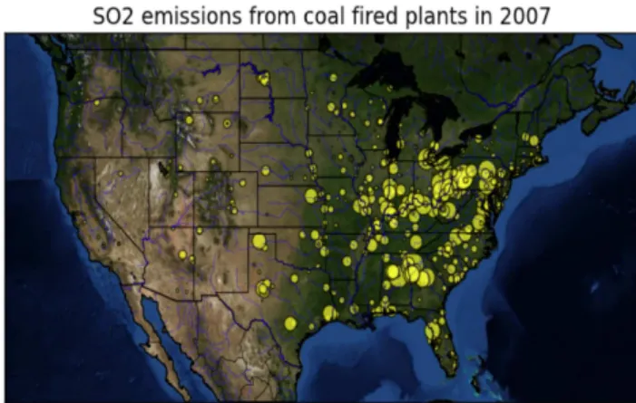
ocean exchange processes. The main source of SO2 is anthropogenic, mainly from

fossil fuel combustion from power plants and industrial activities (US EPA, 2011). Figure 1 maps the emissions of SO₂released from coal fired power plants (in tons) over the US in 2007. In this study, two different data sets of anthropogenic emissions and two assumptions about the injection height are considered in our simulations to

20

assess the e_ffect of the emissions on SO₂ surface concentration. At the time of the campaign, the annual anthropogenic emissions of SO2 were taken from Streets et al.

(2009). In the GEOS-5 control simulation (replay-mode), this emission was injected into the lowest model level. All simulated results using this configuration are hereafter called the “Control Run” or CR.

25

Recently, a new Emission Database for Global Atmospheric Research (EDGAR) ver-sion v4.1 dataset (European Commisver-sion, 2010) became available at 0.5◦ _horizontal

(6)

non-ACPD

13, 21765–21800, 2013

V. Buchard et al.

Title Page

Tables Figures

◭ ◮

Back Close

Full Screen / Esc

Discussion

P

a

per

|

D

iscussion

P

a

per

|

Discussion

P

a

per

|

Discuss

ion

P

a

per

|

energy emissions (from transportation, manufacturing industries, residential) into the lowest GEOS-5 layer and the energy emissions from power plants at higher levels between 100 and 500 m (between the 2nd and 4th model layers). The results (using a replay simulation) are herein referred to as the “Revised Run” or RR.

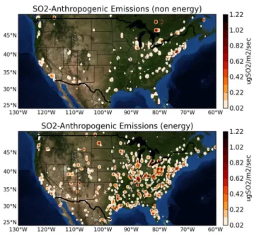
Figure 2 shows a comparison of the SO2 anthropogenic emissions by source cate-5

gory: energy-source sector and non-energy-source sector, based on the EDGAR 2005 database as used in our revised simulation. Most SO₂ emissions are released from power plants, so it is important to consider the emission injection above 100 m due to the stack height and plume rise. We assume these emissions are constant throughout the year. Furthermore, other anthropogenic emissions include aircraft and ship traffic

10

emissions from Mortlock et al. (1998) and Eyring et al. (2005) respectively. We assume 3 % of the SO2anthropogenic emissions are directly emitted as sulfate. All the

simula-tions include also biomass burning emissions of SO2following the Quick Fire Emission

Dataset (QFED) inventory and SO₂ emissions from continuously eruptive volcanoes that are based on data from the Global Volcanism Program database (Siebert et al.,

15

2002) and Total Ozone Mapping Spectrometer (TOMS) and Ozone Monitoring Instru-ment (OMI)’s SO₂ retrievals (Carn et al., 2003; Krotkov et al., 2006) while emissions from explosive volcanoes follow the Aerocom inventories (Dentener et al., 2006). SO2

is removed in the atmosphere by dry and wet deposition and oxidized to sulfate by chemical reaction. The main oxidation pathways for SO₂are the gas phase oxidation

20

by OH and aqueous phase oxidation by H2O2 (Chin et al., 2000a), with the aqueous

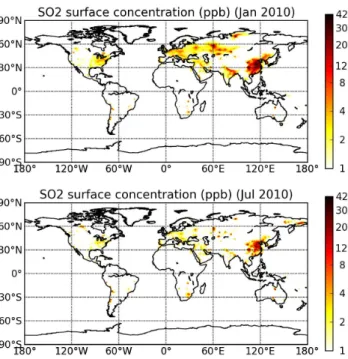
chemistry driven by the GEOS-5 cloud fraction and precipitation, which have been eval-uated separately in (Molod et al., 2012). We save the model tracer fields every three hours during our simulation. Figure 3 shows results of the simulated SO2surface

con-centrations for January and July 2010. The highest SO2concentrations are found over 25

eastern Asia, Europe, and North America, which are major anthropogenic source re-gions. SO2concentrations are higher during the winter; this seasonal variation can be

explained by the seasonal SO2 oxidation rates, which are slower in winter than in the

(7)

re-ACPD

13, 21765–21800, 2013

V. Buchard et al.

Title Page

Tables Figures

◭ ◮

Back Close

Full Screen / Esc

Discussion

P

a

per

|

D

iscussion

P

a

per

|

Discussion

P

a

per

|

Discuss

ion

P

a

per

|

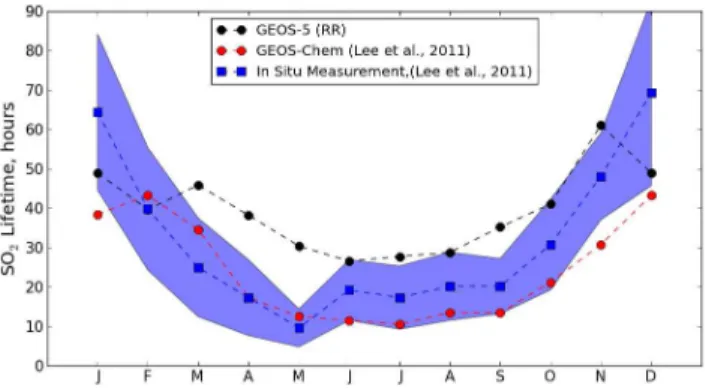
sponsible for this seasonal cycle of SO2 concentrations. Figure 4 shows an evaluation of the GEOS-5 simulation of the SO2 lifetime in black by comparison with the

analy-sis made by Lee et al. (2011) with the GEOS-Chem chemical transport model in red and in-situ measurements-based lifetime in blue. The mean SO₂lifetime from GEOS-5 simulations are calculated over the eastern US (3GEOS-5.2◦_N–44.5◦_{N, 68.4}◦_W–81.6◦_W) 5

and during daytime as Lee et al. (2011) but for the year 2010. The seasonal varia-tion of the SO₂lifetime from GEOS-5 is globally consistent with the seasonal variation found with the GEOS-chem model and the in-situ measurements. While the mean SO2

lifetime from GEOS-chem are generally shorter than the in-situ measurement-based lifetime, the mean SO₂lifetime from GEOS-5 simulations are generally higher than the

10

in-situ measurements, except during the winter. However, the GEOS-5 SO₂ lifetime values are quite close or within the range defined by the uncertainty interval of in-situ measurements. The differences in the transport and in the emissions are among the possible reasons that may explain the discrepancy with the GEOS-Chem model. In addition the oxidant fields in GEOS-5 are not interactive and depend instead on fields

15

from a different model from a different period.

3 Model comparison to EPA surface measurements

In this section we evaluate the modeled surface concentrations of SO2and sulfate over

the US for the control and revised runs for the year 2010. For this study we used data collected by EPA, local and state control agencies which maintain air quality monitoring

20

networks over the US available from the EPA Air Quality System (AQS) (US EPA, 2010).

3.1 Sulfur dioxide

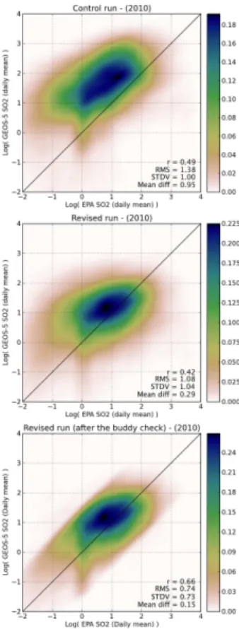
Figure 5 shows the SO₂ daily mean comparisons for the control run (top) and the re-vised run (middle). The “EPA” daily averages of SO2concentration were calculated

us-ing hourly concentrations collected from 102 sites obtained from the EPA AQS. A

(8)

ACPD

13, 21765–21800, 2013

V. Buchard et al.

Title Page

Tables Figures

◭ ◮

Back Close

Full Screen / Esc

Discussion

P

a

per

|

D

iscussion

P

a

per

|

Discussion

P

a

per

|

Discuss

ion

P

a

per

|

nel density estimation (KDE) (Silverman, 1986; Scott, 1992) was applied to approxi-mate the joint probability density function (PDF) of observed and modeled SO2 daily

mean surface concentrations. Since SO2is usually lognormally distributed, the

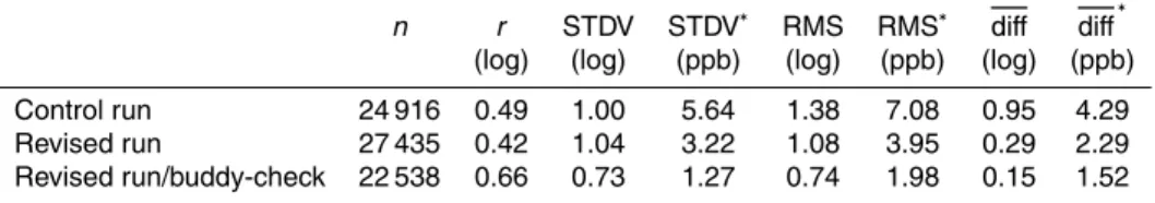
corre-lation coefficientr, the Root Mean Square of the differences (GEOS-5-EPA) (RMS), the standard deviation (STDV) and the mean differences are calculated for

logarithmi-5

cally transformed data (summarized in Table 1 as well as the parameters in the original units calculated using the equations described in Limpert et al., 2001 (Appendix A)). For both plots, the scatter between modeled and observed daily means is significant with correlation coefficients, r ₌0.49 and r ₌0.42 for the control and revised run re-spectively. However, the agreement between the observed and modeled daily mean is

10

better with the revised run, with lower values for the RMS and the mean di_fference. The STDV is almost the same for both the control and revised runs. One of the reasons for this discrepancy might be attributed to the change in absolute magnitude of the SO2

emissions datasets used in the control and revised runs, but we noticed only small dif-ferences between the two datasets. Another plausible explanation is the emission

injec-15

tion height considered in the model. The vertical placement of emissions in the revised run decreases the high bias between observations and simulations at the surface. The remaining bias between observations and revised model SO2simulations may be

ex-plained by the error of representativeness associated with the incompatibility between in-situ measurements and grid-box mean values predicted by the model. As an attempt

20

to filter out the in-situ measurements that are very unrepresentative of the grid-box mean conditions, the bottom plot of Fig. 5 presents the results after a statistical quality control was performed with the adaptive buddy check of Dee et al. (2001). For a given observation, this method consists of looking at nearby model-observations discrepan-cies and discarding those observations that cannot be corroborated by their neighbors.

25

(9)

ACPD

13, 21765–21800, 2013

V. Buchard et al.

Title Page

Tables Figures

◭ ◮

Back Close

Full Screen / Esc

Discussion

P

a

per

|

D

iscussion

P

a

per

|

Discussion

P

a

per

|

Discuss

ion

P

a

per

|

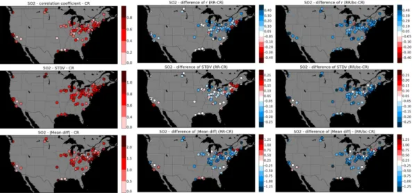
quality control could be the year (2005) of the emission dataset with emissions too high for the year 2010. According to EPA (e.g., http://www.epa.gov/air/airtrends/sulfur.html) the average SO2concentrations have decreased substantially over the years because

of the application of SO₂control measures. Based on 341 US monitor sites, a 60 % de-crease in national average was found between 2000 and 2010. If we look site by site,

5

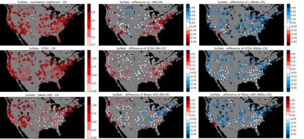
Fig. 6 presents the change in ther (top), the STDV(middle) and the absolute value of the mean difference (bottom) between modeled and observed daily averaged surface SO2 for the control run on the left, the revised run in the middle and after the buddy

check on the right. While the correlation coefficient increased from values lower than 0.4–0.6 for the control run to values greater than 0.6 after the buddy check, we see

10

that the STDV increased over New England and slightly decreased elsewhere for the revised run, the decrease is more significant after the buddy check. Concerning the absolute value of mean difference, we notice a decrease more and more significant between the control, the revised run and after the buddy-check.

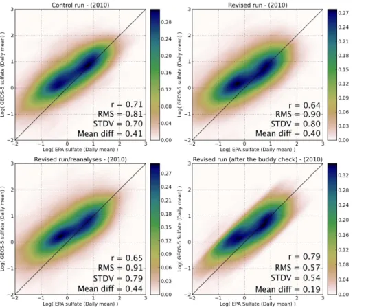
3.2 Sulfate aerosol

15

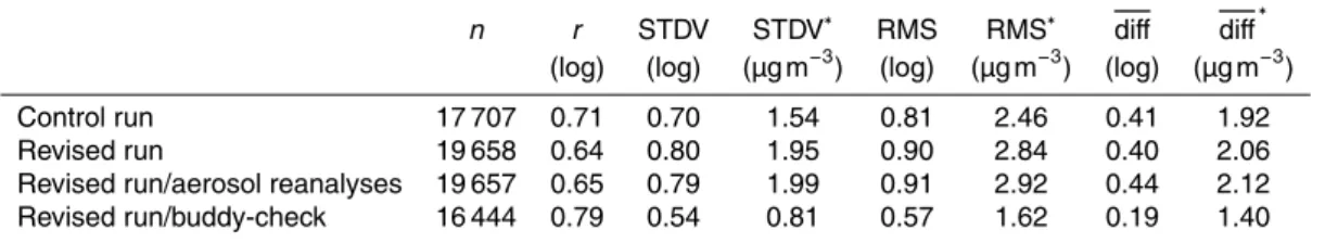
Figure 7 shows comparisons similar to the ones on Fig. 5, but for sulfate. The daily means are directly provided by the EPA AQS and are available every one, three or six days for a total of 250 sites. Figure 7 includes also a comparison with the sulfate sim-ulated with the GEOS-5 aerosol assimilation system, assimilation of MODIS AOD in the revised version of the model has been performed. On average the modeled sulfate

20

concentrations are higher than the observations, regardless of the model or data as-similation system used. The values ofr, the RMS, STDV and the average differences are slightly different for the control, revised simulations and the reanalysis (summarized in Table 2). This suggests that the SO₂ emissions injections as well as the assimila-tion of AOD observaassimila-tions into the model have a low impact on the daily mean sulfate

25

comparisons. Like for the SO2 study, the measurements have been quality controlled

(10)

Cou-ACPD

13, 21765–21800, 2013

V. Buchard et al.

Title Page

Tables Figures

◭ ◮

Back Close

Full Screen / Esc

Discussion

P

a

per

|

D

iscussion

P

a

per

|

Discussion

P

a

per

|

Discuss

ion

P

a

per

|

pled with the longer lifetime of SO₂ in Figs. 4 and 5 and, hence, too slow production of sulfate, our results suggest we may strongly underestimating the losses of sulfate aerosol. When looking site by site (Fig. 8), while the values of r decrease with the re-vised simulations for some sites, the application of the buddy check lead generally to greater and significant correlation coefficient values; the STDV values have not really

5

changed between the control and revised runs but the values tend to decrease after the buddy check. Finally we see also an improvement in the absolute values of the mean differences after the revised and more importantly after the buddy check simulations.

4 Evaluation of SO2 in the model: comparison with measurement data during

the Frostburg campaign in Maryland

10

In Sect. 4 we concentrate our evaluation of the model performance in a smaller region using data collected during an air quality campaign in western Maryland in Novem-ber 2010. The Frostburg campaign was a regional air quality campaign conducted by investigators from Washington State University (WSU), the University of Maryland (UMD) and the NASA Goddard Space Flight Center (GSFC) during two weeks in

15

November 2010. The campaign took place in Western Maryland and provided direct measurements of SO2among other atmospheric constituents. The interest of this

re-gion is based on the abundance of SO2 from the Ohio River Valley, surrounded by

several power plants (Fig. 9). In this section, we make use of several data sets avail-able during this campaign to evaluate the anthropogenic SO2 concentration simulated 20

by GEOS-5.

4.1 Surface analysis: comparisons at Piney Run Station

(11)

ACPD

13, 21765–21800, 2013

V. Buchard et al.

Title Page

Tables Figures

◭ ◮

Back Close

Full Screen / Esc

Discussion

P

a

per

|

D

iscussion

P

a

per

|

Discussion

P

a

per

|

Discuss

ion

P

a

per

|

with the nearest one, Warrior Run, located south of Cumberland. Globally, the model captures the observed month-to-month variability of SO2 with a winter maximum for

both the control run in red and the revised run in black, as stated in Sect. 2, the oxidation rates and the PBL dynamics are responsible for this seasonal variation.

In the control run (the red line in Fig. 10), we see that the model overestimates

5

the observed SO2values by a factor of 4–5. This result is consistent with the general

findings of Sect. 3: the revised vertical placement of SO₂ emissions has a positive impact on the simulated surface values of SO2. This is shown with the revised run

(in black) where the model values are in better agreement with the observations and the overestimation is less than a factor 2. Like seen previously, an explanation of the

10

positive bias remaining might be attributed to the 2005 emissions inventory and the recent decreasing trend of SO2 pollution over the US noted by EPA. In particular in

Piney Run, the concentrations of SO2decreased 50 % between 2006 and 2010.

Figure 11 shows the comparison of the daily mean SO₂ surface concentrations to the measurements at Piney Run during 2010. Again, we see the better agreement

15

between the revised run and the observations.

4.2 Column amount analysis: comparisons to a MF-DOAS instrument

Simulated SO₂column amount is evaluated with measurements from the Multifunction Differential Optical Absorption Spectroscopy (MFDOAS) instrument developed at WSU (Herman et al., 2009; Spinei et al., 2010), deployed on the roof of a building at

Frost-20

burg State University (FSU) for the campaign. This instrument measures the direct sun irradiance and scattered sunlight in spectral UV and visible wavelengths 281–498 nm at 0.83 nm spectral resolution recorded simultaneously with a CCD detector in the spec-trograph focal plane. Analysis of the measured spectra is done using the DOAS tech-nique which is based on the Beer–Lambert law which states that the relationship at

25

(12)

ACPD

13, 21765–21800, 2013

V. Buchard et al.

Title Page

Tables Figures

◭ ◮

Back Close

Full Screen / Esc

Discussion

P

a

per

|

D

iscussion

P

a

per

|

Discussion

P

a

per

|

Discuss

ion

P

a

per

|

with an uncertainty less than 0.03 DU. A description of this instrument as well as the DOAS technique can be found in Spinei et al. (2010). Figure 12 shows the comparison between the column density measured by the MFDOAS and simulated by GEOS-5 during daylight hours from 13:30 UTC until 21:00 UTC on 8 and 9 November. We no-tice that changing from one emission dataset to the other shows not much change on

5

the total column amount between the two runs; it confirms the small changes in the absolute magnitude of the SO₂ emissions between the two datasets. Accounting for the uncertainty on the ground-based instrument, the comparison is rather satisfying with both the control and revised run but we notice that the model does not reproduce the observed diurnal variations. Besides the lack of diurnal variation in the prescribed

10

emissions, an explanation might be the spatial resolution of the model (∼25 km) and

the offset pointing of the MFDOAS instrument when looking at the sun.

4.3 Vertical analysis: comparisons to aircraft measurements

The GEOS-5 simulated vertical distribution of SO2 is compared to aircraft

mea-surements conducted on two di_fferent days during the campaign. The flights were

15

made on the UMD Cessna 402B aircraft, which was equipped with a modified pulse-fluorescence instrument to measure the in situ SO2 concentration (Taubman et al.,

2006). The aircraft flight path on 8 November is shown on Fig. 9. Important regional power plants are marked by yellow circles in Fig. 9, with the size of the circle indicating the magnitude of SO2emissions. 8 November 2010 featured sustained winds as high 20

as 29 km h−1 _{with gusts to 45 km h}−1 _{around the time of the flight. 9 November 2010}

was considerably calmer, with sustained winds under 19 km h−1_{and gusts noted over}

Cumberland around the time of the flight. These information were recorded at the air-port, which is not an official National Weather Service reporting station, but they were also backed up by the informal observations of the airplane’s crew. Both flights lasted

25

about two hours and were characterized by spiraling climbs and descents over Frost-burg (39.65◦_N–78.93◦_{W) and Cumberland, Maryland (39.62}◦_N–78.77◦_{W). Figure 13}

(13)

ACPD

13, 21765–21800, 2013

V. Buchard et al.

Title Page

Tables Figures

◭ ◮

Back Close

Full Screen / Esc

Discussion

P

a

per

|

D

iscussion

P

a

per

|

Discussion

P

a

per

|

Discuss

ion

P

a

per

|

runs sampled along the aircraft flight path, as well as the comparisons of the modeled SO2concentration from the revised run only to the aircraft observations for both days.

The dark black lines in Fig. 13 show the modeled SO2extracted exactly at the aircraft

position, while the blue shading shows the range of the modeled SO₂ concentrations for the surrounded grid boxes (25 km in the horizontal direction and 200 m in the

ver-5

tical direction). If we look at the vertical profiles comparisons between the control and revised runs, we notice small changes between the two runs. On 8 November, GEOS-5 captures most of the major features of the aircraft observations, including the sharp vertical gradient encountered as the aircraft made its vertical profile near Cumberland (at about 60 min of flight time). The turbulent mixing and strong winds during this day

10

explain the air well mixed and coming from a much larger area. On 9 November the model also captures many of the aircraft variations but misses the observed high values between 60–80 min flight time. During this time frame, the aircraft was flying over Cum-berland, near the coal fired power plant Warrior Run. The calmer weather conditions during this day may explain the high values observed locally that could not be

repro-15

duced by the model with a 25 km resolution. Concerning the simulated surface-level SO₂, like seen in more details in Sects. 3.1 and 4.1 we notice a slight overestimation of the SO2surface-level concentration at the beginning and at the end of the flight on

both days.

5 Conclusions

20

The Frostburg campaign that took place in Maryland in November 2010 was a good opportunity to evaluate the SO2simulated by the GEOS-5/GOCART system. By

com-paring the modeled SO₂ against observed data, such as aircraft and ground-based measurements from a ground-based system in Frostburg, we have first diagnosed that the SO2 concentrations was overestimated at the surface and adjusting the vertical 25

(14)

ACPD

13, 21765–21800, 2013

V. Buchard et al.

Title Page

Tables Figures

◭ ◮

Back Close

Full Screen / Esc

Discussion

P

a

per

|

D

iscussion

P

a

per

|

Discussion

P

a

per

|

Discuss

ion

P

a

per

|

The improvement in our treatment of the SO₂anthropogenic emissions was confirmed with the analysis performed over the US using the EPA ground-based measurements.

The comparisons of the vertical profile with aircraft data showed that despite the spa-tial coarse resolution of GEOS-5, most of the major features of the aircraft observations were reproduced by the model on 8 November because the weather was dynamic with

5

turbulent mixing and strong winds. In contrast the analysis on 9 November shows that during quiet days, GEOS-5 will have difficulty of detecting plumes, especially in the vicinity of point source. Concerning the GEOS-5 simulated sulfate, the comparisons with the EPA data show that the changes in the SO2 emissions dataset and vertical

distribution did not affect much the simulation of the sulfate at the surface, the positive

10

bias observed with the control run remains with the revised run. These comparisons suggests that there might have an underestimated loss of sulfate in the model. A full analysis of the chemical processes could not be performed with the available data and there is a possibility that part of this process could also explain part of the bias remain-ing in the SO2and sulfate comparisons.

15

Appendix A

The lognormal distribution

A random variableX is lognormally distributed if Y ₌logX has a normal distribution. The meanX and the standard deviations_X of the normal variable are related to theY ands_Y of the lognormal variable by (Limpert et al., 2001):

20

X₌exp(Y₊s_Y2/2) (A1)

s_X ₌X

q

exp(s_Y2

(15)

ACPD

13, 21765–21800, 2013

V. Buchard et al.

Title Page

Tables Figures

◭ ◮

Back Close

Full Screen / Esc

Discussion

P

a

per

|

D

iscussion

P

a

per

|

Discussion

P

a

per

|

Discuss

ion

P

a

per

|

Appendix B

Adaptive buddy check

In the buddy-check algorithm of Dee et al. (2001), first a background check is performed where differences between the observed and modeled daily means are analyzed in order to identify a set of suspect observations, given a specified tolerance. An

itera-5

tive buddy-check is then performed on each suspect observation using the remaining reliable observations (called “buddies”) within a specified radius to perform a refined acceptance test. The tolerance used for this buddy check is adaptive in the sense that current values of the observation minus model departures are used as a local modu-lator of the innovation variances used in the threshold test. Notice that before applying

10

the buddy check the observation-model departures must be unbiased by removing the mean value. Figure B1 shows the PDF of the points removed after the buddy check is performed for SO2. Although in some cases GEOS-5 simulates lower SO2 surface

values than the ground-based measurements, the majority of points removed after the buddy check are due of an overestimation of the GEOS-5 simulations compared to EPA

15

measurements. While misplacement of plumes by the model could account for some large discrepancies that would be flagged by the buddy check, there is no reason to expect that these discrepancies would be of a given sign. Therefore, the positive bias of the removed observations may point to excessive emissions by GEOS-5 at specific locations.

20

Acknowledgements. The campaign participants want to acknowledge significant logistical

sup-port from Dr. J. Hoffman (dean of Sciences) and the operations staffat Frostburg State Univer-sity. WSU acknowledges NASA grant NNX09AJ28G for instrument development and deploy-ment. The authors would like to thank Lacey Brent, flight scientist, for collecting the aircraft data.

(16)

ACPD

13, 21765–21800, 2013

V. Buchard et al.

Title Page

Tables Figures

◭ ◮

Back Close

Full Screen / Esc

Discussion

P

a

per

|

D

iscussion

P

a

per

|

Discussion

P

a

per

|

Discuss

ion

P

a

per

|

References

Bey, I., Jacob, D. J., Yantosca, R. M., Logan, J. A., Field, B. D., Fiore, A. M., Li, Q. B., Lui, H. G. Y., Mickley, L. J., and Schultz, M. G.: Global modeling of tropospheric chem-istry with assimilated meteorology: model description and evaluation, J. Geophys. Res., 106, 23073–23095, 2001.

5

Carn, S. A., Krueger, A. J., Bluth, G. J. S., Schaefer, S. J., Krotkov, N. A., Watson, I. M., and Datta, S.: Volcanic eruption detection by the Ozone Mapping Spectrometer (TOMS) instru-ments: a 22-year record of sulphur dioxide and ash emissions, in: Volcanic Degassing, Spe-cial Publication of the Geological Society of London No. 213, edited by: Oppenheimer, C., Pyle, D. M., and Barclay, J., Geological Society, London, UK, 177202, 2003. 21770

10

Chin, M., Rood, R. B., Lin, S.-J., Müller, J.-F., and Thompson, A. M.: Atmospheric sulfur cycle simulated in the global model GOCART: model description and global properties, J. Geo-phys. Res., 105, 24671–24687, doi:10.1029/2000JD900384, 2000a. 21769, 21770

Chin, M., Savoie, D. L., Huebert, B. J., Bandy, A. R., Thornton, D. C., Bates, T. S., Quinn, P. K., Saltzman, E. S., and De Bruyn, W. J.: Atmospheric sulfur cycle simulated in the global model 15

GOCART: comparison with field observations and regional budgets, J. Geophys. Res., 105, 24689–24712, 2000b. 21767, 21770

Chin, M., Ginoux, P., Kinne, S., Torres, O., Holben, B. N., Duncan, B. N., Martin, R. V., Lo-gan, J. A., Higurashi, A., and Nakajima, T: Tropospheric aerosol optical thickness from the GOCART model and comparisons with satellite and sun photometer measurements, J. At-20

mos. Sci., 59, 461–483, 2002. 21768

Colarco, P. R., da Silva, A., Chin, M., and Diehl, T.: On-line simulations of global aerosol distri-butions in the NASA GEOS-4 model and comparisons to satellite and ground-based aerosol optical depth, J. Geophys. Res., 115, D14207, doi:10.1029/2009JD012820, 2010. 21768 Dee, D., Rukhovets, L., Todling, R., da Silva, A., and Larson, J.: An adaptive buddy check for 25

observational quality control, Q. J. Roy. Meteor. Soc., 127, 2451–2471, 2001. 21772, 21779, 21791, 21792, 21793, 21800

Dentener, F., Kinne, S., Bond, T., Boucher, O., Cofala, J., Generoso, S., Ginoux, P., Gong, S., Hoelzemann, J. J., Ito, A., Marelli, L., Penner, J. E., Putaud, J.-P., Textor, C., Schulz, M., van der Werf, G. R., and Wilson, J.: Emissions of primary aerosol and precursor gases in 30

(17)

ACPD

13, 21765–21800, 2013

V. Buchard et al.

Title Page

Tables Figures

◭ ◮

Back Close

Full Screen / Esc

Discussion

P

a

per

|

D

iscussion

P

a

per

|

Discussion

P

a

per

|

Discuss

ion

P

a

per

|

Duncan, B. N., Strahan, S. E., Yoshida, Y., Steenrod, S. D., and Livesey, N.: Model study of the cross-tropopause transport of biomass burning pollution, Atmos. Chem. Phys., 7, 3713– 3736, doi:10.5194/acp-7-3713-2007, 2007. 21769

Easter, R. C., Ghan, S. J., Zhang, Y., Saylor, R. D., Chapman, E. G., Laulainen, N. S., Abdul-Razzak, H., Lenug, L. R., Bian, X., and Zaveri, R. A.: MIRAGE: model de-5

scription and evaluation of aerosols and trace gases, J. Geophys. Res., 109, D20210, doi:10.1029/2004JD004571, 2004. 21767

European Commission: Joint Research Centre (JRC) / Netherlands Environmental Assess-ment Agency (PBL): Emission Database for Global Atmospheric Research (EDGAR), re-lease version 4.1., available at: http://edgar.jrc.ec.europa.eu (last access: February 2012), 10

2010. 21769

Eyring, V., Kohler, H. W., van Aardenne, J., and Lauer, A.: Emissions from international ship-ping: 1. the last 50 years, J. Geophys. Res., 110, D17305, doi:10.1029/2004JD005619, 2005. 21770

Goto, D., Nakajima, T., Takemura, T., and Sudo, K.: A study of uncertainties in the sulfate dis-15

tribution and its radiative forcing associated with sulfur chemistry in a global aerosol model, Atmos. Chem. Phys., 11, 10889–10910, doi:10.5194/acp-11-10889-2011, 2011. 21767 He, H., Li, C., Loughner, C. P., Li, Z., Krotkov, N. A., Yang, K., Wang, L., Zheng, Y.,

Bao, X., Zhao, G., and Dickerson, R. R.: SO₂ over central China: measurements, nu-merical simulations and the tropospheric sulfur budget, J. Geophys. Res., 117, D00K37, 20

doi:10.1029/2011JD016473, 2012. 21767

Herman, J., Cede, A., Spinei, E., Mount, G., and Abushassan, N.: NO₂ column amounts from ground-based Pandora and MFDOAS spectrometers using the direct-sun DOAS Technique: intercomparisons and application to OMI validation. J. Geophys. Res., 114, D13307, 2009. 21775

25

Kettle, A. J., Andreae, M. O., Amouroux, D., Andreae, T. W., Bates, T. S., Berresheim, H., Binge-mer, H., Boniforti, R., Curran, M. A. J., DiTullio, G. R., Helas, G., Jones, G. B., Keller, M. D., Kiene, R. P., Leck, C., Levasseur, M., Malin, G., Maspero, M., Matrai, P., McTaggart, A. R., Mihalopoulos, N., Nguyen, B. C., Novo, A., Putaud, J. P., Rapsomanikis, S., Roberts, G., Schebeske, G., Sharma, S., Simo, R., Staubes, R., Turner, S., and Uher, G.: A global 30

(18)

ACPD

13, 21765–21800, 2013

V. Buchard et al.

Title Page

Tables Figures

◭ ◮

Back Close

Full Screen / Esc

Discussion

P

a

per

|

D

iscussion

P

a

per

|

Discussion

P

a

per

|

Discuss

ion

P

a

per

|

Krotkov, N. A., Carn, S. A., Krueger, A. J., Bhartia, P. K., and Yang, K.: Band residual difference algorithm for retrieval of SO₂from the Aura Ozone Monitoring Instrument (OMI), IEEE Trans. Geosci. Remote Sens., 44, 1259–1266, doi:10.1109/TGRS.2005.861932, 2006. 21770 Lee, C., Martin, R. V., van Donkelaar, A., Lee, H., Dickerson, R. R., Hains, J. C., Krotkov, N.,

Richter, A., Vinnikov, K., and Schwab, J. J.: SO₂ emissions and lifetimes: estimates from 5

inverse modeling using in situ and global, space-based (SCIAMACHY and OMI) observa-tions, J. Geophys. Res., 116, D06304, doi:10.1029/2010JD014758, 2011. 21767, 21771 Limpert, E., Stahel, W. A., and Abbt, M.: Log-normal Distributions across the Sciences: keys

and clues, Bioscience, 51, 341–352, 2001. 21772, 21778, 21785

Liss, P. S. and Merlivat, L.: Air–sea gas exchange rates: introduction and synthesis, in: The 10

Role of Air–Sea Exchange in Geochemical Cycling, edited by: Buat-Ménard, P., Springer, NY, 113–127, 1986. 21769

Liu, X. H., Penner, J. E., and Herzog, M.: Global modeling of aerosol dynamics: model descrip-tion, evaluadescrip-tion, and interactions between sulfate and nonsulfate aerosols, J. Geophys. Res., 110, D18026, doi:10.1029/2004JD005674, 2005. 21767

15

McFiggans, G., Artaxo, P., Baltensperger, U., Coe, H., Facchini, M. C., Feingold, G., Fuzzi, S., Gysel, M., Laaksonen, A., Lohmann, U., Mentel, T. F., Murphy, D. M., O’Dowd, C. D., Snider, J. R., and Weingartner, E.: The effect of physical and chemical aerosol properties on warm cloud droplet activation, Atmos. Chem. Phys., 6, 2593–2649, doi:10.5194/acp-6-2593-2006, 2006. 21767

20

Molod, A., Takacs, L., Suarez, M., Bacmeister, J., Song, I.-S., and Eichmann, A.: The GEOS-5 Atmospheric General Circulation Model: Mean Climate and Development from MERRA to Fortuna, Tech. Rep. S. Gl. Mod. Data Assim., 28, available at: http://ntrs.nasa.gov/archive/ nasa/casi.ntrs.nasa.gov/20120011790_2012011404.pdf, 2012. 21770

Mortlock, A. and Alstyne, R. V.: Military, Charter, Unreported Domestic Traffic and General 25

Aviation 1976, 1984, 1992, and 2015 Emission Scenarios, Contractor Report 1998-207639, National Aeronautics and Space Administration, Hampton, VA, USA, 120 pp., 1998. 21770 Plane, J. M. C. and Smith, N.: Advances in Spectroscopy, 24, John Wiley and Sons, NY, 1995.

21775

Platt, U.: Differential Optical Absorption Spectroscopy (DOAS), in: Air Monitoring by Spectro-30

scopic Techniques, edited by: Sigrist, M. W., John Wiley, NY, 1994. 21775

(19)

GEOS-ACPD

13, 21765–21800, 2013

V. Buchard et al.

Title Page

Tables Figures

◭ ◮

Back Close

Full Screen / Esc

Discussion

P

a

per

|

D

iscussion

P

a

per

|

Discussion

P

a

per

|

Discuss

ion

P

a

per

|

5 Data Assimilation System-Documentation of Versions 5.0.1, 5.1.0, and 5.2.0., Techni-cal Report Series on Global Modeling and Data Assimilation, 104606, 27, available at: http://gmao.gsfc.nasa.gov/pubs/docs/GEOS5_104606-Vol27.pdf, 2008. 21768

Rienecker, M., Suarez, M. J., Gelaro, R., Todling, R., Bacmeister, J., Liu, E., Bosilovich, M. G., Schubert, S. D., Takacs, L., Kim, G.-K., Bloom, S., Chen, J., Collins, D., Conaty, A., da 5

Silva, A., Gu, W., Joiner, J., Koster, R. D., Lucchesi, R., Molod, A., Owens, T., Pawson, S., Pegion, P., Redder, C. R., Reichle, R., Robertson, F. R., Ruddick, A. G., Sienkiewicz, M., and Woollen, J.: MERRA – NASA’s Modern-Era Retrospective Analysis for Research and Applications, J. Climate, 24, 3624–3648, doi:10.1175/JCLI-D-11-00015.1, 2011. 21769 Schwartz, S. E.: Acid deposition: unraveling a regional phenomenon, Science, 243, 753–763, 10

1989. 21767

Scott, D. W.: Multivariate Density Estimation: Theory, Practice, and Visualization, Wiley, 1992. 21772

Siebert, L. and Simkin, T.: Volcanoes of the world: An Illustrated Catalog of Holocene Volcanoes and their Eruptions, Smithsonian Institution, Global Volcanism Program Digital Information 15

Series, GVP-3, available at: http://www.volcano.si.edu/world/ (last access: June 2011), 2002. 21770

Silverman, B. W.: Density Estimation, Chapman and Hall, London, 1986. 21772

Spinei, E., Carn, S. A., Krotkov, N. A., Mount, G. H., Yang, K., and Krueger, A. J.: Validation of Ozone Monitoring Instrument SO₂measurements in the Okmok volcanic cloud over Pullman, 20

WA in July 2008, J. Geophys. Res., 115, D00L08, doi:10.1029/2009JD013492, 2010. 21775, 21776

Strahan, S. E. and Douglass, A. R.: Evaluating the credibility of transport processes in simu-lations of ozone recovery using the Global Modeling Initiative three-dimensional model, J. Geophys. Res., 109, D05110, doi:10.1029/2003JD004238, 2004. 21769

25

Streets, D. G., Yan, F., Chin, M., Diehl, T., Mahowald, N., Schultz, M., Wild, M., Wu, Y., and Yu, C.: Anthropogenic and natural contributions to regional trends in aerosol optical depth, 1980–2006, J. Geophys. Res., 114, D00d18, doi:10.1029/2008jd011624, 2009. 21769 Taubman, B. F., Hains, J. C., Thompson, A. M., Marufu, L. T., Doddridge, B. G., Stehr, J. W.,

Piety, C. A., and Dickerson, R. R.: Aircraft vertical profiles of trace gas and aerosol pollution 30

(20)

ACPD

13, 21765–21800, 2013

V. Buchard et al.

Title Page

Tables Figures

◭ ◮

Back Close

Full Screen / Esc

Discussion

P

a

per

|

D

iscussion

P

a

per

|

Discussion

P

a

per

|

Discuss

ion

P

a

per

|

United States Environmental Protection Agency, retrieved from the EPA website: http://www. epa.gov/ttn/airs/airsaqs/ (last access: June 2011), 2010. 21771

United States Environmental Protection Agency, retrieved from the EPA Air Quality System website: http://www.epa.gov/air/sulfurdioxide/ (last access: February 2012), 2011. 21766, 21767, 21769

5

(21)

ACPD

13, 21765–21800, 2013

V. Buchard et al.

Title Page

Tables Figures

◭ ◮

Back Close

Full Screen / Esc

Discussion

P

a

per

|

D

iscussion

P

a

per

|

Discussion

P

a

per

|

Discuss

ion

P

a

per

|

Table 1. Summary of SO₂ surface comparison results (n is the number of points; r is the correlation coefficient; STDV is the standard deviation and diff is the mean difference in the logarithmic scale, the parameters with a “∗_{” are the values in the original data scale as described} in Limpert et al., 2001, Appendix A).

n r STDV STDV∗ _RMS _RMS∗ _di

ff diff∗

(log) (log) (ppb) (log) (ppb) (log) (ppb)

Control run 24 916 0.49 1.00 5.64 1.38 7.08 0.95 4.29

Revised run 27 435 0.42 1.04 3.22 1.08 3.95 0.29 2.29

(22)

ACPD

13, 21765–21800, 2013

V. Buchard et al.

Title Page

Tables Figures

◭ ◮

Back Close

Full Screen / Esc

Discussion

P

a

per

|

D

iscussion

P

a

per

|

Discussion

P

a

per

|

Discuss

ion

P

a

per

|

Table 2.Summary of sulfate comparison results.

n r STDV STDV∗ _RMS _RMS∗ _di

ff di_ff∗ (log) (log) (µg m−3

) (log) (µg m−3

)

Control run 17 707 0.71 0.70 1.54 0.81 2.46 0.41 1.92

Revised run 19 658 0.64 0.80 1.95 0.90 2.84 0.40 2.06

Revised run/aerosol reanalyses 19 657 0.65 0.79 1.99 0.91 2.92 0.44 2.12

(23)

ACPD

13, 21765–21800, 2013

V. Buchard et al.

Title Page

Tables Figures

◭ ◮

Back Close

Full Screen / Esc

Discussion

P

a

per

|

D

iscussion

P

a

per

|

Discussion

P

a

per

|

Discuss

ion

P

a

per

|

(24)

ACPD

13, 21765–21800, 2013

V. Buchard et al.

Title Page

Tables Figures

◭ ◮

Back Close

Full Screen / Esc

Discussion

P

a

per

|

D

iscussion

P

a

per

|

Discussion

P

a

per

|

Discuss

ion

P

a

per

|

Fig. 2.SO₂anthropogenic emissions from the EDGAR v4.1 regridded at 0.25◦

(25)

ACPD

13, 21765–21800, 2013

V. Buchard et al.

Title Page

Tables Figures

◭ ◮

Back Close

Full Screen / Esc

Discussion

P

a

per

|

D

iscussion

P

a

per

|

Discussion

P

a

per

|

Discuss

ion

P

a

per

|

(26)

ACPD

13, 21765–21800, 2013

V. Buchard et al.

Title Page

Tables Figures

◭ ◮

Back Close

Full Screen / Esc

Discussion

P

a

per

|

D

iscussion

P

a

per

|

Discussion

P

a

per

|

Discuss

ion

P

a

per

|

(27)

ACPD

13, 21765–21800, 2013

V. Buchard et al.

Title Page

Tables Figures

◭ ◮

Back Close

Full Screen / Esc

Discussion

P

a

per

|

D

iscussion

P

a

per

|

Discussion

P

a

per

|

Discuss

ion

P

a

per

|

(28)

ACPD

13, 21765–21800, 2013

V. Buchard et al.

Title Page

Tables Figures

◭ ◮

Back Close

Full Screen / Esc

Discussion

P

a

per

|

D

iscussion

P

a

per

|

Discussion

P

a

per

|

Discuss

ion

P

a

per

|

(29)

ACPD

13, 21765–21800, 2013

V. Buchard et al.

Title Page

Tables Figures

◭ ◮

Back Close

Full Screen / Esc

Discussion

P

a

per

|

D

iscussion

P

a

per

|

Discussion

P

a

per

|

Discuss

ion

P

a

per

|

(30)

ACPD

13, 21765–21800, 2013

V. Buchard et al.

Title Page

Tables Figures

◭ ◮

Back Close

Full Screen / Esc

Discussion

P

a

per

|

D

iscussion

P

a

per

|

Discussion

P

a

per

|

Discuss

ion

P

a

per

|

(31)

ACPD

13, 21765–21800, 2013

V. Buchard et al.

Title Page

Tables Figures

◭ ◮

Back Close

Full Screen / Esc

Discussion

P

a

per

|

D

iscussion

P

a

per

|

Discussion

P

a

per

|

Discuss

ion

P

a

per

|

(32)

ACPD

13, 21765–21800, 2013

V. Buchard et al.

Title Page

Tables Figures

◭ ◮

Back Close

Full Screen / Esc

Discussion

P

a

per

|

D

iscussion

P

a

per

|

Discussion

P

a

per

|

Discuss

ion

P

a

per

|

(33)

ACPD

13, 21765–21800, 2013

V. Buchard et al.

Title Page

Tables Figures

◭ ◮

Back Close

Full Screen / Esc

Discussion

P

a

per

|

D

iscussion

P

a

per

|

Discussion

P

a

per

|

Discuss

ion

P

a

per

|

(34)

ACPD

13, 21765–21800, 2013

V. Buchard et al.

Title Page

Tables Figures

◭ ◮

Back Close

Full Screen / Esc

Discussion

P

a

per

|

D

iscussion

P

a

per

|

Discussion

P

a

per

|

Discuss

ion

P

a

per

|

(35)

ACPD

13, 21765–21800, 2013

V. Buchard et al.

Title Page

Tables Figures

◭ ◮

Back Close

Full Screen / Esc

Discussion

P

a

per

|

D

iscussion

P

a

per

|

Discussion

P

a

per

|

Discuss

ion

P

a

per

|

(36)

ACPD

13, 21765–21800, 2013

V. Buchard et al.

Title Page

Tables Figures

◭ ◮

Back Close

Full Screen / Esc

Discussion

P

a

per

|

D

iscussion

P

a

per

|

Discussion

P

a

per

|

Discuss

ion

P

a

per

|