GMDD
8, 8117–8154, 2015Evaluation of improved land use
and canopy representation in
BEIS v3.61
J. O. Bash et al.
Title Page
Abstract Introduction
Conclusions References
Tables Figures
◭ ◮
◭ ◮
Back Close
Full Screen / Esc
Printer-friendly Version
Interactive Discussion
Discussion
P
a
per
|
Discussion
P
a
per
|
Discussion
P
a
per
|
Discussion
P
a
per
|
Geosci. Model Dev. Discuss., 8, 8117–8154, 2015 www.geosci-model-dev-discuss.net/8/8117/2015/ doi:10.5194/gmdd-8-8117-2015
© Author(s) 2015. CC Attribution 3.0 License.
This discussion paper is/has been under review for the journal Geoscientific Model Development (GMD). Please refer to the corresponding final paper in GMD if available.
Evaluation of improved land use and
canopy representation in BEIS v3.61 with
biogenic VOC measurements in California
J. O. Bash1, K. R. Baker2, and M. R. Beaver2
1
US Environmental Protection Agency, Office of Research and Development,
Research Triangle Park, NC, USA
2
US Environmental Protection Agency, Office or Air Quality and Standards,
Research Triangle Park, NC, USA
Received: 12 August 2015 – Accepted: 19 August 2015 – Published: 21 September 2015
Correspondence to: J. O. Bash ([email protected])
GMDD
8, 8117–8154, 2015Evaluation of improved land use
and canopy representation in
BEIS v3.61
J. O. Bash et al.
Title Page
Abstract Introduction
Conclusions References
Tables Figures
◭ ◮
◭ ◮
Back Close
Full Screen / Esc
Printer-friendly Version
Interactive Discussion
Discussion
P
a
per
|
Discussion
P
a
per
|
Discussion
P
a
per
|
Discussion
P
a
per
|
Abstract
Biogenic volatile organic compounds (BVOC) participate in reactions that can lead to secondarily formed ozone and particulate matter (PM) impacting air quality and climate. BVOC emissions are important inputs to chemical transport models applied on local to global scales but considerable uncertainty remains in the representation of canopy 5
parameterizations and emission algorithms from different vegetation species. The Bio-genic Emission Inventory System (BEIS) has been used to support both scientific and regulatory model assessments for ozone and PM. Here we describe a new version of BEIS which includes updated input vegetation data and canopy model formulation for estimating leaf temperature and vegetation data on estimated BVOC. The Biogenic 10
Emission Landuse Database (BELD) was revised to incorporate land use data from the Moderate Resolution Imaging Spectroradiometer (MODIS) land product and 2006 Na-tional Land Cover Database (NLCD) land coverage. Vegetation species data is based on the US Forest Service (USFS) Forest Inventory and Analysis (FIA) version 5.1 for years from 2002 to 2013 and US Department of Agriculture (USDA) 2007 census of 15
agriculture data. This update results in generally higher BVOC emissions throughout California compared with the previous version of BEIS. Baseline and updated BVOC emissions estimates are used in Community Multiscale Air Quality Model (CMAQ) sim-ulations with 4 km grid resolution and evaluated with measurements of isoprene and monoterpenes taken during multiple field campaigns in northern California. The up-20
dated canopy model coupled with improved land use and vegetation representation resulted in better agreement between CMAQ isoprene and monoterpene estimates compared with these observations.
1 Introduction
Volatile organic compounds (VOC) are known to contribute to ozone (O3) and partic-25
GMDD
8, 8117–8154, 2015Evaluation of improved land use
and canopy representation in
BEIS v3.61
J. O. Bash et al.
Title Page
Abstract Introduction
Conclusions References
Tables Figures
◭ ◮
◭ ◮
Back Close
Full Screen / Esc
Printer-friendly Version
Interactive Discussion
Discussion
P
a
per
|
Discussion
P
a
per
|
Discussion
P
a
per
|
Discussion
P
a
per
|
Elevated concentrations of O3 and PM2.5 have known deleterious health effects (Bell et al., 2004; Pope and Dockery, 2006; Pope et al., 2006) and climate implications. Bio-genic VOC (BVOC) are highly reactive and contribute to local and continental scale O3 and PM2.5 (Carlton et al., 2009; Chameides et al., 1988; Wiedinmyer et al., 2005). Terrestrial biogenic emissions are an important input to photochemical transport mod-5
els which are used to quantify the air quality benefits and climate impact of emission control plans. Despite the important role of BVOC in atmospheric chemistry, the spatial representation of vegetation species, their emission factors, and canopy parameteriza-tion remain highly uncertain.
Isoprene, a highly reactive BVOC, contributes to O3 (Chameides et al., 1988) and 10
influence secondary organic aerosol (SOA) formation (Carlton et al., 2009). Monoter-penes and sesquiterMonoter-penes are BVOCs known to react in the atmosphere to form SOA (Sakulyanontvittaya et al., 2008). The impact of BVOC emissions on these pollutants is significant enough that model simulations have been conducted to explicitly quantify their impact (Fann et al., 2013; Kwok et al., 2013; Lefohn et al., 2014). The Biogenic 15
Emission Inventory System (BEIS) (Pierce and Waldruff, 1991; Schwede et al., 2005) estimates these and other BVOC species and has been used extensively to support scientific (Carlton and Baker, 2011; Fann et al., 2013; Kelly et al., 2014; Simon et al., 2013; Wiedinmyer et al., 2005) and regulatory (US Environmental Protection Agency, 2010, 2011, 2012b, a) model applications.
20
BVOC emissions are highly variable among different types of vegetation, therefore the representation of vegetative coverage is critically important for accurate spatial dis-tribution of emissions. Northern California has a large gradient in high isoprene emitting vegetation extending from the Sacramento valley eastward toward the Sierra Nevada (Dreyfus et al., 2002; Karl et al., 2013; Misztal et al., 2014). Many counties in Califor-25
up-GMDD
8, 8117–8154, 2015Evaluation of improved land use
and canopy representation in
BEIS v3.61
J. O. Bash et al.
Title Page
Abstract Introduction
Conclusions References
Tables Figures
◭ ◮
◭ ◮
Back Close
Full Screen / Esc
Printer-friendly Version
Interactive Discussion
Discussion
P
a
per
|
Discussion
P
a
per
|
Discussion
P
a
per
|
Discussion
P
a
per
|
dated version of BEIS (version 3.61) and input vegetation data. Ground measurements of BVOC concentrations were made during the Carbonaceous Aerosols and Radia-tive Effects Study (CARES) campaign in an urban area (Sacramento) and at a site downwind from Sacramento (Cool, CA) that is located near vegetation known for high isoprene emissions (Zaveri et al., 2012). The Biosphere Effects on Aerosols and Pho-5
tochemistry Experiment (BEARPEX) 2009 campaign provides BVOC measurements at a remote location in the Sierra Nevada foothills to the east of Sacramento and Cool (Beaver et al., 2012), an area of high monoterpene emitting vegetation.
In this manuscript, BVOC emissions estimated with the existing, version 3.14 (Schwede et al., 2005), and updated version of BIES, version 3.61, are input to the 10
Community Multiscale Air Quality (CMAQ) photochemical transport model (Hutzell et al., 2012; Byun and Schere, 2006; Foley et al., 2010) and estimated BVOC ambient concentrations are compared to surface observations at these field campaigns in cen-tral and northern California. Canopy coverage and vegetation species data has been updated with the FIA 5.1 and 2006 NLCD data sets using more spatially explicit tech-15
niques for tree species allocation. BEIS 3.61 has been updated with new a canopy model of leaf temperature for emissions estimation. Canopy leaf temperature estimates are also compared with infrared skin temperature measurements over a grass canopy made at Duke Forest. BVOC estimates from the Model of Emissions of Gases and Aerosols from Nature (MEGAN) (Guenther et al., 2012) are also input to CMAQ and 20
model predictions are compared with field study measurements to provide additional context for BEIS updates.
2 Methods
2.1 Land cover and vegetation speciation
BEIS 3.14 used the BELD 3 landuse dataset relied on combined US county level 25
GMDD
8, 8117–8154, 2015Evaluation of improved land use
and canopy representation in
BEIS v3.61
J. O. Bash et al.
Title Page
Abstract Introduction
Conclusions References
Tables Figures
◭ ◮
◭ ◮
Back Close
Full Screen / Esc
Printer-friendly Version
Interactive Discussion
Discussion
P
a
per
|
Discussion
P
a
per
|
Discussion
P
a
per
|
Discussion
P
a
per
|
information with the 1992 USGS landcover information (Kinnee et al., 1997). A new land cover dataset (BELD 4) integrating multiple data sources has been generated at 1 km resolution covering North America. Landuse categories are based on the 2001 to 2011 National Land Cover Dataset (NLCD), 2002 and 2007 USDA census of agricul-ture county level cropping data, and Moderate Resolution Imaging Spectroradiometer 5
(MODIS) satellite products where more detailed data was unavailable.
Fractional tree canopy coverage is based on the 30 m resolution 2001 NLCD canopy coverage (http://nationalmap.gov/landcover.html: Homer et al., 2004) and land cover is based on 30 m resolution 2006 NLCD Land Cover data. The 2001 canopy data was used because there was no canopy product developed for the 2006 NLCD. Land cover 10
for areas outside the conterminous United States is based on 500 m MODIS land cover data for 2006 (https://lpdaac.usgs.gov/products/modis_products_table; MCD12Q1) us-ing the International Geosphere Biosphere Programme classification.
Vegetation speciation is based on multiple data sources. Tree species are based on 2002 to 2013 Forest Inventory and Analysis (FIA) version 5.1 and crop species 15
information is based on 2002 and 2007 USDA census of agriculture data. The FIA includes approximately 250 000 representative plots of species fraction data that are within approximately 75 km of one another in areas identified as forest by the NLCD tree canopy coverage. USDA census of agriculture data is available on a State and County level only and has been used to refine the agricultural classes to the NLCD 20
agricultural land use categories.
FIA version 5.1 location data has been degraded to enhance landowner privacy in accordance with the Food Security Act of 1985 (O’Connell et al., 2012). The provided locations are accurate within approximately 1.6 km with most plots being within 0.8 km of the reported coordinates and have accurate State and County identification codes 25
GMDD
8, 8117–8154, 2015Evaluation of improved land use
and canopy representation in
BEIS v3.61
J. O. Bash et al.
Title Page
Abstract Introduction
Conclusions References
Tables Figures
◭ ◮
◭ ◮
Back Close
Full Screen / Esc
Printer-friendly Version
Interactive Discussion
Discussion
P
a
per
|
Discussion
P
a
per
|
Discussion
P
a
per
|
Discussion
P
a
per
|
methods of (Jenkins et al., 2003) and (Chojnacky et al., 2014). Plot level tree biomass estimates were corrected for sampled bole biomass and scaled to a per hectare bases following (O’Connell et al., 2012). The plot level total and foliage biomass estimates are then extrapolated to the continental United States by spatial kriging using the plots longitude, latitude and elevation as predictors and weighted by the NLCD canopy frac-5
tion. If elevation was not reported at the plot then elevation was supplied by a digital elevation model from WRF. Kriging was done in 140 by 140 km windows with a 50 % overlap to address regional differences in spatial gradients. A buffer that extended be-yond this window was determined by a semivariogram. Similarly, tree species biomass information was kriged with the additional constraint of the NLCD land use categories 10
(deciduous, evergreen or mixed forest) applied as weights.
The fractional species composition of the NLCD canopy coverage was then calcu-lated and the FIA 5.1 species were aggregated to the BELD 4 species (Table S1 and Fig. S1 in the Supplement). The NLCD land cover defines trees as greater than 5 m tall, forest refers to greater than 20 % canopy coverage, with deciduous forests have more 15
than 75 % foliage shed in winter and evergreen forests have more than 75 % of foliage retained in winter (http://www.mrlc.gov/nlcd06_leg.php). These tolerances were used constraining the kriging processes. Total kriged biomass estimates were quantitatively evaluated against the independent estimates of (Blackard et al., 2008). Species spe-cific data in BELD 4 were qualitatively evaluated against the range maps of Critchfield 20
and Little (1966) and Little Jr. (1971, 1976). This kriging approach provides an esti-mate of vegetation speciation for land cover categories where information is not readily available such as urban, grassland, and shrublands. While this kriging approach may provide better spatial estimates of biomass and vegetation type for most areas of the continental United States, it is possible that small areas with vegetation and biomass 25
GMDD
8, 8117–8154, 2015Evaluation of improved land use
and canopy representation in
BEIS v3.61
J. O. Bash et al.
Title Page
Abstract Introduction
Conclusions References
Tables Figures
◭ ◮
◭ ◮
Back Close
Full Screen / Esc
Printer-friendly Version
Interactive Discussion
Discussion
P
a
per
|
Discussion
P
a
per
|
Discussion
P
a
per
|
Discussion
P
a
per
|
2.2 Biogenic emissions
MEGAN and BEIS are both used to support regional to continental scale O3and PM2.5
photochemical model applications (Carlton and Baker, 2011). Both modeling systems estimate emissions based on vegetation type, meteorological variables, and canopy characteristics (Carlton and Baker, 2011). MEGAN and BEIS have similar govern-5
ing equations but differ in vegetation characterization, emission factors, meteorolog-ical adjustments, and canopy treatment. These models have been evaluated against BVOC measurements in the central United States (Carlton and Baker, 2011) and Texas (Warneke et al., 2010) but little evaluation of both models has been done for Califor-nia. BEIS version 3.14 provides a baseline for comparison of BEIS version 3.61 that 10
includes enhancements described here.
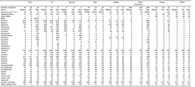
BEIS version 3.61 estimates emissions for 33 volatile organic compounds, carbon monoxide, and nitric oxide. Table 1 shows the complete list of compounds estimated by BEIS with mapping to contemporary gas phase chemical mechanisms SAPRC07T and CB6. BEIS estimates isoprene, 14 unique monoterpene compounds, and total 15
sesquiterpenes. In addition, emissions are estimated for 16 other volatile organic com-pounds and an aggregate group of other unspeciated VOC. All biogenic VOC emis-sions are a function of leaf temperature while only isoprene, methanol, and MBO are a function of both leaf temperature and photosynthetically activated radiation (PAR). All species emissions have small indirect impacts from PAR via the canopy module. 20
Inputs to BEIS include normalized emissions for each vegetation species, gridded vegetation species, temperature, and PAR. Temperature and PAR can be provided from prognostic meteorological models such as WRF or other sources such as satel-lite products (Pinker and Laszlo, 1992; Pinker et al., 2002) or ambient measurements. The BELD 4 database contains vegetation specie information for 275 different vegeta-25
GMDD
8, 8117–8154, 2015Evaluation of improved land use
and canopy representation in
BEIS v3.61
J. O. Bash et al.
Title Page
Abstract Introduction
Conclusions References
Tables Figures
◭ ◮
◭ ◮
Back Close
Full Screen / Esc
Printer-friendly Version
Interactive Discussion
Discussion
P
a
per
|
Discussion
P
a
per
|
Discussion
P
a
per
|
Discussion
P
a
per
|
of crops both irrigated and non-irrigated (40 total). The remaining categories include tree species, much of which are broadleaf (e.g. oak) and needle leaf (e.g. fir) species. A gridded file indicating leaf-on based on the 2009 modeled meteorology, bioseasons file, is also provided as input to BEIS. In the future leaf out and leaf fall dates will be matched with LAI data. However, it is unlikely the current simple leaf-on parameteri-5
zation will impact typical regulatory assessments since elevated O3and PM2.5organic
carbon events often happen outside the spring and fall seasons.
For various sensitivity studies presented here, BEIS 3.14 is applied with BELD 3 vegetation data, WRF temperature, and both WRF and satellite derived estimates of PAR. BEIS 3.61 is applied similarly but with BELD 3 and BELD 4 vegetation data to 10
isolate the impact of the updates to the canopy model. A gridded 0.5 by 0.5◦ resolu-tion satellite estimate of PAR from 2009 was processed to match the model domain specifications and input to both BEIS and MEGAN. The satellite estimates are based on the GEWEX Continental Scale International Project and GEWEX Americas Pre-diction Project Surface Radiation Budget (www.atmos.umd.edu/~srb/gcip/gcipsrb.htm) 15
(Pinker et al., 2002). MEGAN version 2.1 (Guenther et al., 2014, 2012) with version 2011 North America Leaf Area Index and Plant Functional Type (Guenther et al., 2014) was applied with WRF estimated temperature and PAR and also with satellite derived PAR.
2.3 Canopy Model – Leaf temperature update
20
BEIS 3.61 includes a two layer canopy model. Layer structure varies with light inten-sity and solar zenith angle. Both layers of the canopy model include estimates of sunlit and shaded leaf area based on solar zenith angle and light intensity, direct and diffuse solar radiation, and leaf temperature. BEIS 3.14 previously used 2 m temperature to represent canopy temperature for emissions estimation even though BVOC emission 25
ap-GMDD
8, 8117–8154, 2015Evaluation of improved land use
and canopy representation in
BEIS v3.61
J. O. Bash et al.
Title Page
Abstract Introduction
Conclusions References
Tables Figures
◭ ◮
◭ ◮
Back Close
Full Screen / Esc
Printer-friendly Version
Interactive Discussion
Discussion
P
a
per
|
Discussion
P
a
per
|
Discussion
P
a
per
|
Discussion
P
a
per
|
proximate leaf temperature using an energy balance for the sunlit and shaded portion of each canopy layer. Emissions are estimated for sunlit and shaded fractions of the canopy and summed over the two layers for total canopy emissions.
A simple two big leaf (sun and shade) temperature model was developed based on a radiation balance. The leaf radiation balance is solved for both the sun (Eq. 1) and 5
shaded (Eq. 2) leaf sides in each layer. sun leaf
Rabs+IRin−IRout−H−λE+G=0 (1)
shade leaf
Rshade+IRin−IRout−H−λE+G=0, (2)
10
where IRinis the incoming infrared radiation, IRoutis the outgoing infrared radiation,λis the latent heat of evaporation,Esun and Eshade are the latent heat flux from sun and shade leaves respectively,H is the sensible heat flux, andG is the soil heat flux. To maintain the same energy balance as WRF it was assumed thatE scales linearly with sunlit and shaded fractions of the canopy. Note, that conventionallyGis positive when 15
the soil is being heated and negative when the soil is cooling while the sign convention of the other variables are relevant to heating and cooling of the atmosphere.Rabs is the total incoming solar radiation from the meteorological model andRshadeis modeled using the attenuation, scattering and diffuse radiation from Weiss and Norman (1985).
The infrared budget is parameterized as 20
IRin=εatmσTatm4 (3)
IRout=εleafσTleaf4 , (4)
whereεatmand εleaf are the emissivities of the atmosphere and leaf respectively, σis the Stephan Bolzman constant andTatmandTleafare the atmospheric and leaf temper-atures respectively.
GMDD
8, 8117–8154, 2015Evaluation of improved land use
and canopy representation in
BEIS v3.61
J. O. Bash et al.
Title Page
Abstract Introduction
Conclusions References
Tables Figures
◭ ◮
◭ ◮
Back Close
Full Screen / Esc
Printer-friendly Version
Interactive Discussion
Discussion
P
a
per
|
Discussion
P
a
per
|
Discussion
P
a
per
|
Discussion
P
a
per
|
E is parameterized as
E=es(Tleaf)−ea
Rw,leafPatm , (5)
wherees(Tleaf) is the saturation vapor pressure at the leaf,eais the atmospheric vapor pressure,Rw,leafis the resistance to water vapor transport from the leaf to atmosphere andPatmis the atmospheric pressure at the surface.
5
The saturation vapor pressure of the leaf is defined as
es(Tleaf)=ae
b(Tleaf−273.15)
Tleaf−c , (6)
where the empirical coefficients area=611.0 Pa,b=17.67, andc=29.65◦C.
H is parameterized following the WRF Pleim-Xiu (PX) land surface model
(Ska-marock et al., 2008) as 10
H=
ρatmCp P0
Patm
RatmCp
(Tleaf−Tair)
Rh,leaf , (7)
whereρatmis the atmospheric density,Cpis the specific heat of air,P0is the STP pres-sure,Ratm is the gas constant for dry air, andRh,leafis the resistance to heat advection between the atmosphere and leaf.
TheTleaf4 variable and Eq. (6) prevents an analytical solution. Thus the approximation 15
from Campbell and Norman (1998) is used. TheTleaf4 term is simplified as follows:
εleafσTleaf4 ≈εσTatm4 +
ρatmCp P0
Patm
Ratm
C
p
(Tleaf−Tair)
GMDD
8, 8117–8154, 2015Evaluation of improved land use
and canopy representation in
BEIS v3.61
J. O. Bash et al.
Title Page
Abstract Introduction
Conclusions References
Tables Figures
◭ ◮
◭ ◮
Back Close
Full Screen / Esc
Printer-friendly Version
Interactive Discussion
Discussion
P
a
per
|
Discussion
P
a
per
|
Discussion
P
a
per
|
Discussion
P
a
per
|
where Rr,leaf is the atmospheric radiative resistance ∼230 s m−1 (Monteith and Unsworth, 2013).
Equation (6) is then further simplified:
λρatmes(Tleaf)−ea
Rw,leafPatm ≈λS(Tatm)
Tleaf−Tatm
Rw,leaf +λρatm
es(Tatm)−ea
PatmRw,leaf , (9) where
5
S=d es(T)
dT . (10)
Equations (1), (3), (5), (7), (8), and (9) are algebraically combined to estimate the sunlit leaf temperature assuming thatεatm=εleaf.
Tsun,leaf≈Tatm+
Rsun+G−λρatmes(Tatm)−ea
PatmRw,leaf
ρatm
P
0
Patm
RCp
CpR1
h,leaf +
1
Rr,leaf
+λSR1
w,leaf
. (11)
Equations (2), (3), (5), (7), (8), and (9) are combined to estimate the shaded leaf 10
temperature:
Tshade,leaf≈Tatm+
Rshade+G−λρatmes(Tatm)−ea
PatmRw,leaf
ρatm
P
0
Patm
RCp
CpR1
h,leaf +
1
Rr,leaf
+λSR1
w,leaf
. (12)
The sunlit leaf area index, LAISun, is estimated following (Campbell and Norman, 1998)
LAISun=
LAI
Z
0
e−kbe(Ψ)LdL, (13)
GMDD
8, 8117–8154, 2015Evaluation of improved land use
and canopy representation in
BEIS v3.61
J. O. Bash et al.
Title Page
Abstract Introduction
Conclusions References
Tables Figures
◭ ◮
◭ ◮
Back Close
Full Screen / Esc
Printer-friendly Version
Interactive Discussion
Discussion
P
a
per
|
Discussion
P
a
per
|
Discussion
P
a
per
|
Discussion
P
a
per
|
where LAI is the total canopy leaf area index, kbe is the extinction coefficent for di-rect beam incoming solar radiation as a function of the solar zenith angle,Ψfollowing Campbell and Norman (1998). The shaded leaf area index, LAIShade, is then estimated
as follows:
LAIShade=LAI−LAISun. (14)
5
BVOC emission fluxes,Fi, are estimated similar to Guenther et al. (2006) for sunlit and shaded fractions of the canopy
Fi,j =EiγPAR,i,jγT,i,jLAIj, (15)
whereEi is the emission factor or BVOC speciesi,γPAR is the emission activity factor for PAR (currently only applied to isoprene, methanol and MBO), γT is the emission 10
activity factor for leaf temperature following Guenther et al. (1993), andjis the index for sunlit or shaded leaves.γPAR integrates the PAR emissions activity factor of Guenther et al. (1993) for sunlit and shaded layers following Niinemets et al. (2010).
γPAR,i,Sunlit=PARCL
LAISun
Z
0
e−2kddL p
1+α2PAR2e−2kddL
dL (16)
15
γPAR,i,Shaded=PARCL
LAI
Z
LAISun
e−2kddL p
1+α2PAR2e−2kddL
dL, (17)
GMDD
8, 8117–8154, 2015Evaluation of improved land use
and canopy representation in
BEIS v3.61
J. O. Bash et al.
Title Page
Abstract Introduction
Conclusions References
Tables Figures
◭ ◮
◭ ◮
Back Close
Full Screen / Esc
Printer-friendly Version
Interactive Discussion
Discussion
P
a
per
|
Discussion
P
a
per
|
Discussion
P
a
per
|
Discussion
P
a
per
|
2.4 Photochemical model background, inputs, and application
Chemical species are estimated using the Community Multiscale Air-Quality Model (CMAQ) version 5.0.2 (www.cmaq-model.org) photochemical grid model. CMAQ was applied with SAPRC07TB gas phase chemistry (Hutzell et al., 2012), ISORROPIA II in-organic chemistry (Fountoukis and Nenes, 2007), secondary in-organic aerosol treatment 5
(Carlton et al., 2010) and aqueous phase chemistry that oxidizes sulfur, glyoxal, and methyglyoxal (Carlton et al., 2008; Sarwar et al., 2013). The Weather Research and Forecasting (WRF) Advanced Research WRF core (ARW) version 3.3 (Skamarock et al., 2008) was used to generate gridded meteorological inputs for CMAQ and emis-sions models. While not coincident with this study, this WRF configuration compared 10
well with mixing layer height and surface measurements of temperature and winds in central California during the summer of 2010 (Baker et al., 2013). For model per-formance evaluation presented here, model estimates are paired with measurements using the grid cell where the measurement was located. Measurements are paired in time with hourly model estimates with the closest model hour (Simon et al., 2012). 15
The model domain covers central and northern California with 4 km square sized grid cells. The surface to 50 mb is resolved with 34 layers. Layers nearest the surface are most finely resolved with an approximate height of 38 m for layer 1. The modeling period extends from 3 June through 31 July 2009 to be coincident with the BEARPEX field campaign and minimize the influence of initial conditions on model estimates. Ini-20
tial conditions and boundary inflow are from a coarser CMAQ simulation covering the continental United States. Inflow to the coarser simulation is from a global 2009 ap-plication of the GEOS-CHEM (v8-03-02) model (http://acmg.seas.harvard.edu/geos/) (Henderson et al., 2014).
Stationary point sources are based on 2009 specific emissions where available and 25
Ma-GMDD
8, 8117–8154, 2015Evaluation of improved land use
and canopy representation in
BEIS v3.61
J. O. Bash et al.
Title Page
Abstract Introduction
Conclusions References
Tables Figures
◭ ◮
◭ ◮
Back Close
Full Screen / Esc
Printer-friendly Version
Interactive Discussion
Discussion
P
a
per
|
Discussion
P
a
per
|
Discussion
P
a
per
|
Discussion
P
a
per
|
trix Operator Kernel Emissions (SMOKE) model (http://www.cmascenter.org/smoke). Other non-point and commercial marine emissions are based on the 2008 NEI version 2 (http://www.epa.gov/ttn/chief/net/2008inventory.html).
2.5 Field study measurements
Between 15 June and 31 July 2009, the BEARPEX study was conducted to study 5
photochemical reactions and products in areas downwind of urban areas with large biogenic influences. The study was located at a managed ponderosa pine plantation in the foothills of the Sierra Nevada (38.90◦N, 120.63◦W), located near the Univer-sity of California’s Blodgett Research Forest Station. The measurement site was near Georgetown, CA, approximately 75 km from Sacramento, CA. Two research towers 10
housed meteorology and atmospheric composition measurements and inlets during BEARPEX 2009. Meteorological measurements were made on the south, 12.5 m tower, including photosynthetically active radiation (PAR) measured by a LI-COR LI190. The second tower (17.8 m) was located approximately 10 m north of the meteorological tower and housed most of the atmospheric composition measurements. The inlet used 15
to sample BVOCs was located at the top of the north tower, approximately 9 m above the ponderosa pine canopy level. BVOCs including isoprene, monoterpenes, methyl vinyl ketone, and methacrolein were quantified using an online gas chromatograph with a flame ionization detector (GC-FID) (Park et al., 2010, 2011). BVOC samples were collected during the first 30 min of every hour, then subsequently analyzed with 20
the GC-FID.
During June 2010, the CARES study was conducted to study the formation of or-ganic aerosols and the subsequent impacts on climate. The study was composed of two surface monitoring sites: T0 and T1. The T0 was located in Sacramento, CA at the
American River College campus (38.65◦
N, 121.35◦
W), and the T1 site was in Cool, 25
GMDD
8, 8117–8154, 2015Evaluation of improved land use
and canopy representation in
BEIS v3.61
J. O. Bash et al.
Title Page
Abstract Introduction
Conclusions References
Tables Figures
◭ ◮
◭ ◮
Back Close
Full Screen / Esc
Printer-friendly Version
Interactive Discussion
Discussion
P
a
per
|
Discussion
P
a
per
|
Discussion
P
a
per
|
Discussion
P
a
per
|
at the Sacramento (TO) and Cool (T1) CARES ground sites were made with GC-MS and PTRMS, respectively (Zaveri et al., 2012), and sampled via inlets at approximately 10 m above the surface. PTRMS data were reported as 1 s measurements approxi-mately every 30 s. GC-MS data were 10 min collections every 30 min. All observation data was averaged to hourly concentrations before comparison with model estimates. 5
The sunlight leaf temperature in MEGAN 2.1 and the revised canopy model in BEIS 3.61 were evaluated against observations taken in 2008 at the Blackwood Division of the Duke Forest in Orange County, North Carolina, USA (35.97◦
N, 79.09◦
W). De-tails regarding the site (FLUXNET, 2014), measurements, and species composition are available elsewhere (Almand-Hunter et al., 2015). Leaf temperature measurements 10
were taken using an infrared temperature sensor (IRTS-P, Apogee Instruments Inc, Logan, UT) mounted on the grassland tower.
3 Results
3.1 Leaf temperature algorithms compared to observations
The canopy model updates for leaf temperature estimation are evaluated by comparing 15
canopy model output with infrared skin temperature measurements of a grass canopy at the Duke Forest field site in central North Carolina (Fig. 1). BEIS 3.61 canopy model inputs are based on field measurements taken at this location coincident with the skin temperature data collection. The infrared skin temperature measurements do not rep-resent a mean canopy leaf temperature but rather the temperature of the portion of 20
the canopy exposed to the atmosphere. The infrared skin temperature measurement should be warmer than the mean leaf temperature during periods of solar irradiation and cooler during periods of radiative cooling due to the insulating effect of the un-exposed portion of the canopy. Only the estimated un-exposed leaf temperature (Eq. 12) was used in the evaluation to account for this discrepancy between measurements and 25
temper-GMDD
8, 8117–8154, 2015Evaluation of improved land use
and canopy representation in
BEIS v3.61
J. O. Bash et al.
Title Page
Abstract Introduction
Conclusions References
Tables Figures
◭ ◮
◭ ◮
Back Close
Full Screen / Esc
Printer-friendly Version
Interactive Discussion
Discussion
P
a
per
|
Discussion
P
a
per
|
Discussion
P
a
per
|
Discussion
P
a
per
|
ature and difference between leaf and ambient temperature. The average temperature estimated by the BEIS 3.61 canopy model for the top of the canopy compares well with observations (mean bias of 0.3 K and mean error 1.2 K). Top of the canopy leaf tem-perature estimated by MEGAN 2.1 are comparable to BEIS 3.61 and the observations at the Duke Forest site.
5
3.2 Evaluation of the BELD 4 land use data
BELD 4 total forest biomass estimates were evaluated against the independent esti-mates of Blackard et al. (2008). Figure 2 shows the BELD 4 and (Blackard et al., 2008) estimates of forest biomass for this model domain at 4 km resolution. The (Blackard et al., 2008) 250 m grid resolution data set was projected and aggregated to the CMAQ 10
4 km grid resolution projection using rgdal and raster libraries in R (Bivand et al., 2014). The BELD 4 estimates evaluated well against those of (Blackard et al., 2008) with a Pearson’s correlation coefficient of 0.872 (p <0.001) and a mean and median diff er-ence in tree biomass in areas where the NLCD data indicated canopy coverage was −13 kg ha−1
(−32 %) and−0.004 kg ha−1
(0 %) respectively. BELD 4 estimates of forest 15
biomass were greater than those of Blackard et al. (2008) in the densely forested areas in the high Sierras and lower in the lower elevation areas of the domain, primarily in the basin and range areas in the Sacramento valley. The prevalence of the lower elevation areas with lower biomass estimates drives the difference between the forest biomass estimates. The biomass estimates of Blackard et al. (2008) under predicted the full 20
range of the biomass variability with over predictions in areas with low biomass and under predictions in areas of high biomass compared to the FIA tree survey biomass observations. The total biomass estimates presented here have a larger range, 0– 661 kg ha−1versus 0–499 kg ha−1with a median absolute deviation of 2.9 kg ha−1 ver-sus 2.5 kg ha−1
for areas with NLCD canopy coverage. The lower biomass estimates 25
gen-GMDD
8, 8117–8154, 2015Evaluation of improved land use
and canopy representation in
BEIS v3.61
J. O. Bash et al.
Title Page
Abstract Introduction
Conclusions References
Tables Figures
◭ ◮
◭ ◮
Back Close
Full Screen / Esc
Printer-friendly Version
Interactive Discussion
Discussion
P
a
per
|
Discussion
P
a
per
|
Discussion
P
a
per
|
Discussion
P
a
per
|
eral underestimation of 2001 NLCD canopy fraction product (Nowak and Greenfield, 2012).
There are currently no databases to quantitatively evaluate the fractional tree species data coverage developed here. However the species range maps of Critchfield and Little (1966) and Little Jr. (1971, 1976) can be used for a qualitative evaluation. The 5
tree species that constituted the largest fraction of biomass observations in the FIA data base generally fell within the tree species range maps (Fig. 3). Note that the maps represent a binary distribution of the tree species natural range and the BELD 4 estimates represent a gradient of species density. Species that did not constitute a large fraction in FIA observations typically had a much smaller estimated spatial 10
range than indicated by the range maps. This could partially be due to the criteria, e.g. tree height greater than 5 m, etc., for trees carried over from the NLCD classification scheme or due to sparse sampling of these tree species in the FIA data base due to the species scarcity. However, these species likely represent a small fraction of the forest coverage in the domain and a small fraction of the domain wide BVOC emissions. Also, 15
it is possible that tree coverage has changed in California since the 1970s when the trees were surveyed due to urban planning, plantations, fire, forest growth and climate change.
3.3 Describing changes in modeled BVOC estimates in Northern California
Biogenic VOC emissions estimated with BEIS using the new canopy model (BEIS 3.61) 20
and updated vegetation data (BELD 4) are shown for the northern California region in Fig. 4. A similar Figure of spatial biogenic emissions estimated with BEIS 3.14 and BELD 3 are shown in Fig. 5. In this model domain, isoprene emissions are highest in the foothills of the Sierra Nevada where high emitting isoprene vegetation (e.g. oak trees) are located. Monoterpene emissions are highest in the Sierra Nevada Mountains 25
GMDD
8, 8117–8154, 2015Evaluation of improved land use
and canopy representation in
BEIS v3.61
J. O. Bash et al.
Title Page
Abstract Introduction
Conclusions References
Tables Figures
◭ ◮
◭ ◮
Back Close
Full Screen / Esc
Printer-friendly Version
Interactive Discussion
Discussion
P
a
per
|
Discussion
P
a
per
|
Discussion
P
a
per
|
Discussion
P
a
per
|
biogenic VOC emissions show similar spatial patterns as isoprene or monoterpenes (Fig. 4).
The fractional coverage of oak (high isoprene emitting species) and needle leaf trees (high monoterpene emitting species) are shown using BELD 3 and BELD 4 in Fig. S2. The BELD 4 representation shows a higher intensity of fractional coverage in much of 5
the Sierra Nevada as county level information is allocated more spatially explicitly than in BELD 3. Smearing out vegetation coverage, as in BELD 3, will lead to lower emis-sions estimates where narrow features such as the band of oak trees in the western Sierra Nevada foothills exist and over predictions in areas that get allocated vegetation that does not exist in that area. Changes in oak and needle leaf fractional coverage 10
between BELD 3 and BELD 4 are notable for both the Cool and Blodgett Forest sites meaning the observation data available at these locations is useful for evaluating the methodology used to generate BELD 4 (Fig. S2).
The updated leaf canopy module increases biogenic VOC emissions throughout Cal-ifornia (Fig. 5). The changes to the vegetation input data show increases and decreases 15
in isoprene and monoterpene emissions related to changing spatial allocation of high emitting vegetation species and changes to leaf area estimates. Sesquiterpene emis-sions generally decrease due to the changes in landuse and vegetation for this region (Fig. 5). The new vegetation allocation approach employed here for BELD 4 provides more detailed sub-County level representation of emitting species compared to BELD 20
3 and those changes are reflected in biogenic VOC emissions differences.
3.4 CMAQ estimates compared with CARES and BEARPEX measurements
The most recent publicly available version of BEIS (version 3.14) and BELD 3 veg-etation input were used to provide biogenic emissions for a 4 km CMAQ simulation covering northern and central California for the period of time coincident with the 2009 25
GMDD
8, 8117–8154, 2015Evaluation of improved land use
and canopy representation in
BEIS v3.61
J. O. Bash et al.
Title Page
Abstract Introduction
Conclusions References
Tables Figures
◭ ◮
◭ ◮
Back Close
Full Screen / Esc
Printer-friendly Version
Interactive Discussion
Discussion
P
a
per
|
Discussion
P
a
per
|
Discussion
P
a
per
|
Discussion
P
a
per
|
satellite derived PAR as input to BEIS rather than WRF estimated solar radiation. The MEGAN 2.1 model was also run using WRF and satellite estimates of PAR for the same domain and period.
Temperature and solar radiation used for the biogenic emissions models were com-pared to measurements at these field sites (Sacramento, Cool, and Blodgett Forest) 5
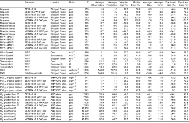
to determine how meteorological inputs may bias model estimated BVOC. WRF model evaluation against meteorological variables is summarized in Table 3. The WRF model does well at capturing daytime high temperatures at Blodgett Forest and slightly over-estimates daily peak PAR. Daytime minimum temperatures at Blodgett Forest are largely overestimated by WRF. Temperature maximums and minimums are well char-10
acterized at Sacramento and Cool. The satellite estimated PAR underestimates the ground measurements at Blodgett Forest on certain days but does better at capturing daytime peaks than WRF. In general, meteorological model performance at Blodgett Forest should result in overestimated emissions of isoprene and monoterpenes due to model overestimates in PAR and nighttime ambient temperature.
15
Field study measurements of isoprene and monoterpenes taken in 2010 at Sacra-mento and Cool and 2009 at Blodgett Forest provide an opportunity to better under-stand if the changes to BEIS and BELD better reflect the biogenic VOC gradient seen over these sites. Figure 6 shows the observed distribution of isoprene concentrations at Sacramento and Cool from 2010, Blodgett Forest in 2009, and model estimates from 20
2009 for the baseline CMAQ/BEIS simulation (BEIS 3.14 and BELD 3), canopy model updates (BEIS 3.61), vegetation data updates (BELD 4), and using satellite PAR with all formulation and other input data updates. Measured isoprene concentrations are lowest in Sacramento and highest at Cool where a high density of Oak trees exist. The baseline simulation predicts the highest isoprene at Blodgett Forest rather than Cool, 25
GMDD
8, 8117–8154, 2015Evaluation of improved land use
and canopy representation in
BEIS v3.61
J. O. Bash et al.
Title Page
Abstract Introduction
Conclusions References
Tables Figures
◭ ◮
◭ ◮
Back Close
Full Screen / Esc
Printer-friendly Version
Interactive Discussion
Discussion
P
a
per
|
Discussion
P
a
per
|
Discussion
P
a
per
|
Discussion
P
a
per
|
Measured monoterpenes are highest at Blodgett Forest and lowest at Sacramento (Fig. 7). The baseline model captured this gradient but notably overestimated monoter-penes at Cool. When BELD 4 is used as input the modeling system compares much closer to observations at Cool and begins to slightly underestimate at Blodgett For-est. The use of satellite PAR rather than solar radiation estimated by WRF does little 5
to change model performance of isoprene. Monoterpenes are not directly sensitive to PAR input and change little due to indirect use of PAR in the canopy model.
The MEGAN 2.1 model generally captures the gradient in observations between sites for isoprene and monoterpenes, but predicts much higher isoprene concentra-tions at each site compared to observaconcentra-tions (see Fig. 6). This is consistent with other 10
studies comparing MEGAN 2.1 isoprene flux with measurements in the Sierra Nevada of northern California (Misztal et al., 2014) and also with modeling systems using MEGAN 2.1 isoprene emissions compared with ambient isoprene concentrations in Texas (Kota et al., 2015) and southern Missouri (Carlton and Baker, 2011). Using the MEGAN model estimates of monoterpenes resulted in overestimates at Cool and un-15
derestimates at Blodgett Forest (Fig. 7). Estimates of isoprene using MEGAN improved when using satellite PAR as input rather than WRF solar radiation. This is consistent with similar evaluation in other parts of the United States (Carlton and Baker, 2011). The use of satellite PAR with MEGAN exacerbated monoterpene overestimates at Cool and increased model estimates at Blodgett Forest reducing the model underestimate. 20
First generation oxidation products of isoprene (methacrolein and methyl vinyl ketones) were also measured at Blodgett Forest in 2009. Model performance is similar to iso-prene where BEIS estimates compare favorably with measurements and MEGAN 2.1 emissions result in notable overestimates (Fig. S3) similar to previous studies (Kota et al., 2015). Methacrolein can further react in the atmosphere to form methacryloyl per-25
GMDD
8, 8117–8154, 2015Evaluation of improved land use
and canopy representation in
BEIS v3.61
J. O. Bash et al.
Title Page
Abstract Introduction
Conclusions References
Tables Figures
◭ ◮
◭ ◮
Back Close
Full Screen / Esc
Printer-friendly Version
Interactive Discussion
Discussion
P
a
per
|
Discussion
P
a
per
|
Discussion
P
a
per
|
Discussion
P
a
per
|
MEGAN. Model performance for isoprene propagates through secondary reactions and could lead to similar over or under estimates of SOA.
4 Future direction
The updated biomass and tree species vegetation characterization in BELD would benefit from additional evaluation for other parts of the conterminous United States. 5
It is critically important to evaluate biogenic emissions models with field experiments designed for biogenic model evaluation or those that provide robust measurements of key biogenic VOC species such as those used for this assessment. Future work is planned to evaluate BEIS against a larger field study in California designed for biogenic emissions model evaluation (2011 California Airborne BVOC Emission Research in 10
Natural Ecosystem Transects; CABERNET) (Karl et al., 2013; Misztal et al., 2014) and also with a field study done in the southeast United States during the summer of 2013 (Southern Oxidant and Aerosol Study; SOAS). Evaluation of the model in urban areas would be useful although little field data exists for urban areas making this type of assessment difficult.
15
Code availability
BEIS 3.61 code is available upon request prior to the public release of CMAQ v5.1 and available now in SMOKE 3.6.5 (https://www.cmascenter.org/smoke/). Please contact Jesse Bash at [email protected] for more information. Additional model output, comparison with measurements and formulas used for data pairing are provided in the 20
Supplement.
GMDD
8, 8117–8154, 2015Evaluation of improved land use
and canopy representation in
BEIS v3.61
J. O. Bash et al.
Title Page
Abstract Introduction
Conclusions References
Tables Figures
◭ ◮
◭ ◮
Back Close
Full Screen / Esc
Printer-friendly Version
Interactive Discussion
Discussion
P
a
per
|
Discussion
P
a
per
|
Discussion
P
a
per
|
Discussion
P
a
per
|
Acknowledgements. The authors would like to acknowledge Lara Reynolds, Charles Chang, Allan Beidler, Chris Allen, James Beidler, Chris Geron, and Alex Guenther. Jeong-Hoo Park and Allen H. Goldstein from the University of California, Berkeley. Berk Knighton and Cody Floerchinger from the University of Montana. Gunnar Shade and Chang Hyoun from Texas A&M University. Thomas Jobson from Washington State University. Although this work was 5
reviewed by EPA and approved for publication, it may not necessarily reflect official Agency
policy.
References
Almand-Hunter, B. B., Walker, J. T., Masson, N. P., Hafford, L., and Hannigan, M. P.:
Develop-ment and validation of inexpensive, automated, dynamic flux chambers, Atmos. Meas. Tech., 10
8, 267–280, doi:10.5194/amt-8-267-2015, 2015.
Baker, K. R., Misenis, C., Obland, M. D., Ferrare, R. A., Scarino, A. J., and Kelly, J. T.: Evaluation of surface and upper air fine scale WRF meteorological modeling of the May and June 2010 CalNex period in California, Atmos. Environ., 80, 299–309, doi:10.1016/j.atmosenv.2013.08.006, 2013.
15
Beaver, M. R., Clair, J. M. St., Paulot, F., Spencer, K. M., Crounse, J. D., LaFranchi, B. W., Min, K. E., Pusede, S. E., Wooldridge, P. J., Schade, G. W., Park, C., Cohen, R. C., and Wennberg, P. O.: Importance of biogenic precursors to the budget of organic nitrates: observations of multifunctional organic nitrates by CIMS and TD-LIF during BEARPEX 2009, Atmos. Chem. Phys., 12, 5773–5785, doi:10.5194/acp-12-5773-2012, 2012.
20
Bell, M. L., McDermott, A., Zeger, S. L., Samet, J. M., and Dominici, F.: Ozone and short-term mortality in 95 US urban communities, 1987–2000, Jama-Journal of the American Medical Association, 292, 2372–2378, 10.1001/jama.292.19.2372, 2004.
Bivand, R., Keitt, T., Rowlingson, B., Pebesma, E., Summer, M., Hijmans, R., and Rouault, E.: Package ’rgdal’: Bindings for the Geosptail Data Abstraction Library, available at: http: 25
//cran.r-project.org/web/packages/rgdal/rgdal.pdf, last access: 8 August 2014.
GMDD
8, 8117–8154, 2015Evaluation of improved land use
and canopy representation in
BEIS v3.61
J. O. Bash et al.
Title Page
Abstract Introduction
Conclusions References
Tables Figures
◭ ◮
◭ ◮
Back Close
Full Screen / Esc
Printer-friendly Version
Interactive Discussion
Discussion
P
a
per
|
Discussion
P
a
per
|
Discussion
P
a
per
|
Discussion
P
a
per
|
Byun, D. and Schere, K. L.: Review of the governing equations, computational algorithms, and other components of the models-3 Community Multiscale Air Quality (CMAQ) modeling sys-tem, Appl. Mech. Rev., 59, 51–77, doi:10.1115/1.2128636, 2006.
Campbell, G. S. and Norman, J. M.: An introduction to environmental biophysics, Springer, 1998.
5
Carlton, A. G. and Baker, K. R.: Photochemical Modeling of the Ozark Isoprene Volcano: MEGAN, BEIS, and Their Impacts on Air Quality Predictions, Environ. Sci. Technol., 45, 4438–4445, doi:10.1021/es200050x, 2011.
Carlton, A. G., Turpin, B. J., Altieri, K. E., Seitzinger, S. P., Mathur, R., Roselle, S. J., and Weber, R. J.: CMAQ model performance enhanced when in-cloud SOA is included: comparisons of 10
OC predictions with measurements, Environ. Sci. Technol., 42, 8798–8802, 2008.
Carlton, A. G., Wiedinmyer, C., and Kroll, J. H.: A review of Secondary Organic Aerosol (SOA) formation from isoprene, Atmos. Chem. Phys., 9, 4987–5005, doi:10.5194/acp-9-4987-2009, 2009.
Carlton, A. G., Bhave, P. V., Napelenok, S. L., Edney, E. O., Sarwar, G., Pinder, R. W., Pouliot, 15
G. A., and Houyoux, M.: Treatment of secondary organic aerosol in CMAQv4.7, Environ. Sci. Technol., 44, 8553–8560, 2010.
Chameides, W. L., Lindsay, R. W., Richardson, J., and Kiang, C. S.: The role of biogenic huydro-carbons in urban photochemical smog – Atlanta as a case-study, Science, 241, 1473–1475, 1988.
20
Chojnacky, D. C., Heath, L. S., and Jenkins, J. C.: Updated generalized biomass equations for North American tree species, Forestry, 87, 129–151, 2014.
Critchfield, W. B. and Little, E. L.: Geographic distribution of the pines of the world, US Depart-ment of Agriculture, Forest Service, 1966.
Dreyfus, G. B., Schade, G. W., and Goldstein, A. H.: Observational constraints on the contri-25
bution of isoprene oxidation to ozone production on the western slope of the Sierra Nevada, California, J. Geophys. Res.-Atmos., 107, ACH 1-1–ACH 1-17, 2002.
Fann, N., Fulcher, C. M., and Baker, K.: The Recent and Future Health Burden of Air Pollution Apportioned Across US Sectors, Environ. Sci. Technol., 47, 3580–3589, 2013.
FLUXNET: Duke Fores Open Field, available at: http://fluxnet.ornl.gov/site/867, last access: 30
8 August 2014.
GMDD
8, 8117–8154, 2015Evaluation of improved land use
and canopy representation in
BEIS v3.61
J. O. Bash et al.
Title Page
Abstract Introduction
Conclusions References
Tables Figures
◭ ◮
◭ ◮
Back Close
Full Screen / Esc
Printer-friendly Version
Interactive Discussion
Discussion
P
a
per
|
Discussion
P
a
per
|
Discussion
P
a
per
|
Discussion
P
a
per
|
J. O.: Incremental testing of the Community Multiscale Air Quality (CMAQ) modeling system version 4.7, Geosci. Model Dev., 3, 205–226, doi:10.5194/gmd-3-205-2010, 2010.
Fountoukis, C. and Nenes, A.: ISORROPIA II: a computationally efficient thermodynamic
equi-librium model for K+–Ca2+–Mg2+–NH+4–Na+–SO2−
4 –NO
−
3–Cl
−–H
2O aerosols, Atmos. Chem.
Phys., 7, 4639–4659, doi:10.5194/acp-7-4639-2007, 2007. 5
Guenther, A., Duhl, T., Sakulyanontvittaya, T., and Wang, X.: MEGAN version 2.10 User’s Guide, available at: http://lar.wsu.edu/megan/guides.html, last access: 25 August 2014. Guenther, A. B., Jiang, X., Heald, C. L., Sakulyanontvittaya, T., Duhl, T., Emmons, L. K.,
and Wang, X.: The Model of Emissions of Gases and Aerosols from Nature version 2.1 (MEGAN2.1): an extended and updated framework for modeling biogenic emissions, Geosci. 10
Model Dev., 5, 1471–1492, doi:10.5194/gmd-5-1471-2012, 2012.
Henderson, B. H., Akhtar, F., Pye, H. O. T., Napelenok, S. L., and Hutzell, W. T.: A database and tool for boundary conditions for regional air quality modeling: description and evaluation, Geosci. Model Dev., 7, 339–360, doi:10.5194/gmd-7-339-2014, 2014.
Homer, C., Huang, C., Yang, L., Wylie, B. K., and Coan, M.: Development of a 2001 national 15
land-cover database for the United States, 2004.
Hutzell, W. T., Luecken, D. J., Appel, K. W., and Carter, W. P. L.: Interpreting predictions from the SAPRC07 mechanism based on regional and continental simulations, Atmos. Environ., 46, 417–429, doi:10.1016/j.atmosenv.2011.09.030, 2012.
Jenkins, J. C., Chojnacky, D. C., Heath, L. S., and Birdsey, R. A.: National-scale biomass esti-20
mators for United States tree species, Forest Sci., 49, 12–35, 2003.
Karl, T., Misztal, P., Jonsson, H., Shertz, S., Goldstein, A., and Guenther, A.: Airborne Flux Measurements of BVOCs above Californian Oak Forests: Experimental Investigation of Sur-face and Entrainment Fluxes, OH Densities, and Damköhler Numbers, J. Atmos. Sci., 70, 3277–3287, 2013.
25
Kelly, J. T., Baker, K. R., Nowak, J. B., Murphy, J. G., Markovic, M. Z., VandenBoer, T. C., Ellis, R. A., Neuman, J. A., Weber, R. J., and Roberts, J. M.: Fine-scale simulation of ammonium and nitrate over the South Coast Air Basin and San Joaquin Valley of California during CalNex-2010, J. Geophys. Res.-Atmos., 119, 3600–3614, 2014.
Kinnee, E., Geron, C., and Pierce, T.: United States land use inventory for estimating biogenic 30
GMDD
8, 8117–8154, 2015Evaluation of improved land use
and canopy representation in
BEIS v3.61
J. O. Bash et al.
Title Page
Abstract Introduction
Conclusions References
Tables Figures
◭ ◮
◭ ◮
Back Close
Full Screen / Esc
Printer-friendly Version
Interactive Discussion
Discussion
P
a
per
|
Discussion
P
a
per
|
Discussion
P
a
per
|
Discussion
P
a
per
|
Kota, S. H., Schade, G., Estes, M., Boyer, D., and Ying, Q.: Evaluation of MEGAN predicted biogenic isoprene emissions at urban locations in Southeast Texas, Atmos. Environ., 110, 54–64, doi:10.1016/j.atmosenv.2015.03.027, 2015.
Kwok, R., Napelenok, S., and Baker, K.: Implementation and evaluation of PM<sub>2.5<
/sub>source contribution analysis in a photochemical model, Atmos. Environ., 80, 398–407,
5
2013.
Lefohn, A. S., Emery, C., Shadwick, D., Wernli, H., Jung, J., and Oltmans, S. J.: Estimates of background surface ozone concentrations in the United States based on model-derived source apportionment, Atmos. Environ., 84, 275–288, doi:10.1016/j.atmosenv.2013.11.033, 2014.
10
Little Jr., E. L.: Atlas of United States trees. Volume 1. Conifers and important hardwoods. Miscellaneous publication 1146, US Department of Agriculture, Forest Service, Washington, DC, 1971.
Little Jr., E. L.: Atlas of United States trees. Volume 3. Minor wesern hardwood. Miscellaneous publication 1314, US Department of Agriculture, Forest Service, Washington, DC, 1976. 15
Misztal, P. K., Karl, T., Weber, R., Jonsson, H. H., Guenther, A. B., and Goldstein, A. H.: Airborne flux measurements of biogenic isoprene over California, Atmos. Chem. Phys., 14, 10631– 10647, doi:10.5194/acp-14-10631-2014, 2014.
Monteith, J. and Unsworth, M.: Principles of Environmental Physics: Plants, Animals, and the Atmosphere, Academic Press, 2013.
20
Niinemets, Ü., Arneth, A., Kuhn, U., Monson, R. K., Peñuelas, J., and Staudt, M.: The emis-sion factor of volatile isoprenoids: stress, acclimation, and developmental responses, Bio-geosciences, 7, 2203–2223, doi:10.5194/bg-7-2203-2010, 2010.
Nowak, D. J. and Greenfield, E. J.: Tree and impervious cover in the United States, Landscape Urban Plan., 107, 21–30, 2012.
25
O’Connell, B., LaPoint, E., Turner, J., Ridley, T., Boyer, D., Wilson, A., Waddell, K., and Conkling, B.: The Forest Inventory and Analysis Database: Database Description and Users Manual Version 5.1. 2 for Phase 2, USDA Forest Service, 2012.
Park, C., Schade, G. W., and Boedeker, I.: Flux measurements of volatile organic compounds by the relaxed eddy accumulation method combined with a GC-FID system in urban Houston, 30
GMDD
8, 8117–8154, 2015Evaluation of improved land use
and canopy representation in
BEIS v3.61
J. O. Bash et al.
Title Page
Abstract Introduction
Conclusions References
Tables Figures
◭ ◮
◭ ◮
Back Close
Full Screen / Esc
Printer-friendly Version
Interactive Discussion
Discussion
P
a
per
|
Discussion
P
a
per
|
Discussion
P
a
per
|
Discussion
P
a
per
|
Park, C., Schade, G. W., and Boedeker, I.: Characteristics of the flux of isoprene and its oxidation products in an urban area, J. Geophys. Res.-Atmos., 116, D21303, doi:10.1029/2011JD015856, 2011.
Pierce, T. E. and Waldruff, P. S.: PC-BEIS: A personal computer version of the biogenic
emis-sions inventory system, J. Air Waste Manage. Assoc., 41, 937–941, 1991. 5
Pinker, R. T. and Laszlo, I.: Global Distribution of Photosynthetically Active Radiation as Ob-served from Satellites, J. Climate, 5, 56–65, 1992.
Pinker, R. T., Laszlo, I., Tarpley, J. D., and Mitchell, K.: Geostationary satellite parameters for surface energy balance, Earth’s Atmosphere, Ocean Surface Studies, 30, 2427–2432, 2002.
Pope, C. A. and Dockery, D. W.: Health effects of fine particulate air pollution: Lines that connect,
10
J. Air Waste Manage. Asso., 56, 709–742, 2006.
Pope III, C. A., Muhlestein, J. B., May, H. T., Renlund, D. G., Anderson, J. L., and Horne, B. D.: Ischemic heart disease events triggered by short-term exposure to fine particulate air pollution, Circulation, 114, 2443–2448, doi:10.1161/circulationaha.106.636977, 2006. Sakulyanontvittaya, T., Duhl, T., Wiedinmyer, C., Helmig, D., Matsunaga, S., Potosnak, M., Mil-15
ford, J., and Guenther, A.: Monoterpene and sesquiterpene emission estimates for the United States, Environ. Sci. Technol., 42, 1623–1629, 2008.
Sarwar, G., Fahey, K., Kwok, R., Gilliam, R. C., Roselle, S. J., Mathur, R., Xue, J., Yu, J., and Carter, W. P. L.: Potential impacts of two SO2 oxidation pathways on regional sulfate concentrations: Aqueous-phase oxidation by NO2 and gas-phase oxidation by Stabilized 20
Criegee Intermediates, Atmos. Environ., 68, 186–197, doi:10.1016/j.atmosenv.2012.11.036, 2013.
Simon, H., Baker, K. R., and Phillips, S.: Compilation and interpretation of photochemical model performance statistics published between 2006 and 2012, Atmos. Environ., 61, 124–139, 2012.
25
Simon, H., Baker, K. R., Akhtar, F., Napelenok, S. L., Possiel, N., Wells, B., and Timin, B.: A Di-rect sensitivity approach to predict hourly ozone resulting from compliance with the National Ambient Air Quality Standard, Environ. Sci. Technol., 47, 2304–2313, 2013.
Skamarock, W. C., Klemp, J. B., Dudhia, J., Gill, D. O., Barker, D. M., Duda, M. G., Huang, X., Wang, W., and Powers, J. G.: A description of the Advanced Reserch WRF version 3., NCAR 30
GMDD
8, 8117–8154, 2015Evaluation of improved land use
and canopy representation in
BEIS v3.61
J. O. Bash et al.
Title Page
Abstract Introduction
Conclusions References
Tables Figures
◭ ◮
◭ ◮
Back Close
Full Screen / Esc
Printer-friendly Version
Interactive Discussion
Discussion
P
a
per
|
Discussion
P
a
per
|
Discussion
P
a
per
|
Discussion
P
a
per
|
US Environmental Protection Agency: Regulatory Impact Analysis for the Proposed Federal Transport Rule, available at: http://www.epa.gov/ttn/ecas/regdata/RIAs/proposaltrri_final.pdf, last access: 12 December 2014., Docket ID No. EPA-HQ-OAR-2009-0491, 2010.
US Environmental Protection Agency: Air Quality Modeling Technical Support Document: Heavy-Duty Vehicle Greenhouse Gas Emission Standards Final Rule (EPA-454/R-11-004), 5
EPA-454/R-11-004, EPA-454/R-11-004, edited by: EPA-454/R-11-004, Research Triangle Park, North Carolina, 2011.
US Environmental Protection Agency: Air Quality Modeling Technical Support Document for the Regulatory Impact Analysis for the Revisions to the National Ambient Air Quality Standards
for Particulate Matter, Office of Air Quality Planning and Standards, Research Triangle Park,
10
North Carolina, 2012.
Warneke, C., de Gouw, J. A., Del Negro, L., Brioude, J., McKeen, S., Stark, H., Kuster, W. C., Goldan, P. D., Trainer, M., Fehsenfeld, F. C., Wiedinmyer, C., Guenther, A. B., Hansel, A., Wisthaler, A., Atlas, E., Holloway, J. S., Ryerson, T. B., Peischl, J., Huey, L. G., and Hanks, A. T. C.: Biogenic emission measurement and inventories determination of biogenic emissions 15
in the eastern United States and Texas and comparison with biogenic emission inventories, J. Geophys. Res.-Atmos., 115, D00F18, doi:10.1029/2009jd012445, 2010.
Weiss, A. and Norman, J.: Partitioning solar radiation into direct and diffuse, visible and
near-infrared components, Agr. Forest Meteorol., 34, 205–213, 1985.
Wiedinmyer, C., Greenberg, J., Guenther, A., Hopkins, B., Baker, K., Geron, C., Palmer, P. 20
I., Long, B. P., Turner, J. R., Petron, G., Harley, P., Pierce, T. E., Lamb, B., Westberg, H., Baugh, W., Koerber, M., and Janssen, M.: Ozarks Isoprene Experiment (OZIE): Measure-ments and modeling of the “isoprene volcano”, J. Geophys. Res.-Atmos., 110, D18307, doi:10.1029/2005jd005800, 2005.
Worton, D. R., Surratt, J. D., LaFranchi, B. W., Chan, A. W. H., Zhao, Y., Weber, R. J., Park, 25
J.-H., Gilman, J. B., de Gouw, J., Park, C., Schade, G., Beaver, M., Clair, J. M. S., Crounse, J., Wennberg, P., Wolfe, G. M., Harrold, S., Thornton, J. A., Farmer, D. K., Docherty, K. S., Cubison, M. J., Jimenez, J.-L., Frossard, A. A., Russell, L. M., Kristensen, K., Glasius, M., Mao, J., Ren, X., Brune, W., Browne, E. C., Pusede, S. E., Cohen, R. C., Seinfeld, J. H., and Goldstein, A. H.: Observational Insights into Aerosol Formation from Isoprene, Environ. Sci. 30
Technol., 47, 11403–11413, doi:10.1021/es4011064, 2013.