www.atmos-chem-phys.net/13/5873/2013/ doi:10.5194/acp-13-5873-2013
© Author(s) 2013. CC Attribution 3.0 License.
Atmospheric
Chemistry
and Physics
Geoscientiic
Geoscientiic
Geoscientiic
Geoscientiic
Modeling air pollution in Lebanon: evaluation at a suburban site in
Beirut during summer
A. Waked1,2, C. Seigneur1, F. Couvidat1, Y. Kim1, K. Sartelet1, C. Afif2, A. Borbon3, P. Formenti3, and S. Sauvage4
1CEREA, Joint Laboratory ´Ecole des Ponts ParisTech/EDF R&D, Universit´e Paris-Est, Champs-sur-Marne, France 2Centre d’Analyses et de Recherche, Faculty of Sciences, Universit´e Saint-Joseph, Beirut, Lebanon
3LISA, CNRS UMR7583, Universit´e Paris-Est Cr´eteil and Universit´e Paris Diderot, Institut Pierre-Simon Laplace, Cr´eteil, France
4Ecole des Mines de Douai, D´epartement Chimie Environnement, 59508 Douai, France
Correspondence to:A. Waked ([email protected], [email protected]) and C. Seigneur([email protected]) Received: 21 August 2012 – Published in Atmos. Chem. Phys. Discuss.: 16 November 2012
Revised: 10 April 2013 – Accepted: 17 May 2013 – Published: 17 June 2013
Abstract. Beirut, the capital of Lebanon, which is located
on the eastern shore of the Mediterranean basin, experiences high air pollution episodes. Annual average concentrations of coarse and fine particulate matter (PM2.5)as well as nitrogen oxides (NOx)often exceed the World Health Organization (WHO) guidelines. Therefore, improving air quality in this region is essential. The Polyphemus/Polair3D modeling sys-tem is used here to investigate air pollution episodes in Beirut during 2 to 18 July 2011. The modeling domain covers two nested grids of 1 and 5 km horizontal resolution over greater Beirut and Lebanon, respectively. The anthropogenic emis-sion inventory was developed earlier (Waked et al., 2012). The Weather and Research Forecasting (WRF) model is used to generate the meteorological fields and the Model of Emis-sions of Gases and Aerosols from Nature (MEGAN) is used for biogenic emissions. The results of the study are compared to measurements from a field campaign conducted in the sub-urb of Beirut during 2–18 July 2011. The model reproduces satisfactorily the concentrations of most gaseous pollutants, the total mass of PM2.5as well as PM2.5elemental carbon (EC), organic carbon (OC), and sulfate. Ozone concentra-tions are overestimated and it appears that this overestima-tion results mainly from the boundary condioverestima-tions.
1 Introduction
result, air pollution in this region needs to be investigated, monitored, and reduced. Lebanon, a small developing coun-try in the Middle East region, located on the eastern shore of the Mediterranean Sea, experiences high pollution episodes due to local emissions because of a growing population, es-pecially in urban areas, the absence of any public transport system (MoE, 2005), steady winds from eastern Europe and Saharan dust storms from the desert (Saliba et al., 2007). Therefore, the country represents a good case study for in-vestigating air pollution in the region. The few measurements conducted in Beirut, the capital city of Lebanon, revealed high levels of nitrogen dioxide (NO2)with an annual aver-age concentration of 66 µg m−3 (Afif et al., 2009) and high levels of particulate matter, PM10 and PM2.5, with annual concentrations of 64 and 20 µg m−3, respectively (Massoud et al., 2011). The levels exceed World Health Organization (WHO) guideline values of 40 µg m−3 for NO
2and 20 and 10 µg m−3for PM
10and PM2.5, respectively. Although these measurements provide valuable information on air pollution, they are scarce and limited to a few areas. Therefore, the use of chemical-transport models (CTM) is essential for un-derstanding the spatio-temporal distribution of gaseous and particulate pollutants in the region. Previous studies have fo-cused on simulating the distribution of O3 over this region using regional CTM. The EMAC chemistry general circu-lation model (Roeckner et al., 2006) was used to investi-gate O3 levels in the Persian gulf region (Leleiveld et al., 2009) and a fully coupled on-line model (WRF-Chem ver-sion 3.3.1) (Grell et al., 2005) was used for the Arabian Peninsula (Smoydzin et al., 2012). However, no modeling study has yet been conducted for Lebanon or its capital city Beirut. In this study, the WRF-ARW version 3.3 meteorolog-ical model (Skamarock et al., 2008) is used with the Polyphe-mus/Polair3D CTM (Mallet et al., 2007; Sartelet et al., 2007) to investigate air pollution in Beirut as well as in Lebanon from 2 to 18 July 2011. WRF has been evaluated against ob-servations in many regions (Borge et al., 2008; Carvalho et al., 2012; Molders, 2008) but, to our knowledge, has never been applied to Lebanon. The Polyphemus/Polair3D CTM has been evaluated over Europe (Sartelet et al., 2007, 2012; Couvidat et al., 2012), Asia (Sartelet et al., 2008), and North America (Sartelet et al., 2012), but not in the Middle East re-gion. This study aims to investigate air pollution in Beirut in July 2011 via meteorological and air quality modeling. The evaluation of WRF and Polyphemus/Polair3D in this region is essential prior to the use of such models for future air qual-ity studies.
The methodology and the model configurations for WRF and Polyphemus/Polair3D are described in Sect. 2. The eval-uation results for the meteorological and chemical simula-tions against observasimula-tions are presented and discussed in Sects. 3 and 4, respectively. Conclusions and future prospects are provided in Sect. 5.
2 Method
2.1 Modeling domains
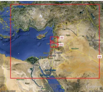
For meteorological modeling, three modeling domains were set on a latitude-longitude projection. A mother domain (D3) with 25 km horizontal resolution covering the Middle East region, as well as some parts of eastern Europe, northern Africa and the Mediterranean Sea, and two nested domains with 5 km resolution for Lebanon (D2) and 1 km resolution for Beirut and its suburbs (D1) were adopted. The two nested domains D1 and D2 are used for the air quality model simu-lations. The nested mother domain (D3) was not used in the air quality model simulations due to the lack of an emission inventory at that resolution over the Middle East region.
2.2 Episode selection and observational data set
2
Fig. 1.The modeling domains D1, D2 and D3 used in this study.
et al., 2010), for organic aerosols using a gas chromatog-raphy coupled to a mass spectrometry (GC/MS) technique, and for inorganic aerosols using an ion chromatography (IC) technique. The model simulation results are compared with those measurements to evaluate the ability of the model to reproduce major chemical components of photochemical air pollution in Beirut.
2.3 Meteorological modeling
WRF-ARW was used to generate the meteorological fields using a two-way nesting approach with a vertical structure of 24 layers covering the whole troposphere. Initial and bound-ary conditions were driven by the National Centers for En-vironmental Prediction (NCEP) global tropospheric analyses with 1◦×1◦spatial resolution and 6 h temporal resolution. Topography and land use were interpolated from the United States Geological Survey (USGS) global land covers with the appropriate spatial resolution for each domain.
Physical parameterizations used in the model include the Kessler cloud microphysics scheme (Kessler, 1969), the Rapid Radiation Transfer Model (RRTM) long-wave radia-tion scheme (Mlawer et al., 1997), the Goddard NASA short-wave scheme (Chou and Suarez, 1994), the Grell-Devenyi ensemble cumulus parameterization scheme (Grell and De-venyi, 2002), and the Noah land surface model (Chen et al., 2001). These physical parameterizations have been used in several studies in the literature (Carvalho et al., 2012; Borge et al., 2008; Skamarock et al., 2008). Several physical op-tions such as planetary boundary layer (PBL) dynamics, land surface model as well as several numerical options are avail-able in WRF. A series of model experiments changing one option at a time were conducted to identify the simulation which provides the lowest biases and errors when compared
to the observations. The options tested include restart time, PBL dynamics, and urban canopy parameterization. Because meteorological models tend to diverge after some integra-tion time (typically two or three days), segmented simula-tions were also performed. Thus, several two-day restarted simulations were performed to complete an 18-day long sim-ulation. For each simulation, the first 12 h period was con-sidered as a spin-up period for the model. Because the PBL has an important impact on the near-surface wind field, two PBL schemes were tested: the Yunsai University (YSU) PBL scheme (Hong et al., 2006), which is a non-local closure scheme (Stull, 1988); and the Mellor–Yamada–Nakanishi– Niino (MYNN) level 2.5 scheme (Nakanishi and Niino, 2004), which is a local TKE-based scheme. The MYNN scheme was developed to improve performance of its original Mellor–Yamada model (Mellor and Yamada, 1974). Major differences between the two schemes (MYNN and MY) are the formulations of the mixing length scale and the method to determine unknown parameters. In addition, because the in-ner domain (D1) includes large urban areas, an urban surface model was used. WRF includes three urban surface mod-els: the urban canopy model (UCM) (Kusaka et al., 2001), which is a single layer model, and two multi-layer models, the Building Environmental Parameterization (BEP) (Mar-tilli et al., 2002) and the Building Energy Model (BEM) (Salamanca et al., 2010). In this study, UCM was used be-cause it includes the anthropogenic heat release, which is not included in the multi-layer models (Kim, 2011). Using UCM, several influential parameters such as the anthropogenic heat flux, road width, and building width and height values typi-cal for Beirut were chosen, whereas for other parameters (ur-ban ratio for a grid, surface albedo of roof, road and wall, thermal conductivity of roof, road and wall, etc.), the val-ues provided by the WRF configuration file were adopted because of a lack of data. Therefore, a reference building width of 11 m (CBDE, 2004) and a road width of 8.5 m were adopted (Ch´elala, 2008). A building height of 17.9 m was chosen (Ch´elala, 2008) while the mean annual anthropogenic heat flux (the heat released to the atmosphere as a result of human activities) for Beirut was estimated to be 17 W m−2 (IIASA, 2012).
2.4 Air quality modeling
2007). In H2O, two anthropogenic and five biogenic SOA precursors species are used as surrogate precursors. In order to account for the fact that primary organic aerosols (POA) are semi-volatile organic compounds (SVOC), an SVOC/EI-POA (emissions inventory based SVOC/EI-POA) value of 5, which rep-resents the ratio between SVOC and POA provided in the base emission inventory (Waked et al., 2012) was adopted following Couvidat et al. (2012) to estimate SVOC emis-sions. The sensitivity of OC concentrations to this ratio has been tested by Couvidat et al. (2012). A value of five has been shown to give satisfactory results in previous modeling stud-ies (Couvidat et al., 2012, 2013) and, therefore, sensitivity to this model parameter was not tested here.
The USGS land cover was used. Initial and boundary con-ditions for the outer domain (D2) were extracted from the output of the Model for Ozone And Related chemical Tracers version 4 (MOZART-4; http://www.acd.ucar.edu/wrf-chem/ mozart.shtml), which is an off-line global tropospheric CTM (Emmons et al., 2010). It is driven by NCEP/NCAR reanal-ysis meteorology and uses emissions based on a database of surface emissions of ozone precursors (POET), Regional Emission Inventory in Asia (REAS) and Global Fire Emis-sions Database (GEFD2). The results are at 2.8◦×2.8◦ hori-zontal resolution for 28 vertical levels. It should be noted that a pre-simulation was performed for the D1 (24 June to 2 July) and D2 (15 June to 2 July) domains to eliminate the effect of initial conditions. Outputs from the meteorological model (WRF-ARW) were used to compute vertical diffusion with the Troen and Mahrt (1986) and Louis (1979) parameteri-zations within the PBL. For horizontal diffusion, the CMAQ parameterization was used (Byun and Schere, 2006). Gas and particle deposition as well as sea-salt emissions were pre-processed using relevant meteorological variables. Biogenic emissions were calculated using the Model of Emissions of Gases and Aerosols from Nature (MEGAN V.2; Guenther et al., 2006). This model, which is designed for global and re-gional emission modeling, has a global coverage with a 1 km ×1 km resolution.
For anthropogenic emissions, a spatially resolved and temporally allocated emission inventory was developed for Lebanon as well as for Beirut and its suburbs in a previous study (Waked et al., 2012). This emission inventory is used here. Emissions were spatially allocated using a resolution of 5 km over Lebanon and a resolution of 1 km over Beirut. The inventory includes the emissions of CO, NOx, sulfur dioxide (SO2), VOC, ammonia (NH3), PM10, and PM2.5. A wide variety of emission sources including road transport, maritime shipping, aviation, energy production, residential and commercial activities, industrial processes, agriculture, and solvent use are included in this inventory. A bottom-up methodology was used for the major contributing sources such as road transport, cement industries and power plant energy production. For other sources, a top-down approach was adopted. Spatial allocation was performed using popu-lation density maps, land cover and road network as well as
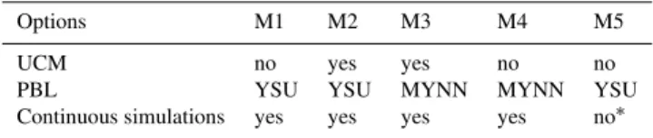
Table 1.Numerical options and physical parameterizations consid-ered.
Options M1 M2 M3 M4 M5
UCM no yes yes no no
PBL YSU YSU MYNN MYNN YSU Continuous simulations yes yes yes yes no∗
∗Restarted every two days.
traffic count data and surveys in many regions (Waked and Afif, 2012). Temporal profiles were allocated with monthly, daily, and diurnal resolutions for all sources. The inventory was developed for a base year of 2010.
3 Meteorological simulations
3.1 Model simulation configurations
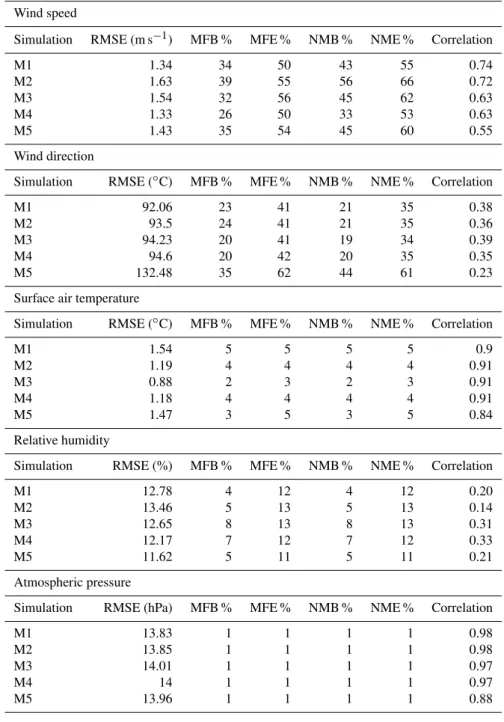
The results obtained from WRF were evaluated with meteo-rological data collected at the USJ site. Reliable meteorolog-ical data at other locations were not available within the D1 and D2 domains, thereby preventing a more complete model performance evaluation. Different simulations from M1 to M5 (Table 1) were performed to select the meteorological simulation that has the lowest biases and errors when com-pared to observations.
For physical parameterizations, the YSU PBL scheme (simulation M2) and the MYNN scheme (simulation M3) were tested with the use of UCM. In addition, two simu-lations (M1 and M4) with the YSU and MYNN schemes, respectively, were performed without the use of UCM. To test numerical options, a simulation (M5) was performed us-ing segmented simulations with two-day restarts to assess whether the model tends to diverge significantly after two days of simulation.
3.2 Results
Table 2.Statistical performance evaluation of the meteorological variables for the WRF simulations.
Wind speed
Simulation RMSE (m s−1) MFB % MFE % NMB % NME % Correlation
M1 1.34 34 50 43 55 0.74
M2 1.63 39 55 56 66 0.72
M3 1.54 32 56 45 62 0.63
M4 1.33 26 50 33 53 0.63
M5 1.43 35 54 45 60 0.55
Wind direction
Simulation RMSE (◦C) MFB % MFE % NMB % NME % Correlation
M1 92.06 23 41 21 35 0.38
M2 93.5 24 41 21 35 0.36
M3 94.23 20 41 19 34 0.39
M4 94.6 20 42 20 35 0.35
M5 132.48 35 62 44 61 0.23
Surface air temperature
Simulation RMSE (◦C) MFB % MFE % NMB % NME % Correlation
M1 1.54 5 5 5 5 0.9
M2 1.19 4 4 4 4 0.91
M3 0.88 2 3 2 3 0.91
M4 1.18 4 4 4 4 0.91
M5 1.47 3 5 3 5 0.84
Relative humidity
Simulation RMSE (%) MFB % MFE % NMB % NME % Correlation
M1 12.78 4 12 4 12 0.20
M2 13.46 5 13 5 13 0.14
M3 12.65 8 13 8 13 0.31
M4 12.17 7 12 7 12 0.33
M5 11.62 5 11 5 11 0.21
Atmospheric pressure
Simulation RMSE (hPa) MFB % MFE % NMB % NME % Correlation
M1 13.83 1 1 1 1 0.98
M2 13.85 1 1 1 1 0.98
M3 14.01 1 1 1 1 0.97
M4 14 1 1 1 1 0.97
M5 13.96 1 1 1 1 0.88
60 %. For surface temperature, relative humidity, and pres-sure, the statistical biases indicate a low overprediction of 1 to 10 %. Accordingly, RMSE reported values for surface temperature (1.54◦C) and wind speed (1.34 m s−1) are low, those of relative humidity (13 %) and pressure (14 hPa) are moderate, and that of wind direction is high (92◦, simulation M1). Thus, model predictions of wind direction are the worst among the five variables. Other studies have shown RMSE values for surface temperature of 2.8◦C in Alaska (Molders, 2008), 3.46◦C in the southern US (Zhang et al., 2006), and 2.82◦C in Paris (Kim, 2011). For wind speed, these values
3.3 Numerical options
The evaluation of segmented simulations is reported in this section because grid nudging of the NCEP initial and bound-ary conditions was used in all simulations. Comparison be-tween simulation M5 (segmented simulations with two-day restarts) and the other simulations (M1–M4) showed bet-ter correlations for all the variables for the long simula-tions without segmentation, especially for wind components where M5 gives correlations of 0.55 and 0.23 for wind speed and wind direction, respectively, compared to values of 0.74 and 0.38 obtained from a long simulation without segmen-tation such as M1. For other variables, differences between simulations are not significant. RMSE and other statistical indicator values are comparable between M5 and the con-tinuous simulations. This leads to the conclusion that the model does not diverge significantly after some integration time, which results in part from the small size of the D1 do-main and its two-way nesting to greater dodo-mains. On the other hand, there is considerable uncertainty in the initial conditions, which are generated every two days in the non-continuous simulations because these initial conditions are provided with a spatial grid spacing of 100 km to be used in a simulation for Beirut with a grid spacing resolution of 1 km, thereby leading to biases and errors that are higher than those of a continuous simulation.
3.4 Physical parameterizations
The MYNN PBL scheme used with UCM (simulation M3) was found to produce the best statistical results for all the variables. Accordingly, this physical option influences wind speed, surface temperature, relative humidity, and pressure. Using this option leads to the best correlations among all the simulations for all variables except for wind speed. The cor-relations are 0.63, 0.39, 0.91, 0.31, and 0.97 for wind speed, wind direction, surface temperature, relative humidity, and pressure. For MFB, MFE, NMB and NME, no significant differences are observed among these simulations (M1-M4). In summary, M1 with the YSU scheme gives the best results for wind speed and M3 with the MYNN scheme and UCM gives the best results for wind direction and relative humid-ity.
3.5 Best configuration
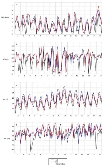
Temporal variations for wind speed, wind direction, surface temperature, and relative humidity of the two best selected simulations (M1 and M3) are shown from 2 July, 00:00 LT to 17 July, 00:00, 2011 in Fig. 2 because no observations were recorded after 17 July 00:00. The model reproduces wind di-rection better from 6 July to 10 July in both simulations while from 2 July to 6 July and from 12 to 16 July, the model is not able to reproduce winds originating from the East. The model reproduces satisfactorily relative humidity for the
se-Fig. 2.Temporal variation of meteorological variables (observations and model simulations M1 and M3) from 2 to 17 July 2011;(a)
wind speed (m s−1);(b)wind direction (◦);(c)air temperature (◦C);
(d)relative humidity (%)).
lected period in simulations except on 4, 5, 15 and 16 July when the model overpredicts relative humidity. Surface tem-perature is better reproduced in simulation M3 than in sim-ulation M1, which overpredicts surface temperature. Lastly, a comparable pattern is observed with lower values for wind speed in simulation M3 due to the use of UCM, which has an effect of decreasing wind speeds due to urbanization. In summary, the model performs better from 6 to 10 July for all the variables.
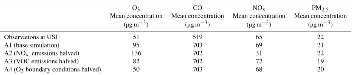
Table 3.Results from simulations A1 to A4 from 2 to 18 July 2011 at USJ.
O3 CO NOx PM2.5
Mean concentration Mean concentration Mean concentration Mean concentration (µg m−3) (µg m−3) (µg m−3) (µg m−3)
Observations at USJ 51 519 65 22
A1 (base simulation) 95 703 69 21
A2 (NOx emissions halved) 136 702 31 22
A3 (VOC emissions halved) 82 702 72 19
A4 (O3boundary conditions halved) 50 703 68 20
speed and wind direction, no significant variation is observed between M1 and M3. For relative humidity, a better correla-tion is obtained using the MYNN PBL scheme, and a lower non-significant correlation is obtained for wind speed. Over-all, simulation M3 performs slightly better for most variables than simulation M1 particularly for temperature and humid-ity and we may consider that the correlation of 0.63 obtained for wind speed in simulation M3 is close to the correlation of 0.74 (systematic error of 18 %) obtained in simulation M1 while the correlation for relative humidity of 0.31 obtained in simulation M3 is significantly different from the value of 0.2 (systematic error of 43 %) obtained in simulation M1. In addition, surface air temperature and wind direction were slightly better modeled in simulation M3 in terms of tem-poral variation (Fig. 2) and NMB (Table 2). Based on these considerations, the results obtained from simulation M3 are used for air quality modeling.
4 Air quality simulations
The results obtained from Polyphemus/Polair3D were eval-uated against measurements of gaseous species (O3, NO2, VOC and CO) and PM2.5 (total mass and major compo-nents) collected at the USJ site. Statistical indicators used for model evaluation include MFB, MFE, mean normalized bias (MNB), and mean normalized error (MNE) (e.g., Yu et al., 2006).
4.1 Gaseous species
The base simulation conducted with the MOZART-4 bound-ary conditions (Simulation A1) led to O3 concentrations within the D1 domain that were too high compared to the ob-servations by nearly a factor of two (see Table 3). Sensitivity simulations were conducted where emissions of NOx (Simu-lation A2) and VOC (Simu(Simu-lation A3) were reduced by a fac-tor of two; these simulations did not lead to satisfacfac-tory O3 concentrations, in part because of the strong influence of the boundary conditions. A decrease of NOxemissions leads to an increase in O3concentrations (A2) because the study area is saturated in NOx. Moreover, NOxconcentrations are well reproduced by the model in the base simulation A1. VOC
reductions are effective in reducing O3concentrations (A3) due to the fact that the area of the study is considered to be VOC-limited, having a VOC to NOxratio in the range of 3 to 5. However, the decrease in O3concentrations is insufficient to match the observed concentrations and VOC concentra-tions are already underestimated by the model in A1 by a factor of 2 to 3 (Table 4). An increase of NOxemissions and a decrease of VOC emissions could lead to satisfactory O3 concentrations, but would lead to non-satisfactory results for VOC and NOxmodeled concentrations. Therefore, a sensi-tivity simulation was also conducted with the boundary O3 concentrations halved (Simulation A4). That simulation led to reasonable agreement with the observations for all gaseous species. A comparison between simulation A1 and simula-tion A4 shows that modifying the O3boundary concentra-tions has negligible effect on CO, NOxand PM2.5modeled concentrations. Although a recent evaluation of MOZART-4 with ozone study led to satisfactory results (Emmons et al., 2010), a detailed evaluation with PBL O3data in the Mid-dle East region has not been conducted because of a lack of data. Better characterization of PBL air pollution concentra-tions in that region is needed to obtain realistic O3boundary concentrations.
This strong influence of boundary conditions, which leads to a significant overestimation of O3concentrations, may be due to the fact that the MOZART-4 data used during this study have a horizontal resolution of 280 km and are used as boundary conditions for a domain D2 with a horizontal res-olution of 5 km. It is possible that the use of an intermediate domain of 25 or 50 km horizontal resolution may decrease the uncertainties generated by the MOZART-4 data. How-ever, an emission inventory for the Middle East region is not currently available and the use of an intermediate domain D3 for air quality simulation is, therefore, not feasible.
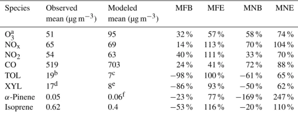
Table 4.Statistical performance evaluation for O3, NO2, NOx, CO and some VOC at USJ for the simulation A1.
Species Observed Modeled MFB MFE MNB MNE mean (µg m−3) mean (µg m−3)
Oa3 51 95 32 % 57 % 58 % 74 % NOx 65 69 14 % 113 % 70 % 104 %
NO2 54 63 40 % 111 % 33 % 70 % CO 519 703 24 % 41 % 72 % 88 % TOL 19b 7c −98 % 100 % −61 % 65 % XYL 17d 8e −86 % 93 % −50 % 62 %
α-Pinene 0.05 0.06f −23 % 77 % −169 % 247 % Isoprene 0.62 0.4 −53 % 116 % −20 % 110 %
aA threshold value of 80 µg m−3was used for observations.
bThe “TOL” measured species include toluene, ethylbenzene, butylbenzene, isopropylbenzene and propylbenzene. cThe “TOL” modeled species includes also other minor monosubstituted aromatics.
dThe “XYL” measured species includes xylene, trimethylbenzenze and ethyltoluene. eThe “XYL” modeled species includes also other minor polysubstituted aromatics. fThe “α-pinene” modeled species includesα-pinene and sabinene.
possible biases in the air quality simulation if the differ-ences cannot be justified. The results show a modeled value of 1585 µg m−3for CO in both simulations A1 and A4 com-pared to a measured value of 1213 µg m−3. For PM10, a value of 47 µg m−3was modeled in both simulations compared to a measured value of 44 µg m−3. The modeled O
3 concen-trations are 54 µg m−3 in simulation A1 and 32 µg m−3 in simulation A4, compared to a measured value of 34 µg m−3. Clearly, the results obtained from this evaluation show that simulation A4 with modified O3boundary conditions leads to better results for O3concentrations and has negligible ef-fect on other pollutants. The results obtained from simula-tions A1 and A4 are presented and evaluated against mea-surements below.
Average modeled surface concentrations (over both land and sea) of O3, NO2, and CO from 2 to 18 July are 50, 49 and 700 µg m−3 in the inner domain (D1) and 72, 10 and 240 µg m−3in the outer domain (D2), respectively, in sim-ulation A4. In simsim-ulation A1, average modeled surface con-centrations for O3were 125 and 103 µg m−3for the domains D2 and D1, respectively. For other gaseous pollutants such as NO2 (58 µg m−3 for D2 and 10 µg m−3 for D1) and CO (768 µg m−3for D2 and 245 µg m−3for D1), modeled con-centrations were comparable between simulations A1 and A4.
The modeled values for O3and NO2in the inner domain (simulation A4) are comparable to the average annual mod-eled values of 47 µg m−3 and 52 µg m−3 for O3 and NO2, respectively, obtained in a modeling study over the Iberian Peninsula in the northwestern Mediterranean region for a base year of 2004 using a coupled WRF/CMAQ model (Ji-men´ez-Guerrero et al., 2008).
The modeled surface spatial distributions of O3and NO2 concentrations for D2 and D1 (Figs. 3 and 4) show lower O3concentrations where most NOx emissions from indus-tries, harbors and road traffic occur and higher values in the
mountains. Accordingly, higher concentrations of NO2 are modeled near the coast in Beirut and its suburbs, in the cities of Tripoli and Chekka in the north and Jieh in the south. Ma-jor sources in those areas include dense traffic in urban areas and on highways along the coast, in particular in Beirut and Tripoli, the Zouk power plant located on the coast north of Beirut, the Jieh power plant and the cement plants located in the city of Chekka. Other emissions are generated from the harbors in Beirut and Tripoli and from the international airport located on the coast south of Beirut. Higher O3 con-centrations modeled in the mountains (east of the domain) might be related to a higher VOC/NOx ratio (Fig. 5), which is more favorable to O3formation.
To evaluate the model concentration results at the USJ site, different statistical metrics were calculated for the 2–18 July period, as shown in Table 4 for the simulation A1 and in Ta-ble 5 for the simulation A4.
1
D D T
C
B
J
a b
c d
Fig. 3.Modeled average O3concentrations ((a)simulation A1 and
(b)simulation A4) and NO2concentrations ((c)simulation A1 and
(d)simulation A4) in µg m−3for the outer domain D2 (T=Tripoli; C=Chekka; B=Beirut; J=Jieh).
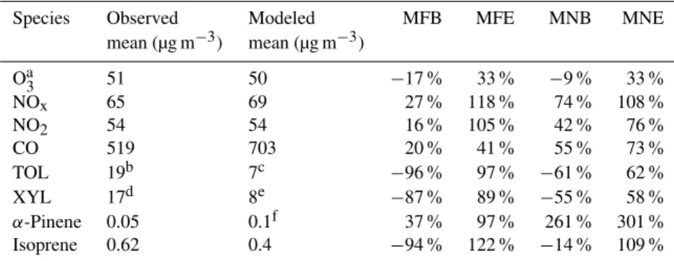
a modeling study at the Iberian Peninsula over the Mediter-ranean basin with the use of a different CTM model (Ji-men´ez-Guerrero et al., 2008). However, the value of 40 % obtained in simulation A1 is greater by nearly a factor of two, because of the O3overestimation. However, MNB values of 74 % (simulation A4) and 70 % (simulation A1) for NOx cal-culated during this study are in better agreement with ob-servations than the reported value of 101 % for a simulation over Nashville, USA, in July 1999 using the CMAQ model (Bailey et al., 2007). CO concentrations show an overpredic-tion by the model on the order of 30 % on average. These results are comparable to those of other studies conducted in Europe, Mexico and the USA (Matthias et al., 2008; Zhang et al., 2009; Bailey et al., 2007). In contrast, CO modeled average concentrations in Spain were underpredicted by the model with an MFB value of−26 % (Jimen´ez-Guerrero et al., 2008) with the same order of magnitude as those calcu-lated MFB for Beirut (20 % and 24 %; Tables 4 and 5).
Biogenic VOC concentrations are small (<1 µg m−3)for both observations and simulations; they show an overpredic-tion ofα-pinene by the model by a factor of two in simulation A4 and a good agreement between modeled and measured values in simulation A1 due to the fact that VOC such as α-pinene may be consumed in the simulation A1 to form O3 because the inner domain D2 is VOC limited. For isoprene, an underprediction on the order of 30 % was calculated. The overprediction ofα-pinene in simulation A4 could be related to the fact thatα-pinene model species is a surrogate species that includes α-pinene and sabinene. The MNB values of −20 and−14 % (Tables 4 and 5) reported for isoprene are
1
a b
c d
Fig. 4.Modeled average O3concentrations ((a)simulation A1 and
(b)simulation A4) and NO2concentrations ((c)simulation A1 and
(d)simulation A4) in µg m−3for the inner domain D2. The red dot corresponds to the location of the measurement site at USJ during July 2011.
Fig. 5.Modeled average VOC/NOxratio for the inner domain D1.
Table 5.Statistical performance evaluation for O3, NO2, NOx, CO and some VOC at USJ for the simulation A4.
Species Observed Modeled MFB MFE MNB MNE mean (µg m−3) mean (µg m−3)
Oa3 51 50 −17 % 33 % −9 % 33 % NOx 65 69 27 % 118 % 74 % 108 %
NO2 54 54 16 % 105 % 42 % 76 % CO 519 703 20 % 41 % 55 % 73 % TOL 19b 7c −96 % 97 % −61 % 62 % XYL 17d 8e −87 % 89 % −55 % 58 %
α-Pinene 0.05 0.1f 37 % 97 % 261 % 301 % Isoprene 0.62 0.4 −94 % 122 % −14 % 109 %
aA threshold value of 80 µg m−3was used for observations.
bThe “TOL” measured species include toluene, ethylbenzene, butylbenzene, isopropylbenzene and propylbenzene. cThe “TOL” modeled species includes also other minor monosubstituted aromatics.
dThe “XYL” measured species includes xylene, trimethylbenzenze and ethyltoluene. eThe “XYL” modeled species includes also other minor polysubstituted aromatics. fThe “α-pinene” modeled species includesα-pinene and sabinene.
Table 6.Statistical performance evaluation for PM2.5, OC, EC and particulate sulfate, nitrate and ammonium at USJ for the simulation A1.
Species Observed Modeled RMSE MFB MFE mean (µg m−3) mean (µg m−3) (µg m−3)
PM2.5 21.9 21.32 9.75 −19% 38 %
OC 5.6 3.31 3.32 −62 % 65 %
EC 1.8 1.22 1.06 −33 % 56 %
Sulfate 6.06 8.10 5.35 26 % 61 % Nitrate 0.32 0.008 0.39 −186 % 186 % Ammonium 1.87 0.32 1.9 −113% 128%
Date
O
3
µg.m
-3
0 50 100 150 200
Observations A4
A1
2 3 4 5 6 7 8 9 10 11 12 13 14
Fig. 6.Temporal variation of observed and modeled O3 concentra-tions in µg m−3from 2 to 13 July 2011.
monoterpene concentrations are underestimated by almost a factor of two in a simulation over the eastern US using the MOZART-4 CTM (Horowitz et al., 2007) due to a significant underestimation in terpene emissions while isoprene emis-sion estimates can differ by more than a factor of 3 for spe-cific times and locations when different driving variables are used in the emissions calculations (Guenther et al., 2006).
1
T
C
B
J
a b
c d
Fig. 7. Modeled average PM2.5 concentrations in µg m−3 in
Table 7.Statistical performance evaluation for PM2.5, OC, EC and particulate sulfate, nitrate and ammonium at USJ for the simulation A4.
Species Observed Modeled RMSE MFB MFE mean (µg m−3) mean (µg m−3) (µg m−3)
PM2.5 21.9 19.93 9.89 −21 % 39 %
OC 5.6 3.24 2.93 −59 % 61 %
EC 1.8 1.17 1.05 −33 % 56 %
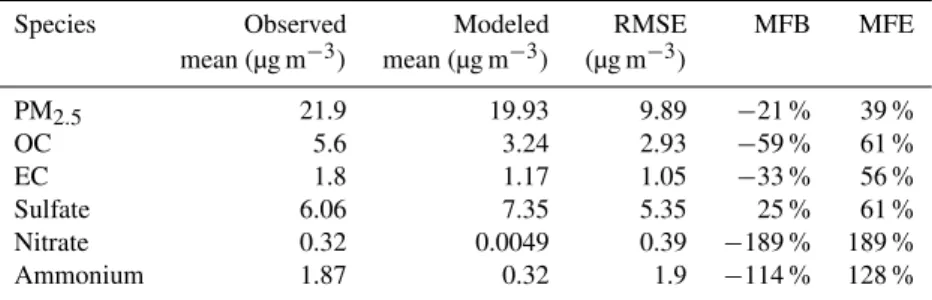
Sulfate 6.06 7.35 5.35 25 % 61 % Nitrate 0.32 0.0049 0.39 −189 % 189 % Ammonium 1.87 0.32 1.9 −114 % 128 %
Temporal variations for O3are shown in Fig. 6 from 2 to 13 July 2011 (no measurements were recorded after 13 July). The model reproduces satisfactorily the diurnal variation of O3, with a peak O3concentration occurring between 12 p.m. and 1 p.m. for both observed and modeled values on most days. This day peak is typical for O3 and was observed in many modeling studies of air pollution and measurements and is related to the formation of O3 during the day from precursors such as NOx, CO and VOC in the presence of in-tense solar radiation. However, on some days (3, 5, and 8 July), a second nonsignificant O3peak is observed between 9 a.m. and 10 a.m. This second peak is not reproduced by the model. The observed peak could be related in part to variabil-ity in the measured O3concentrations (fluctuations) during a wide peak period. This second peak could also be related to the road traffic diurnal variations when vehicle emissions decrease slowly during the day time peak between 10 a.m. and 11 a.m. (Waked and Afif, 2012; Waked et al., 2012) and, therefore, account for a decrease in O3formation. Although the diurnal variations of road traffic are included in this mod-eling study, the tendency of the model to normalize these fluctuations during the O3 peak and the uncertainties asso-ciated with wind directions on some days could contribute to the discrepancy between the observations and the model.
4.2 Particulate pollutants
Modeled PM2.5 average surface concentrations (over both land and sea) from 2 to 18 July 2011 are 10 µg m−3 (sim-ulations A1 and A4) for Lebanon (D2) and 21 and 19 µg m−3 (simulations A1 and A4) for Beirut and its suburbs (D1). The spatial distribution of PM2.5concentrations (Fig. 7) shows higher concentrations (>40 µg m−3) in the city of Beirut and its northern suburb, Chekka in the north and Sibline in the south. Dense on-road traffic, industrial sources (Zouk plant north of Beirut and the cement plants near the coast of Chekka and Sibline) and Beirut international airport lo-cated south of Beirut lead to significant air pollutant emis-sions (Waked et al., 2012). Lower PM2.5 concentrations in the eastern part of the domains (<20 µg m−3), are related to the fact that anthropogenic sources in these areas are less significant. This suggests that PM2.5concentrations are dom-inated by anthropogenic sources. Indeed, biogenic modeled
SOA account for only 4 % of total PM2.5 modeled concen-trations in the inner domain D1 and 8 % in the outer domain D2. Compared to the WHO annual guideline of 10 µg m−3 and 24 h average guideline of 25 µg m−3, PM2.5 concentra-tions exceed these values in large urban agglomeraconcentra-tions such as Beirut and Tripoli and in the regions of Chekka and Sibline where several cement plants are located and modeled PM2.5 are above 100 µg m−3.
Statistical model performance at the USJ site are presented in Tables 6 and 7. The observed value for PM2.5is a recon-structed mass concentration based on the IMPROVE method (IMPROVE, 2011; PM2.5=1.8·OC+EC+1.375·sulfate +1.29·nitrate+1.8·Cl+2.2·Al+2.49·Si+1.63·Ca +2.42·Fe+1.94·Ti). Overall, the model reproduces sat-isfactorily PM2.5, OC, EC, and sulfate (SO24−)average con-centrations. MFB values in the range of−62 to 25 % and MFE values in the range of 39 to 65 % obtained during this study indicate that the model meets the performance criteria (−60 %≤MFB≤ +60 % and MFE ≤75 %) proposed by Boylan and Russel (2006). For nitrate and ammonium, there is a large underestimation of the model. This high underesti-mation could be related in part to uncertainties in NH3 emis-sions. On the other hand, the measured nitrate concentrations could be overestimated due to adsorption of nitric acid on the particulate filters because no denuder was placed upstream of the filters. The MFB and MFE reported values of−59 and −62 % and 61 and 65 % obtained for OC during this study are in agreement with the values of−37 % and 50 % reported for Europe in another simulation conducted using Polyphe-mus/Polair3D (Couvidat et al., 2012). In a simulation con-ducted with the CMAQ model over the eastern US, MFB values for PM2.5, OC and EC were −3 %, 37 % and 14 %, respectively (Bailey et al., 2007). Those are lower than the values reported here (Tables 6 and 7). However, for sulfate a MFB of 25–26 % reported here is lower in absolute value than the value of−35 % reported by Bailey et al. (2007).
5 Conclusion and future prospects
the diurnal variations for temperature, wind speed, relative humidity and atmospheric pressure and agrees relatively well with observation of wind direction especially from 6 to 10 July 2011. The WRF results show acceptable performance compared to other studies in Europe and the United States; however, measurements were available for model perfor-mance evaluation only at one site. The air quality model-ing results in Beirut, show higher NO2concentrations near the coast in the city of Beirut and its northern suburb and lower O3concentrations within the city limits. Highest val-ues for PM2.5, OC, and EC are modeled within the city lim-its suggesting that the major sources that lead to the forma-tion of PM2.5are anthropogenic sources. The CTM perfor-mance evaluation results show that Polyphemus/Polair3D re-produces satisfactorily O3(simulation A4), PM2.5, OC, EC, and sulfate concentrations (both simulations A1 and A4).
Statistical indicators obtained for the major pollutants are in the range of other studies conducted in Europe and US, Furthermore, the O3diurnal variation is well reproduced by the model, except for secondary morning peaks that are ob-served on some days but not reproduced by the model. This modeling study is the first one conducted for Beirut. It pro-vides an overview of the pollutant concentrations in the sum-mer of 2011. Future work should focus on the improve-ment of the input data such as the emission inventory and the meteorology in order to reduce bias and errors between modeled and observed concentrations. Accordingly, specific emission factors for Lebanon, which are inexistent up to now, are needed as future improvements. These emissions factors could be obtained through measurement campaigns at sev-eral point sources. In particular, a measurement campaign in a road tunnel in Beirut is highly recommended in order to ob-tain specific road transport emission factors representative of the Lebanese fleet. Moreover, the development of a regional emission inventory for the Middle East region would help to reduce biases and errors generated from the boundary con-ditions due to large uncertainties related to emission inven-tories in this region. Furthermore, observational data from more than one site, typically two or three sites in the city of Beirut, are needed to better evaluate the model. In particu-lar, measurements of meteorological variables at many sites are needed to better reproduce the meteorology through data assimilation and measurements of particulate pollutants and gases are needed to evaluate the model accuracy to repro-duce these pollutant concentrations in various areas of the study domain. In addition, measurements of meteorology and pollutant concentrations aloft, including the PBL height are needed in order to evaluate the ability of the meteorological and air quality models to reproduce the complex processes of land-sea breeze, mountain valley winds, and the urban heat island.
Acknowledgements. Funding for this study was provided by ´
Ecole des Ponts ParisTech, the Lebanese National Council for Scientific Research and the Saint Joseph University (Faculty of Sciences and the Council for Research). The authors acknowledge Thierry Leonardis, Servanne Chevaillier and Sylvain Triquet for providing observational data for CO, VOC, NOx, O3 and major
components of fine particulate matter (PM2.5).
Edited by: Y. Balkanski
References
Afif, C., Dutot, A., Jambert, C., Abboud, M., Adjizian-G´erard, J., Farah, W., Perros, P., and Rizk, T.: Statistical approach for the characterization of NO2 concentrations in Beirut, Air Quality,
Atmosphere & Health, 2, 57–67, 2009.
Borge, R., Alexandrov, V., Jos´e del Vas, J., Lumbreras, J., and Ro-driguez, E.: A comprehensive sensitivity analysis of the WRF model for air quality applications over the Iberian Peninsula, At-mos. Environ., 42, 8560–8574, 2008.
Bailey, E. M., Gautney, L. L., Kelsoe, J. J., Jacobs, M. E., Mao, Q., Condrey, J. W., Pun, B., Yu, S. Y., Seigneur, C., Dou-glas, S., Heney, J., and Kumar, N.: A comparison of the per-formance of four air quality models for the Southern oxidants study episode in July 1999, J. Geophys. Res., 112, D05306, doi:10.1029/2005JD007021, 2007.
Boylan, J. W. and Russell, A. G.: PM and light extinction model performance metrics, goals, and criteria for three-dimensional air quality models, Atmos. Environ., 40, 4946–4959, 2006. Byun, D. and Schere, K. L.: Review of the governing equations,
computational algorithms and other components of the models-3 community multi scale air quality (CMAQ) modeling system, Applied Mechanics Review, 59, 51, 2006.
Carvalho, D., Rocha, A., Gomez-Gesteira, M., and Santos, C.: A sensitivity study of WRF model in wind simulation for an area of high wind energy, Environ. Modell. Softw., 33, 23–34, 2012. Cavalli, F., Viana, M., Yttri, K. E., Genberg, J., and Putaud, J.-P.:
Toward a standardised thermal-optical protocol for measuring atmospheric organic and elemental carbon: the EUSAAR proto-col, Atmos. Meas. Tech., 3, 79–89, doi:10.5194/amt-3-79-2010, 2010.
CBDE, Consensus of buildings and establishments report. Cen-tral Administrate of Statistics, Beirut, Lebanon, www.cas.gov.lb, 2004.
Ch´elala, C.: Transport routier et pollution de l’air en NO2, PhD
the-sis, Universit´e Saint Joseph, Lebanon, 2008.
Chen, W., Kuze, H., Uchiyama, A., Suzuki, Y., and Takeuchi, N.: One-year observation of urban mixed layer characteristics at Tsukuba, Japan using a micro pulse lidar, Atmos. Environ., 35, 4273–4280, 2001.
Chou, M.-D. and Suarez, M. J.: An efficient thermal infrared ra-diation parameterization for use in general circulation models, NASA Technical Memorandum, 104606, 3:85, 1994.
Couvidat, F., Debry, ´E., Sartelet, K., and Seigneur, C.: A hy-drophilic/hydrophobic organic (H2O) aerosol model: Develop-ment, evaluation and sensitivity analysis, J. Geophys. Res., 117, D10304, doi:10.1029/2011JD017214, 2012.
application to Paris, France, Atmos. Chem. Phys., 13, 983–996, doi:10.5194/acp-13-983-2013, 2013.
Debry, E., Fahey, K., Sartelet, K., Sportisse, B., and Tombette, M.: Technical Note: A new SIze REsolved Aerosol Model (SIREAM), Atmos. Chem. Phys., 7, 1537–1547, doi:10.5194/acp-7-1537-2007, 2007.
Emmons, L. K., Walters, S., Hess, P. G., Lamarque, J.-F., Pfister, G. G., Fillmore, D., Granier, C., Guenther, A., Kinnison, D., Laepple, T., Orlando, J., Tie, X., Tyndall, G., Wiedinmyer, C., Baughcum, S. L., and Kloster, S.: Description and evaluation of the Model for Ozone and Related chemical Tracers, version 4 (MOZART-4), Geosci. Model Dev., 3, 43–67, doi:10.5194/gmd-3-43-2010, 2010.
ESCWA. Transport for sustainable development for the Arab re-gion: Measures, progress achieved, Challenge and policy frame-work report, http://www.escwa.un.org/information/publications/ edit/.../SDPD-09-w1.pdf, 2010.
Gilliam, R. C., Hogrefe, C., and Rao, S.: New methods for evalu-ating meteorological models used in air quality applications, At-mos. Environ., 40, 5073–5086, 2006.
Grell, G. A. and Devenyi, D.: A generalized approach to param-eterizing convection combining ensemble and data assimilation techniques, Geophys. Res. Lett., 29, 38.1–38.4, 2002.
Grell, G. A., Peckham, S. E., Schmitz, R., McKeen, S. A., Frost, G., Skamarock, W. C., and Eder, B.: Fully coupled online chemistry within the WRF model, Atmos. Environ., 39, 695–6975, 2005. Guenther, A., Karl, T., Harley, P., Wiedinmyer, C., Palmer, P. I.,
and Geron, C.: Estimates of global terrestrial isoprene emissions using MEGAN (Model of Emissions of Gases and Aerosols from Nature), Atmos. Chem. Phys., 6, 3181–3210, doi:10.5194/acp-6-3181-2006, 2006.
Hong, S.-Y., Noh, Y., and Dudhia, J.: A new vertical diffusion pack-age with an explicit treatment of entrainment processes, Mon. Weather Rev., 134, 2318–2341, 2006.
Horowitz, L. W., Fiore, A. M., Milly, G. P., Cohen, R. C., Perring, A., Wooldridge, P. J., Hess, P. G., Emmons, L. K., and Lamar-que, J. F.: Observational constraints on the chemistry of isoprene nitrates over the eastern United States, J. Geophys. Res., 112, D12S08, doi:10.1029/2006JD007747, 2007.
IIASA: Average annual anthropogenic heat flux for major cap-ital cities in the world, Retrieved from http//www.iiasa.ac.at/ research/TNT/WEB/heat/, 2012.
IMPROVE: Spatial and seasonal patterns and temporal variability of haze and its constituents in the United States: Report V, June, 2011. Interagency monitering of protected visual environement, chapter 2,Spatial patterns of speciated PM2.5aerosol mass
con-centrations, 38 pp., available at: http://vista.cira.colostate.edu/ improve/publications/Reports/2011/PDF/Chapter2.pdf, 2011. Jim´enez-Guerrero, P., Jorba, O., Baldasano, J. M., and
Gasso, S.: The use of a modelling system as a tool for air quality management: Annual high-resolution simula-tions and evaluation, Sci. Total Environ., 390, 323–340, doi:10.1016/j.scitotenv.2007.10.025, 2008.
Kessler, E.: On the distribution and continuity of water substance in atmospheric circulation, Meteorological Monographs, 32, 84 pp., 1969.
Kim, Y.: Mod´elisation de la qualit´e de l’air: ´Evaluation des param´etrisations chimiques et m´et´eorologiques, PhD thesis, 159 pp., 2011.
Kim, Y., Sartelet, K., and Seigneur, C.: Comparison of two gas-phase chemical kinetic mechanisms of ozone formation over Eu-rope, J. Atmos. Chem., 62, 89–119, 2009.
Kim, Y., Couvidat, F., Sartelet, K., and Seigneur, C.: Comparison of different gas-phase mechanisms and aerosol modules for simu-lating particulate matter formation, J. Air Waste Manage. Assoc., 61, 126, 2011.
Kouvarakis, G., Tsigaridis, K., Kanakidou, M., and Mihalopoulos, N.: Temporal variations of surface regional background ozone over Crete Island in the southeast Mediterranean, J. Geophys. Res., 105, 4399–4407, 2000.
Kusaka, H., Kondo, H., Kikegawa, Y., and Kimura, F.: A Simple Single-Layer Urban Canopy Model For Atmospheric Models: Comparison With Multi-Layer And Slab Models, Bound.-Lay. Meteorol., 101, 329–358, 2001.
Lelieveld, J., Berresheim, H., Borrmann, S., Crutzen, P. J., Den-tener, F. J., Fischer, H., Feichter, J., Flatau, P. J., Heland, J., Holzinger, R., Korrmann, R., Lawrence, M. G., Levin, Z., Markowicz, K. M., Mihalopoulos, N., Minikin, A., Ramanathan, V., de Reus, M., Roelofs, G. J., Scheeren, H. A., Sciare, J., Schlager, H., Schultz, M., Siegmund, P., Steil, B., Stephanou, E. G., Stier, P., Traub, M., Warneke, C., Williams, J., and Ziereis, H.: Global Air Pollution Crossroads over the Mediterranean, Sci-ence, 298, 794–799, 2002.
Lelieveld, J., Hoor, P., J¨ockel, P., Pozzer, A., Hadjinicolaou, P., Cammas, J.-P., and Beirle, S.: Severe ozone air pollution in the Persian Gulf region, Atmos. Chem. Phys., 9, 1393–1406, doi:10.5194/acp-9-1393-2009, 2009.
Liu, J., Jones, D., Worden, J., Noone, D., Parrington, M., and Kar, J.: Analysis of the summertime buildup of tropospheric ozone abun-dances over the Middle East and North Africa 15 as observed by the Tropospheric Emission Spectrometer instrument, J. Geophys. Res., 114, D05304, doi:10.1029/2008JD010993,6345, 2009. Louis, J.-F.: A parametric model of vertical eddy fluxes in the
atmo-sphere. Bound.-Lay. Meteorol., 17, 187–202, 1979.
Mallet, V., Qu´elo, D., Sportisse, B., Ahmed de Biasi, M., Debry, ´
E., Korsakissok, I., Wu, L., Roustan, Y., Sartelet, K., Tombette, M., and Foudhil, H.: Technical Note: The air quality model-ing system Polyphemus, Atmos. Chem. Phys., 7, 5479–5487, doi:10.5194/acp-7-5479-2007, 2007.
Martilli, A., Clappier, A., and Rotach, M. W.: An Urban Surface Exchange Parameterisation for Mesoscale Models, Bound.-Lay. Meteorol., 104, 261–304, 2002.
Massoud, R., Shihadeh, A., Roumi´e, M., Youness, M., Gerard, J., Saliba, N., Zaarour, R., Abboud, M., Farah, W., and Saliba, N. A.: Intraurban variability of PM10 and PM2.5in an Eastern
Mediter-ranean city, Atmos. Res., 101, 893–901, 2011.
Matthias, V., Aulinger, A., and Quante, M.: Adapting CMAQ to in-vestigate air pollution in north Sea coastal region, Environ. Mod-ell. Softw., 23, 356–368, 2008.
Mlawer, E. J., Taubman, S. J., Brown, P. D., Iacono, M. J., and Clough, S. A.: Radiative transfer for inhomogeneous atmo-spheres : RRTM, a validated correlated-k model for thelongwave, J. Geophys. Res., 102, 16663–16682, 1997.
Mellor, G. L and Yamada, T.: A hierarchy of turbulence closure models for planetary boundary layers, J. Atmos. Sci., 31, 1791– 1806, 1974.
Molders, N.: Suitability of the Weather Research and Forecasting (WRF) Model to Predict the June 2005 Fire Weather for Interior Alaska, Weather Forecast., 23, 953–973, 2008.
Nakanishi, M. and Niino, H.: An Improved Mellor – Yamada Level-3 Model with Condensation Physics: Its Design and Verification, Bound.-Lay. Meteorol., 112, 1–31, 2004.
Nenes, A., Pandis, S. N., and Pilinis, C.: ISORROPIA : A new ther-modynamic equilibrium model for multiphase multicomponent inorganic aerosols, Aquat. Geochem., 4, 123–152, 1998. Roeckner, E., Brokopf, R., Esch, M., Giorgetta, M., Hagemann, S.,
Kornbluh, L., Manzini, L. E., Schlese, U., and Schulzweida, U.: Sensitivity of simulated climate to horizontal and vertical reso-lution in the ECHAM5 atmosphere model, J. Climate, 19, 3771– 3791, 2006.
Russell, A. and Dennis, R.: NARSTO critical review of photochem-ical models and modeling, Atmos. Environ., 34, 2283–2324, 2000.
Salamanca, F., Krpo, A., Martilli, A., and Clappier, A.: A new build-ing energy model coupled with an urban canopy parameteriza-tion for urban climate simulaparameteriza-tions – part I. formulaparameteriza-tion, verifica-tion, and sensitivity analysis of the model, Theor. Appl. Clima-tol., 99, 331–344, 2010.
Saliba, N. A., Moussa, S., Salame, H., and El-Fadel, M.: Variation of selected air quality indicators over the city of Beirut, Lebanon: Assessment of emission sources, Atmos. Environ., 40, 3263– 3268, 2006.
Saliba, N. A., Kouyoumdjian, H., and Roumi´e, M.: Effect of local and long-range transport emissions on the elemental composition of PM10−2.5and PM2.5in Beirut, Atmos. Environ., 41, 6497–
6509, 2007.
Sartelet, K. N., Debry, E., Fahey, K., Roustan, Y., Tombette, M., and Sportisse, B.: Simulation of aerosols and gas-phase species over Europe with the Polyphemus system: Part I: Model-to-data comparison for 2001, Atmos. Environ., 41, 6116–6131, 2007. Sartelet, K. N., Hayami, H., and Sportisse, B.: MICS Asia Phase II:
”Sensitivity to the aerosol module, Atmos. Environ., 42, 3562– 3570, 2008.
Sartelet, K. N., Couvidat, F., Seigneur, C., and Roustan, Y.: Im-pact of biogenic emissions on air quality over Europe and North America, Atmos. Environ., 53, 131– 141, 2012.
Skamarock, W. C., Klemp, J. B., Dudhia, J., Gill, D. O., Barker, D. M., Duda, M. G., Wang, X.-Y. H. W., and Powers, J. G.: A description of the Advanced Research WRF version 3. NCAR Technical note, -475+STR, 2008.
Smoydzin, L., Fnais, M., and Lelieveld, J.: Ozone pollution over the Arabian Gulf – role of meteorological conditions, Atmos. Chem. Phys. Discuss., 12, 6331–6361, doi:10.5194/acpd-12-6331-2012, 2012.
Stavrakou, T., M¨uller, J. F., Boersma, K. F., De Smedt, I., and van der A, R. J.: Assessing the distribution and growth rates of NOx emission sources by inverting a 10-year record
of NO2 satellite columns, Geophys. Res. Lett., 35, L10801,
doi:10.1029/2008GL033521, 2008.
Stull, R. B.: An introduction to boundary layer meteorology, Kluwer Academic Publishers, Dordrecht, 1988.
Troen, I. B. and Mahrt, L.: A simple model of the atmospheric boundary layer, sensitivity to surface evaporation, Bound.-Lay. Meteorol., 37, 129–148, 1986.
Waked, A.: Caract´erisation des aerosols organiques `a Beyrouth, Liban, PhD thesis, 173 pp., 2012.
Waked, A. and Afif, C. Emissions of air pollutants from road trans-port in Lebanon and other countries in the Middle East region, Atmos. Environ., 61, 446–452, 2012.
Waked, A., Afif, C., and Seigneur, C.: An atmospheric emission inventory of anthropogenic and biogenic sources for Lebanon, Atmos. Environ., 50, 88–96, 2012.
Yarwood, G., Rao, S., Yocke, M., and Whitten, G.: Updates to the carbon bond chemical mechanism: CB05 final report to the US EPA, RT-0400675, 2005.
Yu, S., Eder, B., Dennis, R., Chu, S.-H., and Schwartz, S. E.: New unbiased symmetric metrics for evaluation of air quality models, Atmos. Sci. Lett., 7, 26–34, 2006.
Zhang, Y., Liu, P., Pun, B., and Seigneur, C.: A comprehensive performance evaluation of MM5-CMAQ for the summer 1999 Southern Oxidants Study episode Part I: Evaluation protocols, databases, and meteorological predictions, Atmos. Environ., 40, 4825–4838, 2006.