Annales
Geophysicae
Reconstruction of the ion plasma parameters from the current
measurements: mathematical tool
E. S´eran1
1CETP, Observatoire de Saint-Maur, 4, Avenue de Neptune, 94107 Saint-Maur-des-Foss´es, Cedex, France
Received: 9 April 2002 – Revised: 22 November 2002 – Accepted: 27 November 2002
Abstract. Instrument d’Analyse du Plasma (IAP) is one of the instruments of the newly prepared ionospheric mission Demeter. This analyser was developed to measure flows of thermal ions at the altitude of∼750 km and consists of two parts: (i) retarding potential analyser (APR), which is utilised to measure the energy distribution of the ion plasma along the sensor look direction, and (ii) velocity direction analyser (ADV), which is used to measure the arrival angle of the ion flow with respect to the analyser axis. The necessity to ob-tain quick and precise estimates of the ion plasma parameters has prompted us to revise the existing mathematical tool and to investigate different instrumental limitations, such as (i) finite angular aperture, (ii) grid transparency, (iii) potential depression in the space between the grid wires, (iv) losses of ions during their passage between the entrance diaphragm and the collector. Simple analytical expressions are found to fit the currents, which are measured by the APR and ADV collectors, and show a very good agreement with the numeri-cal solutions. It was proven that the fitting of the current with the model functions gives a possibility to properly resolve even minor ion concentrations and to find the arrival angles of the ion flow in the multi-species plasma. The discussion is illustrated by an analysis of the instrument response in the ionospheric conditions which are predicted by the Interna-tional Reference Ionosphere (IRI) model.
Key words. Ionosphere (plasma convection; instruments and techniques) – Space plasma physics (experimental and mathematical techniques)
1 Introduction
The idea to use retarding and drift analysers for diagnostics of the cold ion population is not new. These techniques have grown since the sixties (Knudsen, 1964) and have provided valuable measurements in the ionospheres of Earth (Hanson et al., 1970), Venus (Knudsen et al., 1980) and Mars (Hanson
Correspondence to:E. S´eran ([email protected])
et al., 1977). Nevertheless, the analytical tool which was first proposed by Whipple (1959) to extract the plasma parame-ters from the current measurements has never been revised from the point of view of the limits of its application and of the accuracy of estimated parameters. The necessity to pre-pare the data processing of the IAP instrument has prompted us to come back to the sixties with the two-fold aim: (i) to analyse all possible instrumental limitations and (ii) to justify the analytical solutions that fit correctly the current measure-ments. The assumptions which are made are the following:
1. Ion distribution function is Maxwellian and isotrope, i.e. Tk=T⊥;
2. Plasma consists of the ion species, H+, He+and O+, with the concentration of∼108−1011m−3and the tem-perature of∼0.07–0.2 eV, bulk and thermal velocities of which are lower than satellite speed;
3. Retarding grids considered as the potential barriers that modify the velocity of input particles in the direction perpendicular to the grid plane and the losses of par-ticles caused by their collisions with the grid wires are introduced through the coefficient of the grid trans-parency.
(a) (b)
Fig. 1.Sketches of the APR and ADV analysers. Collectors are shown by dotted lines, grids by slashed lines and the grounded structures by shaded surfaces. Axiszis aligned with satellite speed.
2 Analysers geometry
2.1 APR
The APR analyser consists of (Fig. 1a) (i) collector of the ra-dius 37 mm, (ii) entrance diaphragm of the rara-diusrd=20 mm
at the heighth=15 mm from the collector and (iii) six grids, which are placed parallel to the collector, i.e. perpendicular to the analyser axisz. The top grids,g1andg2, and the grid
g6, are maintained at the potential of the satellite structure
with the purpose to exclude any perturbations of the ambient plasma caused by the potential variations at the neighbour-ing grids,g3,g4andg5. The next two grids,g3andg4, are
retarding grids, i.e. positive potential,ϕg, which is applied
to them does not allow the ions that flow in the+zdirection with the energies lower than ∼ eϕg to reach the collector.
Retarding potential may vary from−2 to +22 V, i.e. may suppress the ionospheric ions from H+ to Fe+. Each grid represents a net of wires that are placed in perpendicular di-rections, two neighbouring parallel wires are separated by the distancea ≈0.5 mm and a cross section of each wire is a square with the sideδ ≈0.03 mm. The potential depres-sion in the space between the grid wires is the function of the grid separation distance,d, the grid spacing, a, and the wire thickness,δ. In the conditionsπ δ/a ≪ 1 < d/a the average potential depression may be written in the following form (see, for example, Hanson et al., 1972)
ϕg∗≈ϕg
1− κa 2π d∗ln
h a
π δ i
. (1)
Here,κ is the leakage parameter of the square grid with re-spect to the linear grid and the effective grid separation dis-tance,d∗equalsd/2 in the configuration with one retarding grid and∼d in the double-grid configuration. For the APR design withκ ≈1.72,d = 3 mm, the average potential de-pression is estimated to beϕg∗≈0.85ϕgandϕg∗≈0.92ϕgfor
one-grid and double-grid configurations, respectively. Negative potential,−12 V, which is applied to the gridg5
has a three-fold aim: (i) it cuts the photoelectron current on
the collector, (ii) prevents the access of thermal electrons to the collector and (iii) reduces emission of secondary elec-trons from the collector. Overall, the system of the grids does not change the initial energy of the particle which arrives on the collector.
2.2 ADV
The ADV analyser consists of (Fig. 1b) (i) collector of the ra-dius 35.5 mm, (ii) entrance diaphragm with the side of 30 mm at the height 20 mm from the collector and (iii) seven grids, which are mounted parallel to the collector. In order to ex-clude any perturbations of the ambient plasma caused by the potential variations at the grids,g2andg7, the external grid,
g1, and the internal grids,g3,g4,g5andg6, are grounded.
Positive potential, +2 V, which may be optionally applied to the grid g2 will suppress the ions with z-aligned velocity
lower than∼2·104
[mi/mH+]−0.5m s−1; here,mi andmH+
are the masses of the ion species and of hydrogen, respec-tively. Therefore, all hydrogen and almost all helium will be suppressed by the grid potential, if we assume that (i) bulk velocity of plasma in the satellite frame is determined mainly by the satellite speed, which is aligned with thez-axis and is estimated to be ∼7.25·103m s−1, and that (ii) the thermal speed of the ions at the altitudes of∼750 km is expected not to exceed the value∼6·103[mi/mH+]−0.5m s−1. The
neg-ative potential,−12 V, at the gridg7, nearby with the
collec-tor, prevents the collection of the electron and photoelectron currents.
3 Analysers response on the ion flows
3.1 Rough estimate of the current (order of magnitude) Ion flows that reach the analyser’s collector produce the cur-rent which can be roughly estimated as
J =eSX
i
Here, e is the elementary charge (e ≈1.6·10−19C), S
is the analyser entrance area (1.26·10−3m2 for APR and 0.9·10−3m2 for ADV),Fi is the flux of the ion species i.
Let us assume that plasma is cold, immobile and consists of only one ion species with the densityni. Then the ion
flux on the collector is determined by the satellite speedvsc,
and may be simply written asFi ≈nivsc. The
characteris-tic density of the main ion population, either oxygen (on the dayside) or hydrogen (on the nightside), at the satellite alti-tude (i.e. ∼750 km) is predicted to be aboutni ≈1011m−3.
Therefore, the currents which are expected to be collected are ∼500 nA for APR and∼460 nA for ADV. Nevertheless, pre-cise calculations of the ion fluxes and the collected currents are complicated by the following effects:
– non-zero temperature of ion population;
– non-zero bulk velocity of ion species in the Earth’s frame;
– finite angular aperture of the analyser; – retarding effect of the grids;
– losses of ions on the grids and on the side parts of the analyser;
– finite value of satellite potential, etc.
All of these issues will be addressed in the following sec-tions.
3.2 Transparency of the grids
Before an ion arrives at the collector, it passes a number of grids that are mounted between the analyser entrance and the collector. Hereafter, we assume that an ion which col-lides with the grid wire is then absorbed and, therefore, does not arrive at the collector. The number of ions that pass the grid is proportional to the ratio of the space surface between the wires and the full section of the entrance diaphragm. If the ion population is cold and the main component of its velocity points along the analyser axis, i.e. perpendicular to the grids, then the grid transparency is estimated to be (a−δ)2/a2≈0.884. If the analyser now consists ofngrids, then input flux will be reduced by the factor 0.884nwhen it reaches the collector. This factor is estimated to be equal to ∼0.48 and∼0.42 for APR and ADV analysers, respectively. In the case when the velocity transversal to the analyser axis represents∼10% of the parallel velocity, the transparencies reduce down to∼0.44 and∼0.39 for APR and ADV, respec-tively.
3.3 Ion distribution function
The ion distribution function is assumed to be Maxwellian and isotropic and, therefore, in the plasma frame it can be presented in the form
fi =foiexp(−βi2v2i). (3)
Here,βi =√mi/2kT,mi andTi are the ion mass and
tem-perature,kis the Boltzmann constant (k=1.38·10−23J K−1) andvi is the bulk velocity. The quantityfoican be expressed
in terms of the ion density,ni, using the fact that the density
is the first moment of the distribution function. Therefore, in a spherical system of coordinates(v, θ, ϕ)it reads
ni =
2π
Z
0
dϕ
π
Z
0
sinθ dθ
∞
Z
0
f v2dv= π
3/2
β3 foi and
foi =
β3 π3/2ni =
m
i
2π kTi
3/2
ni. (4)
To simplify the analytical calculations we assume here that the main component of the ion velocity is parallel to the analyser axis and is determined mainly by the satellite speed. Then the distribution function in the satellite frame reads fi =foiexp(−βi2(v−vk)2), (5)
with v = {vcosθ, vsinθcosϕ, vsinθsinϕ} and v = {vk, 0, 0}, and can be re-written in the form
fi =foiexp(−βi2v2k)exp(−βi2v2+2βi2cosθ vkv). (6)
3.4 Ion flux on the APR collector 3.4.1 1-D analytical solution
Let us assume first that the bulk velocity of ions in the satel-lite frame is much larger than its thermal velocity. In this case the ion flux on the collector may be regarded as collimated along the analyser axis and, therefore, estimated by evalu-ating the one-dimensional (1-D) integral of the distribution function (6) along thev-axis,
Fi =foie−β
2 iv
2
k
∞
Z
vg
e−βi2v2+2βi2vkv
vdv= nivk 2
(
1+8 βi(vk−vg)+
e−β2i(vk−vg)2
√π β
ivk
) . (7)
Here,8is the error function andvgis the velocity that
cor-responds to the effective retarding potential ϕg∗, i.e. vg =
q 2keϕ∗
g/mi, and the density in the 1-D case is expressed as
ni =foi√π /βi. Note that the retarding potential is given in
the reference of the satellite ground,ϕsc, and consequently
the potential which is seen by the ions is (ϕg∗+ϕsc). At
the ionospheric altitudes of∼750 km the dominant popula-tion is the thermal electrons and, therefore, the potential of the satellite structure is expected to be slightly negative, i.e. to be varied between−0.2 and−1 V. This produces a pre-acceleration of ions that enter into the analyser.
In a cold plasma (β → ∞) the contribution of each ion species in the total flux is a constant and equals nivk.
eSnivk, if 0 ≤ ϕg < mivk2
2ke , andJi(ϕg) = 0, ifϕg ≥ miv2k
2ke.
For instance, if plasma is immobile, thenvk =vsc, and the
retarding potential which corresponds to the current cutoff is estimated to be 0.274[mi/mH+]V.
In a warm plasma the analyser response is no longer a step-function, but approximately follows the law 0.5eSnivk{1+
8(βi(vk−vg))}. The effective broadening of the
current-voltage response, i.e. the current-voltage range,1ϕg, with the lower
limit, which corresponds to the departure of the current from theJoi = eSnivklevel, and with the upper limit, which is
associated with the current drop down to the value∼Joi/100,
is proportional to the square-root of the ion temperature and parallel velocity, or more precisely, is1ϕg ≈ 3e.6
q
2miTi
k vk.
For example, in the oxygen plasma with the temperature of 0.2 eV the broadening is estimated to be∼6.7 V.
3.4.2 3-D analytical solution
More precise estimations of the ion flux on the collector may be obtained by taking into account the acceptance angle of analyser and integrating the distribution function in three-dimensional (3-D) velocity space inside of cone with the half-angleθ∗ =arctg(rd/ h)(53.1◦for APR). The ion flux
on the collector can now be written in the form
Fi =2πfoie−βiv
2
k
θ∗ Z
0
sinθ e2βi2vvkcosθdθ
∞
Z
vg
exp(−βi2v2)v3dv. (8)
After integrating, Eq. (8) reads Fi =πfoi
1
2βi4(K(0)−K(θ∗))
=Foi(K(0)−K(θ∗)), (9)
with
Foi =
ni
2βi√π =
ni
s kTi
2π mi
(10) and
K(θ )=(vg
vk +cosθ )e
−βi2(v2
k−2vgvkcosθ+v
2 g)+
+ √
π 2βivk
e−βi2v2ksin2θ
(1+8(βi(vkcosθ−vg)))(1+2βi2vk2cos2θ ). (11)
The ion flux (7) or (9) and consequently, the current on the collector are the functions of the density, the temperature and the velocity of the different ion species and vary with the po-tential that is applied to the retarding grids. These parame-ters can be reconstructed by the fitting of the current, which is measured on the collector, by the model functions (7) or (9).
3.4.3 Numerical simulation using a Monte-Carlo method There exists an effect whose contribution is rather difficult to estimate analytically. This is related to the losses of ions on the side walls of the analyser in the conditions of a non-zero retarding potential. A numerical code using the Monte-Carlo method gives a possibility to quantify this effect and to check the precision of the analytical solutions. The main idea of this method is to generate a large number,N, of the test par-ticles with the velocity distribution that corresponds to the expected plasma conditions and then to follow the trajectory of each particle inside of the analyser and to calculate the cur-rent that is associated with the particle that arrives at the col-lector. The position of a test particle on the first diaphragm g1, with the sectionS1, is generated randomly and its
veloc-ity is chosen asvz=vk+G(vT), vx=vx0+G(vT), vy =
vy0+G(vT); here,G(vT)is the Gaussian probability
func-tion with thermal widthvT, andvk = {vx0, vy0, vk}is the
bulk velocity of the ion population in the satellite frame. The trajectory of each particle is followed from level to level (here we call the “level” either a grid or collector, considered as equipotential planes). For each pair of the neighbouring lev-els,gkandgk+1, the following parameters are calculated:
1. Electric field parallel to z-axis, Ez = −1ϕgk/1zk;
here, 1ϕgk is the potential difference between k+1
andklevels separated by the distance1zk;
2. Component of the velocity vector that is paral-lel to z-axis on the (k + 1) level, vzk+1 =
q
vzk2 − [2ke/m]1ϕgk;
3. Fly-time of particle, which is√ 1tk = 1zk/vzk(1 −
1−χ )/[χ /2], withχ=e1ϕgk/[mvzk2/2k];
4. Particle position on the(k+1)level,xk+1=xk+vx1tk
andyk+1=yk+vy1tk.
Ifχ >1 then the test particle has not enough energy to over-come the potential barrier and is subsequently lost. The po-sition of the ion that arrives on the(k+1)level is controlled with the aim to verify that it is not lost on the side wall of analyser. Finally, if the particle successfully reaches the col-lector, its contribution, which iseS1niv1/N, wherev1is the
magnitude of the particle velocity on the entrance gridg1, is
added to the total current.
3.4.4 Comparison of analytical and numerical solutions Ions that enter into the analyser are partly absorbed on the side structures and, therefore, not all of them reach the col-lector. If plasma may be considered as cold and moving along the instrument axis, then the particles will be lost only on the structure which supports the grid g2 of APR (see
Fig. 1a), but all particles that pass the diaphragm g2 will
using Eq. (2) with the flux given by Eq. (7) and with the en-trance area, which is just the open section of the diaphragm g2.
What is the contribution of thermal ions? Thermal ions will be retarded by the electric field that is created by the voltage difference between the gridsg2andg3. If their
veloc-ity transversal to the analyser axis is not zero, then they may collide with the wall structure. The probability of such loses depends on the analyser geometry and on the ratio between the thermal and the bulk velocities. Thus, if the transversal displacement of an ion in the layer between gridsg2andg3is
larger than the difference between the radii of theg3andg2
diaphragms, then the ion will be lost. Nevertheless, for the APR geometry and for the expected amplitudes of the ther-mal and the bulk velocities, the displacement of therther-mal ions does not exceed the value 21zvT/vk, withvT =√2kT /m,
and thus is not so strong; therefore, most of the thermal parti-cles reach the collector. Consequently, the current produced on the collector by the thermal population may be estimated by using again the cold plasma approximation with the di-aphragm area, which ought to be replaced by its effective value,S∗. The effective area of the entrance diaphragm may be estimated by knowing the ratio of the ion fluxes given by the 1-D and 3-D solutions (Eqs. 7 and 9) and is written in the formS∗ = SF3−D(vg = 0)/FI D(vg =0). Figure 2 shows
the current-voltage response of the APR analyser to oxygen (a), helium (b) and hydrogen (c), withTi = 0.086 eV and
ni =1010m−3, as computed using the numerical code (black
line) and the 1-D∗solution for the ion flux with the effective area of the entrance diaphragm,S∗, (red line). In the consid-ered examples the ratioS∗/Sis estimated to be 1.01, 1.04,
1.14 for O+, He+, H+, respectively. The analytical solution fits well the numerical one for oxygen and helium, but there exists a small discrepancy for hydrogen. This discrepancy comes from the superthermal ions that are partly lost on the side walls. Green lines in the same figures represent the 3-D analytical solution in which the losses of particles are not taken into account.
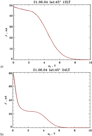
To demonstrate how well the proposed analytical solution may fit the current-voltage response in the multi-specious plasma, we consider two examples: both of them corre-spond to the plasma parameters that were found from the IRI model for the day 21.06.04 and the geographical altitude of 45◦. The first example is taken at sub-Sun point (12:00 LT), where plasma with the following parameters is expected to be observed, Ti = 0.19 eV, nO+ = 3·1010m−3, nHe+ =
nH+ = 109m−3(Fig. 3a), and the second one corresponds
to the midnight time (24:00 LT) withTi = 0.09 eV,nO+ =
1.6·1010m−3,nHe+ = 4·109m−3,nH+ = 3·1010m−3
(Fig. 3b). The satellite potential in both cases is assumed to be 0 V and the bulk velocity equals the satellite speed. The current-voltage response in such conditions was computed using the numerical code (black line) and then was fitted by the 1-D∗solution (red line). The precision of the parameters obtained from the fit is the following:1Ti ≈0.1%,1nO+≈
0.3%,1nHe+ ≈ 3%,1nH+ ≈ 3%,1vk ≈ 20 m s−1 and
1Ti ≈ 1%,1nO+ ≈ 1%,1nHe+ ≈ 10%, 1nH+ ≈ 2%,
(a)
(b)
(c)
Fig. 2. Current-voltage response of the APR analyser to O+(a), He+(b)and H+(c), withTi = 0.086 eV andni = 1010m−3, as computed using the numerical code (black line) and the 1-D∗ so-lution for the ion flux with the effective section of the entrance di-aphragm (red line). Green lines represent a 3-D analytical solution in which the losses of the particles are not taken into account.
(a)
(b)
Fig. 3. Current-voltage response in the multi-species plasma for the conditions, as predicted by the IRI model on 21.06.04 at the altitude of 45◦:(a)in sub-Sun point (12:00 LT), withTi=0.19 eV,
nO+=3·1010m−3,nHe+=nH+=109m−3, and(b)at midnight time (24:00 LT) withTi=0.09 eV,nO+=1.6·1010m−3,nHe+=
4·109m−3nH+=3·1010m−3. The numerical solution is given
by the black line and 1-D∗solution by the red line.
collected current is added to the received signal, then the precision is decreased, i.e. 1Ti ≈ 12%, 1nO+ ≈ 7%,
1nHe+ ≈ 50%, 1nH+ ≈ 50%, 1vk ≈ 30 m s−1 and
1Ti ≈ 2%,1nO+ ≈ 2%,1nHe+ ≈ 20%, 1nH+ ≈ 6%,
1vk = 50 m s−1 for 12:00 LT and 24:00 LT, respectively. However, this precision is still sufficient to resolve the main ion components.
3.5 Deviation of the ion velocity from the analyser axis Information about the component of the ion velocity transversal to the analyser axis may be deduced from the ADV measurements. The ADV collector consists of four identical sectors, a, b, c, d, which are connected by pairs (Fig. 4). The currents collected by the pairsa–c,b–d and a–b,c–dgive a possibility to reconstruct the deviation of the ion bulk velocity from thez-axis of the analyser along the axisxand the axisy, respectively.
Fig. 4. Four sectors of the ADV collector and their connections in pairs, as it is seen from the entrance diaphragm. The ratios of the currents collected by pairsa–c andb–d(left-hand panel) ora–b andc–d(right-hand panel) give a possibility to derive the deviation of the ion bulk velocity from the analyser’sz-axis along thex- or y-axis, respectively.
First, assume that plasma contains only one ion popula-tion. If the thermal velocity of ions,vT, is much less than
the component of the bulk velocity parallel to the analyser axis,vk, then the ion population may be considered as “cold” and the simple geometrical relation between the ratio of the currents collected by the pairs and the azimuthal,ϕ, and the co-latitudinal,θ, angles may be found. It reads
αx =(rd−htgθcosϕ)/(rd+htgθcosϕ), (12a)
αy =(rd−htgθsinϕ)(rd+htgθsinϕ). (12b)
Here,rd is a half-side of the entrance diaphragmg3, which
has the form of a square, his the distance between this di-aphragm and the collector (Fig. 1b),αx(αy)is the ratio of
the currents measured by the pairs a–c andb–d (c–d and a–b), θ is the angle between the ion bulk velocity (in the satellite frame) and z-axis, ϕ is the angle in thexy plane. Expressions (12 a, b) are valid when (i) both pairs collect the current and (ii) ion flux that enters in the diaphragm is en-tirely measured by the collector, i.e. whentgθ < rd/ hand
tgθ < (rc−
√
2rd)/ h, wherercis the radius of the collector.
For the ADV analyser, withh= 20 mm,rd= 15 mm andrc=
35.5 mm, the above mentioned conditions are satisfied when the co-latitudinal angle is less than 35.6◦.
(a)
(b)
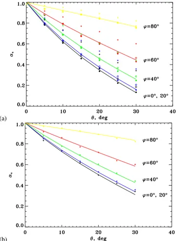
Fig. 5. (a)Ratio of the currents collected by opposite pairs,a–cand b–d, of the ADV collector as a function of the co-latitudinal angle of the ion flow, given for different values of the azimuthal angle. The temperature of the ion population is chosen to be 0.2 eV and the parallel velocity is 7.25 km s−1. Filled and open circles and crosses represent the results of the numerical calculation for O+, He+, H+, respectively. Solid lines show the behaviour which is predicted by the “cold plasma” approximation (12a). Black, blue, green, red and yellow colours are used to plot the analyser’s response for the ions flows with the different azimuthal angles, i.e. 0◦, 20◦, 40◦, 60◦ and 80◦. (b)Current ratio that is produced on the collector by the hydrogen flow (crosses) in the same plasma conditions as in (a). Solid lines show the behaviour that is fitted by Eq. (12a), in which the diaphragm’s half-size is replaced by its effective value,rd∗ = 22 mm.
the azimuthal angle. The temperature of the ion population is chosen to be 0.2 eV and the parallel velocity is 7.25 km s−1. Filled and open circles and crosses represent the results of the numerical calculations for oxygen, helium and hydrogen, respectively. Solid lines show the behaviour that is predicted by the “cold plasma” approximation (12a) and, as it is seen from the figure, perfectly fit the points that are attributed to He+and O+(open and filled circles), but not H+(crosses). The poor agreement of hydrogen is because its thermal veloc-ity is a significant fraction of the drift velocveloc-ity which reduces the current difference between the anode pairs. The current ratio produced on the collector by the hydrogen flow may be
Fig. 6.Effective size of the entrance diaphragm as a function of the ratio between thermal and bulk velocities.
fitted by the expression identical to Eqs. (12a, b), in which the diaphragm half-size,rd, is replaced by its effective value,
rd∗. For example, the current responses of the ADV sensor to the hydrogen flows (crosses in the Fig. 5a) are fitted by Eq. (12a) withrd∗ =22 mm (Fig. 5b). The effective size of the diaphragm is a function of the ratio between the thermal and the bulk velocities, and follows the empirical law rd∗=rd+c[VT/Vk]2, (13)
withc≈10 in the case of the ADV geometry (Fig. 6). Overall, in plasma with one ion species the measured ratio of currents gives a possibility to reconstruct the arrival angles of the ion flow. The angles may be estimated immediately from Eqs. (12a, b) and reads
tgθ =r
∗ d
h "
1−αx
1+αx
2 +
1−αy
1+αy
2#0.5
, (14a)
cosϕ =αx−1 αx+1
" 1−αx
1+αx
2 +
1−αy
1+αy
2#−0.5
, (14b)
withrd∗ = rd, if the measured ions are He+, O+, etc., and
withrd∗, given by Eq. (13), for H+.
Now consider a situation when plasma contains more than one ion population. From the previous considerations it fol-lows that the ratio of the currents that are expected to be col-lected by the ADV sensor depends only on the arrival angles of ion flows in the plasma without hydrogen. In the presence of hydrogen the measured ratio of currents is determined not only by the arrival angles, but also by the ratio between the thermal and bulk velocities and by the relative concentration of the ion species. In the multi-species plasma the current ratio may be written in the following form
Ax=
(1+κ)axαx∗+ax+κα∗x
(1+κ)+κax+α∗x
, (15a)
Ay=
(1+κ)ayαy∗+ay+κα∗y
(1+κ)+κay+α∗y
Here, κ is the relative concentration of hydrogen, κ = nH+/n,αx,αyandα∗x,α∗yare the ratios of the currents that
are produced on the collector by the ions with the relative masses mi/mH+ ≥ 4 , and by H+, if they are measured
separately. The combination of Eqs. (12) and (15) provides the solution for the arrival angles of the ion flow with the assumption that ions move with the same velocity. It reads tgθ= (1+κ)rdr
∗ d
(κrd+rd∗)h
" 1−Ax
1+Ax
2 +
1−Ay
1+Ay
2#0.5 , (16a)
cosϕ= Ax−1 Ax+1
" 1
−Ax
1+Ax
2 +
1 −Ay
1+Ay
2#−0.5
. (16b) However, the last assumption may break down in a collision-free plasma, because the streaming along the magnetic field may be different for different species and at different ener-gies. This will be true, for example, if there exists a field-aligned heat flux in the ion population. If this occurs, the arrival angles estimated from the ADV measurements will reflect the convective velocity of the major ion species, gen-erally either oxygen or hydrogen. In order to remove un-certainty in the interpretation of the analyser measurements, the access of hydrogen on the collector may be suppressed by applying the positive potential, +2 V, to the input grid,g2
(Fig. 1b).
4 Conclusions
The main idea of the present study was to provide and to jus-tify sufficiently simple analytical tools that may be used to derive the ion flows from the current measurements. It was proven that in the conditions that are expected to be observed during the Demeter mission, i.e. when the bulk plasma locity in the satellite frame is larger than the ion thermal ve-locity,
1. The current-voltage response measured by the APR analyser is fitted reasonably well by the 1-D solution in which the contribution of the ion thermal motion transversal to the analyser axis is taken into account by introducing an effective area of the entrance diaphragm;
2. Even a minor ion population may be resolved from the APR response;
3. The current ratio measured by the ADV sensor may be fitted by an expression that arises from the sim-ple geometrical considerations, in which the size of the entrance diaphragm has been replaced by its effec-tive value if the current on the collector is produced by the ions flows with the characteristic thermal velocities which consist of more than half of the bulk speed; 4. The combination of the APR and ADV measurements
provides a possibility to reconstruct the arrival angles of the ion flows in the multi-species plasma.
Acknowledgements. This work was supported by the contract
736/CNES/7621. We thank J.-J. Berthelier for useful discussions and acknowledge the engineers of CETP, M. Godefroy, Y. Rennard and F. Leblanc, who developed the IAP instrument.
Topical Editor M. Lester thanks a referee for his help in evalu-ating this paper.
References
Hanson, W. B., Sanatani, S., Zuccaro, D., and Flowerday, T. W.: Plasma measurements with the retarding potential analyser on OGO 6, J. Geophys. Res., 75, 5483–5501, 1970.
Hanson, W. B., Frame, D. R., and Midgley, J. E.: Errors in retard-ing potential analyzers caused by nonuniformity of the grid-plane potential, J. Geophys. Res., 77, 1914–1922, 1972.
Hanson, W. B., Sanatani, S., and Zuccaro, D.: The martian iono-sphere as observed by the Viking retarding potential analysers, J. Geophys. Res., 82, 4351–4363, 1977.
Knudsen, W. C.: Evaluation and demonstration of the use of re-tarding potential analysers for the measuring several ionospheric quantities, J. Geophys. Res., 71, 4669–4678, 1964.
Knudsen, W. C., Spenner, K., Bakke, J., and Novak, V.: Pioneer Venus orbiter planar retarding potential analyser plasma experi-ment, IEEE Trans. Geos. Rem. Sens., 1, 49–54, 1980.