www.clim-past.net/10/2081/2014/ doi:10.5194/cp-10-2081-2014
© Author(s) 2014. CC Attribution 3.0 License.
CREST (Climate REconstruction SofTware): a probability density
function (PDF)-based quantitative climate reconstruction method
M. Chevalier1, R. Cheddadi1, and B. M. Chase1,2
1Institut des Sciences de l’Évolution de Montpellier, UMR 5554, Centre National de Recherche Scientifique/Université Montpellier 2, Bat. 22, CC061, Place Eugène Bataillon, 34095 Montpellier, CEDEX 5, France
2Department of Archaeology, History, Culture and Religion, University of Bergen, P.O. Box 7805, 5020 Bergen, Norway Correspondence to:M. Chevalier ([email protected])
Received: 28 January 2014 – Published in Clim. Past Discuss.: 17 February 2014 Revised: 19 October 2014 – Accepted: 20 October 2014 – Published: 28 November 2014
Abstract. Several methods currently exist to quantitatively
reconstruct palaeoclimatic variables from fossil botanical data. Of these, probability density function (PDF)-based methods have proven valuable as they can be applied to a wide range of plant assemblages. Most commonly applied to fossil pollen data, their performance, however, can be lim-ited by the taxonomic resolution of the pollen data, as many species may belong to a given pollen type. Consequently, the climate information associated with different species cannot always be precisely identified, resulting in less-accurate re-constructions. This can become particularly problematic in regions of high biodiversity. In this paper, we propose a novel PDF-based method that takes into account the different cli-matic requirements of each species constituting the broader pollen type. PDFs are fitted in two successive steps, with parametric PDFs fitted first for each species and then a com-bination of those individual species PDFs into a broader sin-gle PDF to represent the pollen type as a unit. A climate value for the pollen assemblage is estimated from the likelihood function obtained after the multiplication of the pollen-type PDFs, with each being weighted according to its pollen per-centage.
To test its performance, we have applied the method to southern Africa as a regional case study and reconstructed a suite of climatic variables (e.g. winter and summer tem-perature and precipitation, mean annual aridity, rainfall sea-sonality). The reconstructions are shown to be accurate for both temperature and precipitation. Predictable exceptions were areas that experience conditions at the extremes of the regional climatic spectra. Importantly, the accuracy of the
reconstructed values is independent of the vegetation type where the method is applied or the number of species used.
The method used in this study is publicly available in a software package entitled CREST (Climate REconstruction SofTware) and will provide the opportunity to reconstruct quantitative estimates of climatic variables even in areas with high geographical and botanical diversity.
1 Introduction
Reconstructing past climates, while being an important ele-ment in the global effort to understand climate system dy-namics and their potential future structure and characteris-tics, is often limited to qualitative assessments of past con-ditions. This limits the potential for comparisons with the general circulation model (GCM) simulations, and the in-tegration of palaeoenvironmental information in modelling initiatives (Braconnot et al., 2012). As a result, while incon-sistencies exist both between GCM simulations and between GCM simulations and fossil records, it is difficult to use the bulk of the palaeodata available to evaluate GCM simulations in an efficient and effective way.
modern analogue technique (MAT) (Overpeck, 1985; Guiot, 1990), weighted averaging (WA) (ter Braak and Looman, 1986; ter Braak and van Dame, 1989; Birks et al., 1990), weighted averaging–partial least-squares regressions (WA-PLS) (ter Braak and Juggins, 1993), artificial neural networks (ANNs) (Malmgren et al, 2001) or regression trees (Salonen et al., 2012) – and (2) those based on plant distributions – mu-tual climatic range (MCR) (Atkinson et al., 1987; Sinka and Atkinson, 1999; Elias, 1997), the coexistence approach (CA) (Mosbrugger and Utescher, 1997; Utescher et al., 2014) or probability density functions (PDFs) (Kühl et al., 2002; Truc et al., 2013). These methods are fully detailed in Birks et al. (2010). Amongst these methods, MAT, WA and WA-PLS are the most commonly used. To date, no consensus has been reached as to which performs the best, and since the paper of Telford and Birks (2005) the debate has been focussed on the sensitivity of different methods to spatial autocorrelation in the training data set, which can cause an overestimation of the performance of a method (Telford and Birks, 2005, 2009, 2011b; Guiot and de Vernal, 2011a, b).
Beyond these conceptual issues, the calibration data set is another key concern. Methods based on plant assemblages need to be calibrated on robust modern data sets covering various environmental and biotic conditions, data sets that are not available from many parts of the world (e.g. drylands where pollen is often poorly preserved in surface samples). In such situations, the flexibility of methods based on plant dis-tributions (MCR, CA, PDFs) becomes more evident, expand-ing the range and scope of “reconstructible” environments. They also offer the possibility to reconstruct climate from non-analogue assemblages, provided that most species from that palaeoassemblage still exist. Conceptually, PDF-based methods evolved from MCR techniques as a way to model the strength of the relationship between plants and climate. Indeed, MCR (which considers a rectangular envelope de-fined by minimum and maximum values for a given climate variable) can be seen as the simplest PDF-based method. These methods are based on the correlation between plants’ modern geographical distribution and climate gradients, with the climate value that is the most common in the plant distri-bution being its “optimum”. Among the approaches that have already been proposed within the last decade (Kühl et al., 2002; Gebhardt et al., 2007; Truc et al., 2013), a recurrent is-sue concerns the assumptions made about the morphological characteristics of the envelope (width, skewness, central ten-dencies). Kühl et al. (2002) fitted a multidimensional Gaus-sian surface that excluded both multimodality and asymme-try, which are however common features when dealing with botanical assemblages. Later, Gebhardt et al. (2007) pro-posed to fit mixture models (combination of several Gaus-sian surfaces) to relax the constraints of a unimodal GausGaus-sian shape, and more recently Truc et al. (2013) proposed the ap-plication of non-parametric PDFs to improve the fit between PDF and data.
In addition to the issue of the shape, the accuracy of such models is also a function of the taxonomic resolution at which pollen can be identified (usually family to generic level) and the number of species making up a given pollen type. Pollen types often become climatically non-informative due to a saturation effect wherein too many species result in the climatic information conveyed by each species being averaged and lost. Contrary to the problem of the shape of the climate envelope, the problem of low taxonomic resolu-tion has rarely been discussed as its effects are usually not significant when plant diversity is relatively low. However, in areas where pollen types can comprise a high number of plant species (>30), it becomes increasingly significant and
can result in saturated PDFs. Truc et al. (2013) proposed a species selection method (SSM) that recursively alters the taxonomic composition of a pollen type by taking into ac-count the coexistence with other pollen types. In order to minimize PDF saturation, the SSM removes species that have climate requirements that are different from that of the as-semblage.
However, the SSM only removes species with optima at the extremes of climatic gradients, leaving a certain number of climatically undifferentiated species around the median climate. We believe that the problems of PDF shape and plant diversity are in fact intimately related to the strategy used for fitting PDFs. A pollen type is not a homogeneous ecolog-ical unit in the sense that many species with different cli-mate requirements can be classified in the same pollen type. From this point of view, fitting a density function directly to a pollen type is questionable. On the basis that species are the ecological units that respond to climate gradients, we propose a two-step procedure to define the PDF of the pollen types: (1) univariate and unimodal parametric PDFs are fitted for the species (PDFsp’s), and (2) those parametric PDFspare combined to produce the PDF of the pollen-type (PDFpol). The PDFpolreflects the diversity that exists among its species by considering independently each species. To reconstruct a climate value, we propose to combine the PDFpol with a weighted geometric mean. The multiplication of PDFpol en-sures the conservation of the mutual climatic range.
The method presented here has been implemented in a software package entitled CREST (Climate REconstruction SofTware). CREST – presented in Appendix A – is intended to make quantitative climate reconstructions more accessible to the wider community. Our hope is that a proliferation of quantitative reconstructions of past climate conditions will facilitate the consideration of palaeoenvironmental data in the assessment of GCM performance and ultimately allow for an improved understanding of both past and potential fu-ture climate change.
2 Methodology
The climate reconstruction method we propose is based on univariate PDFs. Here, a PDF represents the probability of a species existing along a climate gradient and is a surro-gate for the species’ realized niche (see for example Kear-ney, 2006). The process follows three general steps: (1) the plant–climate relationship is quantified (i.e. PDFs are fitted), (2) information conveyed by each taxon is combined and fi-nally (3) a climate value from the resulting climate likelihood function is extracted. This method relies on the assumption that the plant–climate relationship has remained relatively constant since the deposition of the fossil assemblage.
2.1 Fitting of the PDFs
This step is critical for all PDF-based methods. Many differ-ent strategies have been proposed (Kühl et al., 2002; Geb-hardt et al., 2007; Truc et al., 2013), all of them fitting a PDF to the pollen types identified in the fossil record. This strat-egy leads to a loss of certain information because (1) individ-ual signals are mixed and (2) rare species are masked by the most extended ones.
Here we propose a two-step procedure to fit PDFs that bet-ter integrates the diversity that can exist within some pollen types. First, we fit a PDF to each species (noted PDFsp), and secondly we combine the PDFspinto PDFpol. The latter con-siders more clearly the pollen type’s diversity.
2.1.1 Creating PDFsp
Based on observations, we propose that distributions of cli-matic values where a species is found – its niche – can be classified into two shapes: a log-normal shape (Fig. 1a) or a normal shape (Fig. 1b) (Austin, 1987; Austin and Gaywood, 1994; Hirzel and Le Lay, 2008). The normal shape is sym-metric, while the log-normal shape is markedly right-skewed (left-skewed distributions have been observed but are uncom-mon). In addition, the log-normal function is null for negative values, which is of interest when modelling variables such as rainfall amounts. Both curves are defined by two parameters: the mean xsp (Eq. 1) and the variance sx,2sp (Eq. 2) of the
species niche, withxbeing the studied climatic gradient.
The estimation ofxspands2x,spcan be biased if the
abun-dance of each climate value is not considered (Telford and Birks, 2011a). Following the model of Kühl et al. (2002) on that particular point, we propose dividing the climatic space into bins of equal width. All the climate values (a total ofN)
are sorted intoJbins. The number and/or length of the bins is
variable and depends on the dispersion of the climate values. A weightkj is defined for each bin as the ratio ofN with the
number of pixelsnj in the binj (Eq. 3). Each climate value
from binj will have the same weightkj.
xsp = P1
N i=1ki
N
X
i=1
kixi (1)
sx,2sp = P1
N i=1ki
N
X
i=1
ki(xi−xsp)2 (2)
kj =
N
nj
(3)
The shape and the position of the PDFspalong a gradient can be calculated with Eqs. (4) and (5) representing the normal law and the log-normal law (Fig. 1b and a), respectively.
PDFsp(x) = q 1
2π s2x,sp
exp −(x−xsp)
2 2sx,2sp
!
(4)
PDFsp(x) = √ 1
2π σ2x2exp
−(ln(x)−µ)
2 2σ2
(5)
with
µ=ln(xsp)−12 ln
1+s2x,sp
x2sp
σ2=ln
1+sx,2sp
x2sp
2.1.2 Creating PDFpol
To create the PDFpol, all the PDFsp’s are added with a weight determined by their geographical extent (represented by the number of grid cells occupiedni, Eq. 6). Due to the absence
of detailed, functional information regarding the pollen pro-duction of the different plant species, we are forced to con-sider that it is a constant among all the species of a pollen type and thus that each species is likely to have equally con-tributed to the observed pollen biomass. While PDFsp’s have an imposed shape, PDFpol’s are not constrained since no as-sumptions are being made. A PDFpolcan thus be multimodal when the diversity within the pollen type results in two or more climatically separated groups of species. Figure 1c and d highlight the advantage of that method: for instance, the cli-matic signals conveyed by the three speciesTribulus crista-tus,T. pterophorusandT. zeyheriare not masked by the sig-nals of the most extended one,T. terrestris.
PDFpol(x) = PspN1 sp1
√nsp i
spN X
sp1
p
clim[[i]][, 2]
Density
10 15 20 25
0.0
0.1
0.2
0.3
0.4
clim[[i]][, 2]
Density
10 15 20 25
0.0
0.1
0.2
0.3
0.4
Density
10 15 20 25
0.0
0.1
0.2
0.3
0.4
Density
10 15 20 25
0.0
0.1
0.2
0.3
0.4
d
Density
0 20 40 60 80
0.00
0.04
0.08
d
Density
0 20 40 60 80
0.00
0.04
0.08
Density
0 20 40 60 80
0.00
0.04
0.08
Density
0 20 40 60 80
0.00
0.04
0.08
Density
0 20 40 60 80
0.00
0.02
0.04
0.06
0.08
0.10
10 15 20 25
0.0
0.1
0.2
0.3
0.4
Tribulus cristatus (74) Tribulus pterophorus (89) Tribulus zeyheri (229) Tribulus terrestris (682) Pollen type Tribulus (1074)
Mean Annual Temperature (Tmean ann) Precipitation of the Dryest Quarter (Prec dry Q) Mean Annual Temperature (Tmean ann) A
C D
B
Precipitation of the Dryest Quarter (Prec dry Q)
Figure 1.An example of PDF fitting for two variables (Prec dry Q and Tmean ann) for the pollen typeTribulus, which is composed of four
species in our database. Four PDFsp’s are then fitted for each variable (aandb) and combined to create the PDFpol(candd). The dashed
lines on(c)and(d)are the PDFs obtained by Truc et al. (2013). The difference between the two methods is more marked for prec dry Q,
where (i) the PDFpolis null for negative precipitation values (more realistic) and (ii) the optimum is more marked and reflects the optima of
the different species.
2.2 Combination of the PDFpolto create the PDFvar
We propose the combination of different PDFpol’s with a weighted geometrical mean (Eq. 7). The multiplication of PDFpol’s ensures that the reconstructed climate value will be in the mutual climate range of the taxa considered. In addi-tion, since plants may pollinate more when they live close to their climate optimum (Birks and Seppä, 2004; Jackson and Williams, 2004), the PDFpol’s are weighted according to a monotonically increasing function of their pollen percentage
ωpol(s), withsrepresenting a sample (Eq. 8).
PDFvar(x, s) =
polYN pol1
PDFpoli(x) ωpoli(s)
polPN
pol1ωpoli(s)
!−1
(7) Using pollen percentagesppol(s)to weight taxa is
Cumulated 100-α% on both sides x(s)
Confidence Interval at α% x
Density of probability
Figure 2. Calculation of a CI exemplified with a right-skewed
PDFvar. More values are rejected on the right-hand side of the
cli-mate gradient. The grey areas cover an area representingα%.
and 1, with 1 corresponding to the highest percentage ob-served for the pollen type. This normalization is, however, very sensitive to outliers. In CREST, percentages are rescaled by the mean percentage of the pollen type when it is present in a sample. In other words, to calculate the mean, only strictly positive values are considered (Eq. 8). For a given pollen type, our weights have a correlation of 1 with those of Truc et al. (2013); the difference lies in the relative weights between taxa.
ωpol(s) = ppol(s)
mean(ppol(s))∀s,ppol(s)>0 (8)
2.3 Climate reconstruction
The reconstructed climate corresponds to the abscissa x(s)d of the optimum of PDFvar(Eq. 9). PDFvardescribes the like-lihood of any climatic value to be the target value when con-sidering the presence of many pollen types.
d
x(s) = argmax(PDFvar(x, s)) (9)
2.4 Error estimations
PDFvar’s provide access to the complete distribution of er-rors. They can be estimated at different thresholds (notedα).
Theα% confidence interval (CI) is more appropriate than a
standard deviation because PDFvar’s are rarely symmetrical (Fig. 2).
3 Validation
As a case study, we have used a modern botanical database to reconstruct a set of contemporary climate values to high-light and explore the strengths and weaknesses of the ap-proach, and to quantify its accuracy and robustness. Using southern Africa as a study area, we consider five countries:
Figure 3.Distribution of the southern African biomes and
ecore-gions (Olson et al., 2001): (1) deserts and xeric shrublands –
(1a) Kaokoveld Desert, (1b) Namib Desert, (1c) Namibian savanna woodlands, (1d) Succulent Karoo, (1e) Nama Karoo, (1f)
Kala-hari xeric savanna; (2)montane grasslands and shrublands– (2a)
Drakensberg altimontane grasslands and woodlands, (2b) High-veld grasslands, (2c) Drakensberg montane grasslands, woodlands and forests, (2d) Maputaland–Pondoland bushland and thickets; (3)
Mediterranean forests, woodlands and scrub– (3a) Albany
thick-ets, (3b) montane fynbos and renosterveld, (3c) lowland fynbos
and renosterveld; (4)flooded grasslands and savannas– (4a)
Zam-bezian halophytics, (4b) ZamZam-bezian flooded grasslands, (4c) Etosha
Pan halophytics; (5)tropical and subtropical grasslands,
savan-nas and shrublands– (5a) southern Africa bushveld, (5b) Kalahari
Acacia-Baikiaea woodlands, (5c) Zambezian and Mopane wood-lands, (5d) Angolan Mopane woodwood-lands, (5e) Zambezian Baikiaea
woodlands; (6)tropical and subtropical moist broadleaf forests–
(6a) Maputaland coastal forest mosaic, (6b) KwaZulu–Cape coastal
forest mosaic, (6c) Knysna–Amatole montane forests; (7)
man-groves. The dashed white lines delineate the different rainfall zones
as defined by Chase and Meadows (2007): the winter rainfall zone
(WRZ; >66 % winter rain), the summer rainfall zone (SRZ; <
33 % of winter rain) and the year-round rainfall zone (YRZ) in be-tween.
South Africa, Namibia, Lesotho, Swaziland and Botswana (from 17 to 34.5◦S and from 12 to 32.5◦E, Fig. 3). This
< 10
10−50 50−200200−500
< 10
10−50
50−200
200−500 > 500
< 10
10−50
50−200
200−500 < 10
10−50 50−200
200−500 > 500
10−50 50−200
200−500
> 500
Botswana (533)
Swaziland (25)
Lesotho (47) South Africa (1807) Namibia (977)
No data <10 10-50 50-200 200-500 >500
Figure 4. Distribution of the number of species (nsp) per grid
cell. The greener the grid cell is, the more species are available to reconstruct climate. No botanical information is available in the black grid cells. Species records are most abundant in South Africa, Swaziland and Lesotho.
3.1 Climate system
Most of southern Africa is dominated by summer rain-fall related to the seasonal dynamics of the Intertropical Convergence Zone (ITCZ) and the advection of moist tropical air masses off the Indian Ocean. Annual rainfall is highest along the eastern escarpment (∼1200 mm yr−1;
Hijmans et al., 2005; Mitchell and Jones, 2005) and de-creases westward. Conversely, in the Cape region (southern tip of Africa), most of the rain falls during the winter months as a result of frontal systems embedded in the southern westerlies (Tyson, 1986) and can reach annual totals of more than 900 mm yr−1. A complex mosaic of rainfall regimes are found at the boundary between those two systems: from year-round rainfall along the south coast of South Africa (>900 mm yr−1 distributed in more than 100 rain events
per year) to the super-arid Namib Desert (<20 mm, <10
rain events). The orographic effects of the Drakensberg escarpment and the Cape Fold Belt are very marked, creating a strong rain shadow effect in their lee.
The west coast is cooled by upwelling associated with the northward-flowing Benguela Current, whereas the south and east coasts are warmed by the southward-flowing Agulhas and Mozambique currents, respectively. At a given latitude, the difference in temperature between the two coasts can ex-ceed 6◦C. The greatest diurnal temperature ranges are found
in the interior, especially in the Kalahari and the Karoo re-gion, where the altitude is greater than 1000 m a.s.l.in many
areas (Hijmans et al., 2005).
The study region currently supports four primary biomes: deserts and xeric shrublands (54.7 %); montane grasslands and shrublands (16.8 %); tropical and subtropical grass-lands, savannas and shrublands (25.3 %); and Mediterranean forests, woodlands and scrub (3.2 %) (Olson et al., 2001). The latter is better known as the Cape Floristic Region, which is dominated by the Fynbos Biome. Each biome is divided into ecoregions (Fig. 3), which will be used to describe the model’s properties.
3.2 Data
We have extracted botanical data for all grid cells where at least one plant with more than 25 pixels in its distribution had been recorded, leading to a total of 3389 “samples” (Fig. 4). We have then selected 20 climatic variables of interest: 9 temperature-like and 11 moisture-like variables (Table 1). A total of 4969 species distributions have been used.
3.2.1 Botanical data
Botanical data were extracted from a series of databases held by the South African National Biodiversity Institute (SANBI, 2003; Rutherford et al., 2003, 2012). The data from these sources, which are derived mainly from herbarium col-lections and documented observations, are most commonly available as “presence” within a particular 0.25◦×0.25◦grid
square. We have used this resolution for our analyses, upscal-ing more precisely located data to this common resolution. Data were obtained from field surveys performed during the late twentieth century, between 1970 and 2000 with a peak in the 1980s.
In this study, we only consider species with at least 25 oc-currences, resulting in a number of species (nsp) available per
pixel between 1 and 1371 (median=47). This strong het-erogeneity is mainly due to both the range of environments found in our study area (Fig. 3) and the strong difference that exists between the different countries (Fig. 4), with South Africa providing by far the most extensive data set.
3.2.2 Climatic data
To define PDFs, the species distributions have to be associ-ated with climate data. For this study we have reconstructed 20 climate variables from our data set. While some of those variables represent climatic features playing a strong role in a plant life cycle (e.g. number of frost days or different precip-itation variables), the impact of some others is much more indirect (e.g.mean diurnal rangeor temp ann range). The purpose of this strategy is to assess the extent to which dif-ferent climate variables can be reliably reconstructed with CREST.
Table 1.List of the 20 climate variables reconstructed for southern Africa (name, description and original reference).
Variable’s name Description Reference
Temperature Tmean ann Mean annual temperature Hijmans et al. (2005)
Mean diurnal range Mean of monthly (max temp–min temp) Hijmans et al. (2005)
Temp seasonality Standard deviation of the annual temperature (×100) Hijmans et al. (2005)
Temp ann range Annual range of temperature (max–min) Hijmans et al. (2005)
Tmean wet Q Mean temperature of the wettest quarter Hijmans et al. (2005)
Tmean dry Q Mean temperature of the driest quarter Hijmans et al. (2005)
Tmean warm Q Mean temperature of the warmest quarter Hijmans et al. (2005)
Tmean cold Q Mean temperatures of the coldest quarter Hijmans et al. (2005)
Frost days Number of frost days per year Mitchell and Jones (2005)
Moisture Prec ann Annual precipitation Hijmans et al. (2005)
Prec seasonality Coefficient of variation of annual precipitation Hijmans et al. (2005)
Prec wet Q Precipitation of the wettest quarter Hijmans et al. (2005)
Prec dry Q Precipitation of the driest quarter Hijmans et al. (2005)
Prec warm Q Precipitation of the warmest quarter Hijmans et al. (2005)
Prec cold Q Precipitation of the coldest quarter Hijmans et al. (2005)
SWC winter Soil water content during winter Trabucco and Zomer (2010)
SWC summer Soil water content during summer Trabucco and Zomer (2010)
Aridity Mean annual aridity index (×10 000) Trabucco and Zomer (2009)
WRP Percentage of winter rainfall Derived from Hijmans et al. (2005)
Wet days Number of rain days per year Mitchell and Jones (2005)
elements in studying the eco-physiological tolerance of plants species. These data were then upscaled to match the resolution of the botanical data (0.25◦×0.25◦). Additional
variables of interest have also been derived from WORLD-CLIM’s data, including the soil water content (SWC; Tra-bucco and Zomer, 2010) for both summer and winter, the mean annual aridity (Trabucco and Zomer, 2009) and winter rainfall percentage (WRP). We have also used two variables from the CRU 2.10 (Climate Research Unit) data (Mitchell and Jones, 2005): the number of frost and wet days during the year. Those data (0.5◦×0.5◦grid cells) were downscaled
to meet our resolution. All the climatic values used in this study are representative of the period 1960–1990; the period is extended to 1950–2000 in some situations.
The description of all variables as well as their original reference is summarized in Table 1.
4 Results
4.1 Accuracy of the model
We have measured the climate anomaliesδv(s)for each
sam-plesand each variablevbetween the reconstructed climate
Reconv(s) and the instrumental value Instruv(s)according
to Eq. (10). A positive/negative anomaly is equivalent to an under/overestimation of the targeted climate.
δv(s)=Instruv(s) − Reconv(s) (10)
The dispersion of the anomalies for each variable was cal-culated with the R software (as all the statistics presented
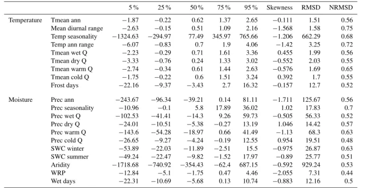
here; R core team, 2014) and has been compiled in Table 2. The distributions of anomalies are all centred around 0. Even if all the median values are statistically different from 0 (sign test,p <10−5), the relatively low value of these
me-dians indicates that the model is not subject to undue bias. A major dichotomy can be observed between the two types of variables (χdf2
=1 test with Yates’ continuity correction, p=1.8×10⁻³): for the temperature-like variables, the
me-dian is positive for eight out of nine variables (general under-estimation), while for moisture-like variables the opposite is observed, with negative medians for 10 out of 11 variables (general overestimation, Table 2). The different percentiles we have calculated provide insight regarding the dispersion of the reconstructed values, as do the histograms in Fig. 10. The skewness is most often negative (for 14 variables), mean-ing that when errors are negative (overestimation) their abso-lute value is higher than when they are positive (75 and 95 % percentiles respectively higher than the 25 and 5 %).
The root mean square deviation (RMSDv; Eq. 11) is an
index that reflects the mean error of a model, but it is sensitive to outliers. It does, however, allow for a good evaluation of the performance of the model. All the values are compiled in Table 2.
RMSDv =
v u u t1
N N
X
s=1
δv(s)2 (11)
The amplitude of δv(s) and RMSDv are functions of the
Table 2.Summary of the dispersion of the anomaliesδv(s)(5, 25, 50, 75 and 95 % quantiles), skewness, RMSD and NRMSD of each variable. The medians are statistically different from 0.
5 % 25 % 50 % 75 % 95 % Skewness RMSD NRMSD
Temperature Tmean ann −1.87 −0.22 0.62 1.37 2.65 −0.111 1.51 0.56
Mean diurnal range −2.63 −0.15 0.51 1.09 2.16 −1.568 1.58 0.75
Temp seasonality −1324.63 −294.97 77.49 345.97 765.66 −1.206 662.29 0.68
Temp ann range −6.07 −0.83 0.7 1.9 4.06 −1.42 3.25 0.72
Tmean wet Q −2.23 −0.29 0.71 1.61 3.36 0.455 1.99 0.56
Tmean dry Q −3.33 −0.76 0.24 1.33 3.02 −0.552 2.03 0.55
Tmean warm Q −2.74 −0.34 0.61 1.44 2.63 −0.576 1.69 0.65
Tmean cold Q −1.75 −0.22 0.6 1.51 3.24 0.392 1.7 0.55
Frost days −22.16 −9.37 −3.43 2.7 16.32 −0.157 12.7 0.52
Moisture Prec ann −243.67 −96.34 −39.21 0.14 81.11 −1.711 125.67 0.56
Prec seasonality −10.96 −0.1 5.8 17.89 36.02 1.02 17.83 0.7
Prec wet Q −102.53 −41.41 −14.3 9.26 59.73 −0.505 56.33 0.52
Prec dry Q −24.01 −10.51 −5.38 −0.27 13.19 1.046 14.42 0.57
Prec warm Q −143.6 −54.28 −18.97 0.66 41.49 −1.13 68.3 0.63
Prec cold Q −26.65 −9.27 −4.24 −0.19 12.55 0.954 19.51 0.48
SWC winter −53.89 −22.03 −11.89 −2.51 15.5 −0.975 26.87 0.63
SWC summer −49.24 −22.47 −9.82 −1.52 17.97 −0.89 25.77 0.51
Aridity −1718.68 −740.92 −354.43 −62.4 687.15 −0.592 929.24 0.53
WRP −12.84 −5.1 −1.75 0.47 4.46 −2.055 7.31 0.44
Wet days −22.31 −10.69 −5.68 0.13 10.74 −0.883 12.16 0.5
of variation, such as Tmean ann, Tmean cold Q and Tmean warm Q. To remove this discrepancy, we have normalized our RMSDs by the observed standard deviation of the in-strumental values (NRMSDv; Eq. 12). NRMSDs are lower
for moisture-like variables, whilst they exhibit the highest anomalies (in units of NRMSD; Figs. 6 and 7). Four vari-ables present a high NRMSD: mean diurnal range (0.75), temp ann range (0.72), prec seasonality (0.70) or temp sea-sonality (0.68). The climatic signal of these four variables does not seem to be well captured by the botanical data, and plant distribution is apparently not directly driven by those variables. They represent annual climatic variability, and a range of climatic scenarios could result in the same values. For example, the variable prec seasonality takes identical val-ues for seasonal rainfalls whether they occur mainly in winter or summer. This major difference is incorporated into WRP, which has been reconstructed with a much better accuracy (NRMSD=0.44).
NRMSDv =
RMSDv σInstru,v
(12)
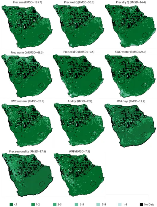
4.2 Geographical analysis of the errors
Generally, southern African climates are accurately recon-structed with CREST. The anomalies that do exist are not randomly dispersed throughout the study area. On the con-trary, regions of enhanced or diminished error are observed for each variable (Figs. 5 and 6). On these figures, anomalies have been normalized by the RMSD (Eq. 13) to make all the
maps comparable.
δnorm,v(s) =
δv(s)
RMSDv
(13)
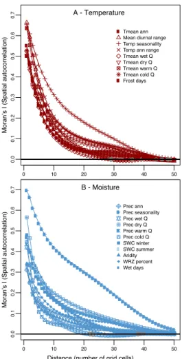
This observation is validated with the measure of the spatial autocorrelation of the anomalies with Moran’s I (Moran, 1950) (Eq. 14 and Fig. 7). This index measures the (dis)similarity of nearby locations in space. To compute this index, a neighbourhood matrix of weightswis defined. We
have measured the spatial autocorrelation at different dis-tances: from a local perspective, where only adjacent grid cells are neighbours, to the continental scale, where all the grid cells are considered neighbours. Under the null hypoth-esis (no spatial autocorrelation), Moran’s I is normally dis-tributed. However,δv(s)is not, and mean and standard
de-viations were estimated empirically with 999 permutations for this vector. We ran 50 tests for each variables (one for each distance) and applied a Bonferroni correctionα=050.05.
Most of the tests were highly significant (blue and red dots in Fig. 7).
I = P N
i
P
jwij
P
i
P
jwij(vi−v)(vj−v)
P
i(vi−v)2
(14)
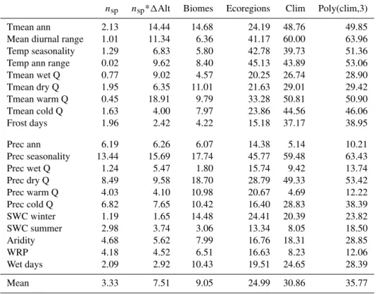
Table 3.Percentages of variance (R2) explained for the three different hypotheses we tested in this study to describe the distribution ofδv(s),
namely the impact of (1) the number of species (nspandnsp*1Alt), (2) the type of vegetation (biomes and ecoregions) and (3) the expected
climatic value (clim and poly(clim, 3)).
nsp nsp*1Alt Biomes Ecoregions Clim Poly(clim,3)
Tmean ann 2.13 14.44 14.68 24.19 48.76 49.85
Mean diurnal range 1.01 11.34 6.36 41.17 60.00 63.96
Temp seasonality 1.29 6.83 5.80 42.78 39.73 51.36
Temp ann range 0.02 9.62 8.40 45.13 43.89 53.06
Tmean wet Q 0.77 9.02 4.57 20.25 26.74 28.90
Tmean dry Q 1.95 6.35 11.01 21.63 29.01 29.42
Tmean warm Q 0.45 18.91 9.79 33.28 50.81 50.90
Tmean cold Q 1.63 4.00 7.97 23.86 44.56 46.06
Frost days 1.96 2.42 4.22 15.18 37.17 38.95
Prec ann 6.19 6.26 6.07 14.38 5.14 10.21
Prec seasonality 13.44 15.69 17.74 45.77 59.48 63.43
Prec wet Q 1.24 5.47 1.80 15.74 9.42 13.74
Prec dry Q 8.49 9.58 18.70 28.79 49.33 53.42
Prec warm Q 4.03 4.10 10.98 20.67 4.69 12.22
Prec cold Q 6.82 7.65 10.42 16.40 28.83 38.39
SWC winter 1.19 1.65 14.48 24.41 20.39 23.82
SWC summer 2.98 3.74 3.06 13.34 8.05 18.50
Aridity 4.68 5.62 7.99 16.76 18.31 28.85
WRP 4.18 4.52 6.51 16.63 8.23 12.06
Wet days 2.09 2.92 10.43 19.51 24.65 28.39
Mean 3.33 7.51 9.05 24.99 30.86 35.77
on the local scale than precipitation anomalies (higher values at distances lower than seven–eight grid cells), but the corre-lation decreases faster with distance (no distinction beyond 15 grid cells). Seasonality of temperature and precipitation have a distinct pattern, being correlated at longer distances, highlighting – in association with high NRMSDs (Table 2) – that their errors are not limited to distinct regions.
Four areas present a group of outliers for several vari-ables: (1) the Namibian coast (for temperature and precipi-tation), (2) the high mountains of Lesotho (for temperature and humidity variables), (3) the eastern part of the Great Es-carpment (precipitation) and (4) the southern coast of South Africa (precipitation) (Figs. 5 and 6).
4.3 Factors impacting the reconstructions
As the errors are spatially clustered, we have looked for fac-tors that could explain this distribution. There is no clear lin-ear relation between the anomalies absolute values andnsp.
The slopes of the linear models we fitted were statistically significant at the 5 % threshold but theR2were always low
(3.3 % of variance explained on average, Table 3). The mod-els can, however, be biased by the uneven distribution ofnsp;
half of the grid cells were reconstructed with 47 or fewer species, while some others were reconstructed with more than 1000 (Fig. 4). Some of our clusters of errors are found in mountainous regions, and we have hypothesized that the
errors may arise from a mix of low- and high-altitude plants, with the anomalies observed being proportional to the degree of mixing. Thus, we have calculated the intra-pixel variation of altitude (the standard deviation of all the 30 arc-second altitude values in each quarter-degree grid cell, later called
1Alt). We fitted linear models to explain the anomalies as
a function ofnsp and1Alt. However, the gain of explained
variance was relatively small (+0.9 % on average). These re-sults indicate that the anomalies are not a result of the number of species used for the reconstruction.
Figure 5.Geographical distributions of the normalized anomalies of the reconstructions of temperature-like variables (Eq. 13). The scale is
identical for all the maps, in units of RMSD. No vegetation information was available from the black pixels.
The between-groups PCA run on ecoregions explains 25 % of the total variance, but this is low relative to the number of groups (25). Again, more variance remained within the groups than between them. Figure 9 summarizes the mean dispersion of errors within each ecoregion. Some ecoregions appear to concentrate outliers, but these are always composed of 25 or fewer samples (low geographical extension and/or low amount of botanical data). Thus, despite the high botan-ical diversity that exists in southern Africa, we were not able to demonstrate the type of vegetation (forests, grasslands, sa-vannas, etc.) having any effect on the quality of the recon-structions.
The only factor that explains a significant part of the dis-persion is the distance of the expected value from the most represented value of the variable over the study area (Ta-ble 3). We fitted linear models to explain the anomalies as a function of the expected value (Fig. 10). All were
signifi-cant (pvalue<0.001) with positive slopes. A noticeable
dif-ference between temperature-like (R2=42 % on average)
and moisture-like variables (R2=22 % on average) is
ob-served, indicating that values that lie far from the most rep-resented climate exhibit the highest anomalies (on the left and/or right-hand side(s) on thexaxes in Fig. 10).
5 Discussion
Figure 6.Geographical distributions of the normalized anomalies of the reconstructions of moisture-like variables (Eq. 13). The scale is identical for all the maps, in units of RMSD. No vegetation information was available from the black pixels.
variables such as mean diurnal range or temp seasonality on the plant life cycle is indirect. Thus, they are less likely to be accurately reconstructed from pollen data. Variables that are surrogates for direct gradient may show strong ability to de-scribe modern data but poor predictive power to dede-scribe past conditions (see, e.g., the palaeolimnological example of Jug-gins, 2013). Selection of variable(s) of interest should always be conditioned to an appropriate analysis of the data. Statis-tics could help in that process (Mac Nally, 2000; Telford and Birks, 2011c), but the final decision about the variables to reconstruct should always derive from an enlightened choice based on both statistical and ecological/environmental
con-siderations. In the semi-arid to arid environments of southern Africa, precipitation and/or water availability strongly con-strain plants distributions, which probably explains why we get lower NRMSDs for moisture-related variables in our case study.
0 10 20 30 40 50
0.0
0.1
0.2
0.3
0.4
0.5
0.6
0.7
Tmean ann Mean diurnal range Temp seasonality Temp ann range Tmean wet Q Tmean dry Q Tmean warm Q Tmean cold Q Frost days
0 10 20 30 40 50
0.0
0.1
0.2
0.3
0.4
0.5
0.6
0.7
Prec ann Prec seasonality Prec wet Q Prec dry Q Prec warm Q Prec cold Q SWC winter SWC summer Aridity WRZ percent Wet days
B - Moisture A - Temperature
Distance (number of grid cells)
Moran’s I (Spatial au
tocorrelation)
Moran’s I (Spatial au
tocorrelation)
Figure 7.Moran’s I autocorrelogram. The spatial autocorrelation
is plotted for each variable against different distances (measured in grid cells). Each grid cell is about 28km large/high. Grey
sym-bols represent non-significant values; α=0.001 after the
Bonfer-roni correction. Only 17 out of 1000 tests are non-significant.
(estimation based on Fig. 9) in order to adequately determine the plant–climate relationship.
While our expectation was that a high number of species would result in more precise reconstructions, we were not able to observe any relationship between anomalies and the number of species. Anomalies do decrease when the number of species begins to increase (from 1 to∼20–30), but then
the tendency is reversed, and the large anomalies were ob-served in samples with the largest number of species. This may be related to a saturation problem, wherein more is not necessarily better. As we used a presence/absence weight-ing strategy, species far from their climate optimum have the same importance as those living in their optimal climate. The increase in the number of species could increase these marginal elements, biasing the reconstructions. The role of the number of taxa on the accuracy is not yet fully under-stood and is the subject of ongoing studies.
Other studies (Kühl et al., 2002; Scott et al., 2003; Truc et al., 2013) have shown that selecting a subset of the
−2
−1
0
1
2 1 - Deser
ts & X eric Shrublands
2 - Mon
tane Gr
asslands & Shrublands
3 - Medit
erranean F orests
,
Woodlands & S crub
4 - Flooded Gr
asslands & S avannas
5 - Tropical & Subtr
opical Gr asslands
,
Savannas & Shrublands6 - Tropical & Subtr
opical M oist
Broadleaf F orests
7 - Mang
roves
Figure 8.Box plots representing the dispersion of the normalized
anomalies (Eq. 13) for each biome. There is more dispersion within each biome (length of the boxes) than between, confirming the re-sults of the between-groups PCA (90 % of variance not explained by the groups).
−2
−1
0
1
2 1a - K aoko
veld deser t
1b - Namib deser t
1c - Namibian sa vanna w
oodlands
1d - Suc culen
t Kar oo
1e - Nama K aroo
1f - K alahar
i xer ic sa
vanna
2b - H igh
veld g rasslands
2c - Drakensber
g mon tane g
rasslands , woodlands and f
orests
2d - M aputaland-P
ondoland bushland and thickets
3a - A lban
y thickets
3b - M ontane fynbos and r
enost erveld
3c - L
owland fynbos and r enost
erveld
4a - Zambezian haloph ytics
4b - Zambezian flooded g rasslands
4c - E tosha P
an haloph ytics
5a - S outher
n A frica bush
veld
5b - K alahar
i Acacia-Baik iaea w
oodlands
5c - Zambezian and M opane w
oodlands
5d - A ngolan M
opane w oodlands
5e - Zambezian Baik iaea w
oodlands
6a - M aputaland c
oastal f orest mosaic
6b - K waZ
ulu-Cape c
oastal f orest mosaic
6c - K ny
sna-Ama tole mon
tane f orests
7 - Souther n A
frica mang roves
2a - Dr akensber
g alti-mon tane g
rasslands and w oodlands
** ** * ** * ** ** ** ** **
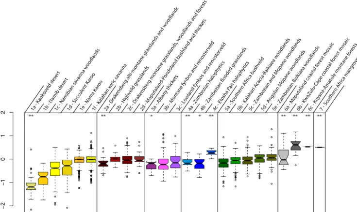
Figure 9.Box plots representing the dispersion of the normalized anomalies (Eq. 13) for each ecoregion. There is globally more dispersion
within each ecoregion (length of the boxes) than between, confirming the results of the between-groups PCA (75 % of variance not explained
by the groups).∗means the ecoregion is composed of fewer than 50 grid cells;∗∗means fewer than 25. The numbers match those of Fig. 3.
of interest (Juggins, 2013), so that only part of the recon-structed palaeovariability can be related directly to it. CREST (Appendix 1) provides a range of outputs that indicate the sensitivity of different taxa to given climatic parameters and allow the user to assess the data being considered and make informed choices in the selection of such subsets.
When plotted on a map (Figs. 5 and 6), the reconstruction anomalies appear to be spatially clustered. Those patches of large anomalies can be explained by the position of the local climate along the climate gradients (Fig. 10) and are a direct consequence of the hypotheses underlying the model. The method is correlative, and consequently it is biased towards the best-represented climate values. This uneven sampling of the environmental gradients biases the estimation of plants’ optima by shifting the “real” optimum towards the portion of the gradient with the most observations (Telford and Birks, 2011a). In most cases, lowest/highest values along the stud-ied climate gradient are rare, but there are exceptions. For ex-ample, low rainfall amounts are common in southern Africa, and as a result they are well represented and the signal is easily captured by the model.
To offset the impact of the climate distribution’s hetero-geneity, we upweighted rare climate values as proposed by Kühl et al. (2002) and Truc et al. (2013). This method shifts PDF optima towards the rarest climate values. The climate
abundance weighting did decrease the errors for the extreme climates but also increased them for the most common ones (data not shown). The overall impact is nevertheless positive since it decreased the RMSDs for all the variables. It also reduced the clustering of errors. Despite its advantages, the strategy has the drawback that artificial geographical limits must be selected (e.g. mountain ranges or country borders; Kühl et al., 2002) to compute the weights. A finite number of grid cells must be selected and sorted into bins. Any change in the boundaries would affect – potentially significantly – the weights, and thus the reconstructions. It is also possible that the climate abundance weighting may be the cause of the small but significant bias observed between temperature and moisture variables, which are, respectively, under- and overestimated for rare climates in the region.
Figure 10.Anomalies plotted against their expected values. The density of points is heterogeneous: being very dense around the median
climate and sparser at the extremes. This is illustrated by the histograms that represent the marginal distributions. The anomalies are smaller for the best-represented climate values and increase with distance from the median climate. The blue line represents the linear model fitted,
with its associatedR2.
the high mountains of Lesotho, where temperatures are very low and precipitation is high; (3) the thin coastal band along the southern coast of South Africa, where moist forests can develop as a result of significant aseasonal rainfall; and (4)
5 10 15 20 25 0 500 1000 ● ● ● ● ● ● ● ● ● ● ● ● ● ● ● ● ● ● ● ● ● ●● ● ● ● ● ●●●●●●● ● ● ● ● ● ●● ● ● ● ● ● ● ● ● ●● ● ● ● ● ● ●●●● ● ● ● ● ●● ● ● ● ● ● ●●●●● ● ● ● ● ● ● ● ● ● ● ● ● ● ● ● ●● ● ● ● ● ● ● ● ● ● ● ● ● ● ● ● ● ● ● ● ● ● ● ● ● ●● ●●●● ● ● ● ● ● ● ● ● ● ● ● ● ● ●● ● ● ● ● ● ● ● ● ● ● ● ● ● ●●● ● ●●●● ● ● ●●●● ● ● ● ● ● ● ● ● ●● ● ● ●● ●● ●● ● ● ● ● ● ●● ● ● ● ● ●●● ● ● ● ●●● ● ●● ●●● ● ● ● ● ● ● ● ● ● ● ● ● ● ●●● ● ● ● ● ● ● ● ● ● ● ●● ● ● ● ● ● ● ● ● ● ● ● ●●● ● ● ● ● ● ● ● ●● ●● ●● ●● ●●● ● ● ● ● ● ● ● ● ● ● ● ● ●●●● ● ● ●●●●● ●●● ● ● ● ● ● ● ● ●● ●●● ●● ● ● ● ● ● ● ● ● ● ● ● ● ● ●● ●●●●● ● ● ● ● ● ● ● ●● ● ● ● ● ● ● ● ●● ● ● ● ● ● ● ● ● ●● ● ●●●●● ● ● ●●●● ●●●●●●●●●● ● ● ● ● ● ● ●●●● ● ● ● ● ● ● ● ● ● ● ● ●●●●●●●● ●●●●●●●●●●●● ● ● ● ● ● ●●● ● ● ● ● ● ● ● ●●● ● ● ● ●●●●●●●●●●●●●●● ● ● ● ● ● ● ● ● ● ● ● ● ● ● ● ● ● ● ●● ●●●● ●●●●●●●●●●●●●● ●●●●●●●●●● ● ● ● ● ● ● ● ●●● ● ● ● ● ● ● ● ●● ● ● ●●●●●●● ●●●●●●●●●●●●●●●●●●●●●● ● ● ● ● ● ● ●● ● ● ● ● ● ●● ● ●● ●●● ● ●● ●●●● ● ● ● ● ● ● ● ● ● ● ● ● ● ● ● ● ● ● ● ● ● ● ● ● ●●● ● ● ● ● ●●●●●●●●●●● ● ● ● ● ● ● ●● ● ● ● ● ● ● ● ● ● ●● ● ●● ● ● ● ● ● ● ●● ● ● ● ●● ● ●● ● ● ● ● ● ● ●●● ● ● ● ● ●● ● ● ● ● ● ● ● ● ●● ● ● ● ● ● ●● ● ● ●●● ●●●●●●● ● ● ● ● ●● ● ● ● ● ● ● ● ●● ● ● ● ● ● ● ● ● ● ● ●● ● ● ● ● ●●●● ●●●● ●●● ●●●● ● ● ● ● ● ● ● ● ● ● ●● ● ● ● ● ● ● ● ● ●● ● ● ● ● ●● ●●● ●●●●●● ● ● ● ● ● ●● ●● ● ● ● ● ● ● ● ● ● ● ● ● ● ● ● ● ●●●●●●●●●●●●●●●●●●●●●● ● ● ● ● ● ● ●●●● ●● ● ● ● ● ● ● ● ● ● ● ●● ● ● ●● ● ● ● ● ●● ●●● ●●●●●●●●●●●●●● ● ● ● ● ● ● ● ● ●● ●● ● ●● ● ● ● ● ●● ● ● ● ● ● ● ● ● ● ●●● ● ● ●●● ● ●● ● ●●●●●●● ● ● ● ●● ● ● ● ● ● ● ●● ● ● ● ● ● ● ● ● ● ● ● ● ● ● ● ● ● ● ● ● ● ● ● ● ● ● ● ● ●●●●● ● ● ● ● ● ● ● ●● ● ● ● ● ● ● ● ● ● ● ● ● ● ● ● ● ● ● ● ● ●● ● ●●● ●●● ●●●●●●●●●●●●●●●●●● ● ●●● ●● ● ●● ● ● ● ● ● ● ● ● ● ● ● ● ● ● ● ● ● ● ● ● ● ● ● ● ● ●●●●●●●● ●● ● ●● ●●●● ●●●●● ●●●●●● ● ● ● ● ● ● ● ● ● ● ● ● ● ● ● ● ● ● ● ● ● ● ● ● ● ● ●● ● ● ● ●● ● ●●●● ● ● ●● ●● ● ● ● ●●●●● ●●● ● ● ● ● ● ● ● ● ● ● ● ● ● ●● ● ● ● ● ● ● ● ●●●●●●●● ●●●●●●●● ● ● ● ● ●● ● ● ● ● ● ● ● ● ● ● ● ● ● ● ● ● ● ● ● ● ● ● ● ● ● ● ●●●●●●●●●● ●●●●●●●●●● ● ● ● ● ● ● ● ● ● ● ●●● ●● ● ● ● ● ● ● ● ● ● ●● ● ● ● ● ● ● ●●● ● ● ● ● ● ● ● ● ●●● ● ● ● ●●●● ●●●●●●●●●● ● ● ● ● ●●● ●●● ● ● ● ● ● ● ● ● ●● ● ● ● ● ● ● ● ● ●●● ● ● ● ● ●● ● ●●● ● ● ●● ●● ● ● ● ● ● ●●●● ● ● ● ● ● ● ● ● ● ● ● ● ●● ● ● ● ● ● ● ● ● ● ● ● ● ● ● ● ● ● ●●● ● ● ●●●● ● ● ●● ● ● ● ● ● ● ● ● ● ● ● ● ● ● ● ● ● ● ● ●● ● ● ● ● ● ● ● ● ● ● ● ● ● ● ● ● ● ● ● ●●●● ● ● ● ● ● ● ● ● ● ●● ● ● ●● ● ● ● ● ● ● ●● ● ● ● ● ● ● ● ● ● ● ● ● ● ● ● ● ● ● ● ● ● ● ● ● ● ● ● ●●● ● ● ● ● ● ● ● ● ● ● ● ● ● ●● ● ● ● ● ●●● ● ● ● ● ●● ● ● ● ● ● ● ● ● ● ● ● ● ● ● ●● ● ●● ● ● ● ● ● ●●●● ● ● ● ● ● ● ● ● ● ● ● ● ● ● ● ● ●● ● ● ● ● ● ● ● ● ● ● ● ● ● ● ● ●● ● ● ● ● ● ● ● ● ● ●●●●●● ●●●●● ● ● ● ● ● ● ●● ● ● ● ● ● ● ● ● ● ● ● ●● ● ● ● ● ● ● ● ● ● ● ● ● ● ● ● ● ● ● ● ● ● ●● ● ● ● ● ● ●●●●●●●● ●●●●● ● ● ●● ● ● ● ● ●● ● ● ● ● ● ● ● ●● ● ● ● ● ● ●● ● ● ●● ● ● ● ● ● ● ● ●● ● ● ●● ● ● ● ● ● ● ● ● ●● ● ● ● ● ●●●● ● ● ● ● ● ● ● ● ● ● ● ● ● ● ● ● ● ●● ● ●●●● ● ●●● ● ● ● ● ● ● ● ● ●●● ● ● ● ● ● ● ● ●● ●●●●●● ● ● ● ●●● ● ● ● ● ● ● ● ● ●●● ● ● ● ● ● ● ● ●●● ●● ● ● ● ●● ● ● ● ● ● ● ● ● ● ● ● ● ● ● ● ● ● ● ● ● ●● ●●●● ●●●●●●●●●●●●● ● ● ● ● ● ● ● ● ● ●●● ● ● ● ● ● ● ● ● ● ● ● ● ● ● ● ● ● ● ● ● ● ● ● ● ● ● ● ● ● ● ● ● ●●● ● ● ● ● ● ● ● ● ● ● ● ●● ●● ● ● ● ● ● ● ● ● ● ●● ● ● ● ● ●● ● ● ●● ● ● ●●● ● ● ● ● ● ● ● ● ● ● ● ● ● ● ● ● ● ● ● ● ● ● ● ● ● ● ● ● ● ● ● ● ●● ● ● ● ● ● ● ● ● ● ● ● ● ● ● ● ● ● ● ● ● ● ● ● ●● ● ● ● ● ● ● ●● ● ● ● ● ● ● ● ● ● ● ●● ● ● ● ● ● ● ● ● ● ●● ● ● ●●● ●● ● ● ● ● ● ● ● ●● ● ●●●● ● ● ● ● ● ● ● ● ● ● ● ● ● ● ●●● ● ● ●●● ● ●● ● ● ● ● ● ● ●● ● ● ●● ● ● ● ● ● ● ● ● ● ●● ● ● ●● ● ●● ● ● ●●●●●●●●●● ● ● ● ● ● ●● ● ● ● ● ● ● ● ●● ● ● ● ● ● ● ●●● ● ● ● ● ● ●● ● ● ● ● ● ●● ● ●●●● ● ● ● ● ●● ● ● ● ● ●● ● ●●●●● ●● ● ●● ● ● ● ● ● ● ● ● ● ● ● ●● ● ●● ● ● ● ● ● ● ●● ● ● ● ● ● ● ● ●● ● ● ● ●● ● ● ● ● ● ● ● ● ● ●● ● ● ● ● ●● ● ●●● ●● ● ●● ● ●●● ● ● ●● ● ● ● ●●● ● ● ● ● ● ● ● ● ● ●● ●● ● ● ● ● ● ● ● ● ● ● ● ● ● ● ● ● ● ● ● ● ● ● ● ● ● ● ● ●● ● ●●●● ● ● ● ● ●● ● ● ● ●●●● ● ●● ● ● ●● ● ● ● ● ● ● ● ●● ● ● ● ● ● ● ● ● ● ● ● ● ● ●● ● ● ● ● ● ● ●● ● ●● ● ●●● ● ● ● ● ● ● ● ● ● ● ● ●● ● ● ● ● ● ● ● ● ● ●● ● ● ● ● ● ● ● ● ● ● ●● ● ● ● ● ● ● ● ● ● ● ● ● ● ● ● ● ● ● ● ● ● ●● ● ● ● ●● ● ● ● ● ● ● ●●●● ● ● ●● ● ● ● ●● ●● ● ● ● ● ● ● ● ● ● ● ● ● ● ● ● ● ● ● ● ●● ● ● ● ● ● ● ● ● ● ● ● ● ● ●● ●●●●● ● ● ● ●●●● ● ● ● ●● ● ●●●● ● ● ● ● ● ● ● ● ● ● ● ● ● ● ● ● ● ● ● ● ● ● ● ● ● ● ● ● ●●● ●●●●●●●●●●● ● ● ●● ●●●● ● ●● ● ● ● ● ● ● ● ● ● ● ●● ● ● ● ● ● ● ● ● ● ● ● ● ● ● ● ● ●● ● ● ● ● ● ● ● ●●● ● ●●●●● ● ● ● ●●● ● ● ● ● ● ● ● ● ●● ● ● ● ● ● ● ● ● ● ● ● ● ● ● ● ● ● ● ● ● ● ●● ● ● ●● ●●●●●●●●● ●●●● ● ● ●● ●● ● ● ● ● ● ● ● ● ● ● ● ● ● ● ● ● ● ● ● ● ● ● ● ● ●● ● ● ● ●● ● ● ● ● ● ● ●●●●●● ●●●●● ● ● ● ●●● ● ● ● ● ●● ● ● ●● ● ● ● ● ● ● ● ● ● ● ● ● ● ● ● ● ● ● ●● ● ● ● ● ● ● ● ●●●●●● ● ● ● ● ● ● ●● ●● ● ● ● ● ● ● ● ● ●● ● ● ● ● ● ●● ● ● ● ● ● ● ● ● ● ●● ●● ● ●● ● ● ● ●● ●● ● ● ●● ● ● ●● ● ● ●●● ● ● ● ● ● ● ● ●● ● ● ● ●● ● ● ● ● ● ● ● ● ● ● ●●● ●● ● ● ● ● ● ●● ● ● ● ●● ● ● ● ●●● ● ● ● ●● ● ● ● ● ● ● ● ● ● ● ● ● ● ● ● ● ● ● ● ● ● ●● ● ● ● ● ● ● ● ● ●●●● ● ● ● ●●●●● ● ● ●●● ● ● ●● ● ● ● ● ● ● ● ● ● ● ● ● ● ● ● ● ● ●● ● ● ● ● ● ● ● ●● ●●● ● ● ●● ●● ●● ●● ● ● ●● ● ● ● ● ● ● ● ● ● ● ●● ● ● ● ● ● ●●● ● ● ● ● ● ● ● ● ●●● ● ●●● ● ●● ● ● ● ● ● ● ● ● ● ● ● ● ● ● ● ● ●● ● ● ● ● ● ● ● ● ● ● ● ● ● ● ●● ● ● ● ● ● ● ●●● ● ● ● ● ● ● ● ● ● ● ● ● ● ● ●● ● ●● ● ● ● ● ● ● ● ● ● ● ● ● ● ● ● ● ● ●● ● ● ● ● ● ● ● ●● ● ● ● ● ● ● ● ● ● ● ● ● ● ● ● ● ● ● ●● ● ● ● ● ● ● ● ● ● ● ● ●● ● ●● ● ●● ● ●● ● ● ● ● ● ● ● ● ● ● ● ● ● ● ● ● ● ● ● ● ● ● ● ● ● ● ●● ● ● ● ● ● ● ● ●●●●● ●● ● ● ● ● ●●●● ● ● ● ● ● ● ● ● ● ● ● ● ● ● ● ● ● ● ● ● ● ● ● ● ● ●● ● ● ●● ● ● ● ● ● ● ● ● ●● ● ● ● ● ● ● ● ● ● ● ● ● ● ● ● ● ● ● ● ● ● ● ●●●● ● ● ● ● ● ●● ● ● ● ● ● ● ● ● ● ● ● ● ● ● ● ●●● ● ● ● ● ● ● ● ●●● ● ● ● ● ● ● ● ● ● ● ●● ● ● ● ● ● ● ● ● ● ● ● ● ● ● ● ● ● ● ● ● ● ● ● ● ● ● ● ● ● ● ● ● ● ● ● ● ● ● ● ● ● ● ● ● ● ● ● ● ● ● ● ● ● ● ● ● ● ●● 0 500 1000 X
Mean Annual Temperature
A
nnual P
recipita
tion
X
Figure 11. Scatterplot representing a 2-D projection of the cli-matic space of southern Africa for the two variables Tmean ann and prec ann. In green and red are the modern positions of two fictious palaeoarchives. Those two points represent two very dif-ferent situations relative to the climatic space: well-represented (green) vs. rare (red) climate. Reconstructing climate changes for the green palaeoarchive should be more accurate because it can “move” in several directions around its modern climate. However, the only major direction in which the red sample can move is to-wards warmer and drier conditions. Colder temperatures should be “reconstructible” but with an amplitude that may not reflect actual variability.
In terms of reconstructing quantitatively long-term climate variations it should be kept in mind that PDFsp is defined by the modern climatic space. Climatic space varies over time, and certain elements of some past climate regimes may be more or less abundant and/or more or less accessible to some species than in the modern climatic space (Veloz et al., 2012). Depending on the location of the site vis-à-vis the matic space, the potential to estimate the amplitude of cli-mate change varies. As shown schematically in Fig. 11, sam-ples located in the mean climate space have greater potential to “move” in several directions and with greater amplitude than samples that are already at the margin of the climatic space. In the latter case, the exact amplitude of change may be underestimated, but the overall trends and direction of change may still be accurate. It is expected that, even under a different climate, the relative position of the different taxa along a climatic gradient would stay the same, so that the replacement in the past of a taxon by another that currently lives in colder environments will effectively indicate colder conditions with – possibly large – uncertainties regarding the amplitude of change (Veloz et al., 2012).
6 Conclusions
The PDF-based method we have presented in this paper pro-vides robust results across a range of climates and vegetation types. We have demonstrated that the accuracy does not vary significantly as a function of vegetation type or the number of species considered, and it is thus a useful tool for recon-structing climates in many regions and biomes. The accuracy of the reconstructions is, however, strongly impacted by the climate variable being reconstructed (direct or indirect gra-dients) and primarily by the position of the targeted climate on the climate gradient of the study area. To ensure a robust reconstruction, one should
1. select climate variables that directly impact the distri-bution of the species and, inversely, use only species whose distributions are significantly defined by the cli-matic variable;
2. where possible, work with samples collected in widespread vegetation types to fit the most reliable PDFs;
3. define a climatically coherent study area to take advan-tage of the climate abundance weighting.
The results presented in this paper highlight our current un-derstanding of the potential and limitations of the CREST method for reconstructing climates from botanical data. Re-cent work has shown the potential of the models upon which CREST has been based, particularly in regards to long-term climate reconstructions (Chase et al., 2015; Truc et al., 2013). Our goal with CREST is to make these techniques more accessible to the wider scientific community, and it is our hope that this tool will be applied to study other areas where long-term climate variations still need to be quantitatively de-scribed.
Appendix A: CREST: Climate REconstruction SofTware
We have implemented our method into a software pack-age entitled CREST (Climate REconstruction SofTware). CREST is an integrated multiplatform open-source program developed to facilitate climatic reconstructions. The advan-tage of CREST is the opportunity to change easily a range of parameters (e.g. the shape of the PDFsp, how to use the pollen percentages, using the climate abundance weighting, different set of pollen types for each variable). CREST can also access different types of databases: MySQL, SQLite3 and Microsoft Access databases. Any user can then use his or her own climatic and botanical data to perform climate reconstructions.
Since the optimal reconstruction of palaeoclimatic vari-ables is an iterative process (many runs are usually necessary to interpret the reconstructed patterns), CREST can gener-ate detailed outputs (both figures and text files) that offer the possibility to have a detailed feedback on the reconstructed values. We believe that understanding which pollen types are important and why is of prime importance to ensure a reliable reconstruction. Many tools have been implemented to avoid the common “statistical black box” criticism and render the process accessible for the wider community.
Finally, it should be stated that CREST has been written so that options can easily be changed and/or added to the software with little knowledge of Python coding (different shapes for the PDFsp’s can be added, the default parameters of CREST can be changed, the outputs can be tuned, etc.).
Acknowledgements. Funding was received from the European Research Council (ERC) under the European Union’s Seventh Framework Programme (FP7/2007-2013)/ERC Starting Grant “HYRAX”, grant agreement no. 258657. M. Chevalier was partially funded by the EU-funded FP6 ECOCHANGE (Challenges in assessing and forecasting biodiversity and ecosystem changes in Europe, no. 066866 GOCE). The South African National Biodiversity Institute is thanked for the use of data supplied by SANBI from digitized collections. Two anonymous reviewers are kindly thanked for their constructive comments. This is ISEM contribution no. 2014-168.
Edited by: V. Rath
References
Atkinson, T. C., Briffa, K. R., and Coope, G. R.: Seasonal temper-atures in Britain during the past 22 000 yr, reconstructed using beetle remains, Nature, 325, 587–592, 1987.
Austin, M. P.: Models for the analysis of species’ response to envi-ronmental gradients, Vegetatio, 69, 35–45, 1987.
Austin, M. P. and Gaywood, M. J.: Current problems of environ-mental gradients and species response curves in relation to con-tinuum theory, J. Veg. Sci., 5, 473–482, 1994.
Birks, H. J. B. and Seppä, H.: Pollen-based reconstructions of late-Quaternary climate in europe – progress, problems, and pitfalls, Acta Palaeobot., 44, 317–334, 2004.
Birks, H. J. B., Line, L., Juggins, S., Stevenson, A. C., and ter Braak, K. J. F.: Diatoms and pH reconstruction, Philos. T. Roy. Soc. B., 327, 263–278, 1990.
Birks, H. J. B., Heiri, O., Seppä, H., and Bjune, A. E.: Strengths and weaknesses of quantitative climate reconstructions based on Late-Quaternary biological proxies, Open Ecol. J., 3, 68–110, 2010.
Braconnot, P., Harrison, S. P., Kageyama, M., Bartlein, P. J., Masson-Delmotte, V., Abe-Ouchi, B., and Zhao, Y.: Evaluation of climate models using palaeoclimatic data, Nat. Clim. Change, 2, 417–424, 2012.
Chase, B. M. and Meadows, M. E.: Late Quaternary dynamics of southern Africa’s winter rainfall zone, Earth-Sci. Rev., 84, 103–138, 2007.
Chase, B. M., Lim, S., Chevalier, M., Boom, A., Carr, A. S., Mead-ows, M. E., and Reimer, P. J.: Influence of tropical easterlies in the southwestern Cape of Africa during the Holocene, Quat. Sci. Rev., 107, 138–148, 2015.
Deacon, J. and Lancaster, N.: Late Quaternary palaeoenvironments of southern Africa, Clarendon Press, Oxford, 225 pp., 1988. Dray, S. and Dufour, A. B., The ade4 package: implementing the
duality diagram for ecologists, J. Stat. Soft., 22, 4, 1–20, 2007. Elias, S.: The mutual climatic range method of palaeoclimate
re-construction based on insect fossils: New applications and inter-hemispheric comparisons, Quaternary Sci. Rev., 16, 1217–1225, 1997.
Gebhardt, C., Kühl, N., Hense, A., and Litt, T., Reconstruction of quaternary temperature fields by dynamically consistent smooth-ing, Clim. Dynam., 30, 421–437, 2007.
Goldblatt, P. and Manning, J. C.: Plant diversity of the Cape region of southern Africa, 2002, Ann. Mo. Bot. Gard., 89, 281–302, 2002.
Guiot, J.: Methodology of the last climatic cycle reconstruction in France from pollen data, Palaeogeogr. Palaeocl., 80, 49–69, 1990.
Guiot, J. and de Vernal, A.: Is spatial autocorrelation introducing bi-ases in the apparent accuracy of paleoclimatic reconstructions?, Quaternary Sci. Rev., 30, 1965–1972, 2011a.
Guiot, J. and de Vernal, A.: QSR Correspondence “Is spatial auto-correlation introducing biases in the apparent accuracy of palaeo-climatic reconstructions?” Reply to Telford and Birks, Quater-nary Sci. Rev., 30, 3214–3216, 2011b.
Guiot, J., de Beaulieu, J. L., Cheddadi, R., David, F., Ponel, P., and Reille, M.: The climate in Western Europe during the last GlacialInterglacial cycle derived from pollen and insect remains, Palaeogeogr. Palaeocl., 103, 73–93, 1993.
Guisan, A. and Zimmermann, N. E.: Predictive habitat distribution models in ecology, Ecol. Model., 135, 147–186, 2000.
Hijmans, R. J., Cameron, S. E., Parra, J. L., Jones, P. G., and Jarvis, A.: Very high resolution interpolated climate surfaces for global land areas, Int. J. Climatol., 25, 1965–1978, 2005. Hirzel, A. H. and Le Lay, G.: Habitat suitability modelling and
niche theory, J. Appl. Ecol., 45, 1372–1381, 2008.
Huntley, B., Berry, P. M., Cramer, W., and McDonald, A. P.: Mod-elling present and potential future ranges of some European higher plants using climate response surfaces, J. Biogeogr., 22, 967–1001, 1995.
Jackson, S. T. and Williams, J. W.: Modern analogs in Quater-nary Paleoecology: Here today, gone yesterday, gone tomorrow, Annu. Rev. Earth Pl. Sc., 32, 495–537, 2004.
Juggins, S.: Quantitative reconstructions in palaeolimnology: new paradigm or sick science?, Quaternary Sci. Rev., 64, 20–32, 2013.
Kearney, M.: Habitat, environment and niche what are we mod-elling, OIKOS, 115, 186–191, 2006.
Kühl, N., Gebhardt, C., Litt, T., and Hense, A.: Probability density functions as botanical-climatological transfer functions for cli-mate reconstruction, Quaternary Res., 58, 381–392, 2002. Mac Nally, R.: Regression and model-building in conservation
bi-ology, biogeography and ecology: The distinction between – and reconciliation of –“predictive” and “explanatory” models, Bio-divers. Conserv., 9, 655–671, 2000.
Malmgren, B. A., Kucera, M., Nyberg, J., and Waelbroeck, C.: Comparison of statistical and artificial neural networks tech-niques for estimating past sea surface temperatures from plank-tonic foraminifer census data, Paleoceanography, 16, 520–530, 2001.
Mitchell, T. D. and Jones, P. D.: An improved method of construct-ing a database of monthly climate observations and associated high-resolution grids, Int. J. Climatol., 25, 693–712, 2005. Moran, P. A. P.: Notes on continuous stochastic phenomena,
Biometrika, 37, 17–23, 1950.