Second-order plastic-zone analysis of steel frames – Part II:
effects of initial geometric imperfection and residual stress
Abstract
The application of a second-order plastic-zone formulation to study the minimum requirements needed to arrive at the so-called advanced analysis concept, where an individual mem-ber’s check is simplified or even unnecessary, is presented in this paper. A companion paper provides the theoret-ical background for this formulation. These requirements appear in specifications and refer to the unavoidable imper-fections of steel structure construction leading to premature collapse. The structure’s out-of-plumbness and members’ out-of-straightness form the initial geometric imperfections, affecting building stability and lateral drift, but are justifi-able under manufacturing and erection tolerances. Unequal cooling of a steel section, after the rolling or welding pro-cess, creates residual stress that increases the plasticity path. As the plastic zone analysis accounts for these three imper-fections in an explicit way, alone or combined, this study shows a brief review, computational implementation details and numerical examples. Finally, this work makes some rec-ommendations to find the worst initial imperfect geometry for some loading cases.
Keywords
steel frames, plastic-zone method, advanced analysis, initial geometric imperfections, residual stress.
Arthur R. Alvarenga and Ricardo A. M. Silveira∗
Department of Civil Engineering, School of Mines, Federal University of Ouro Preto (UFOP), Campus Universit´ario, Morro do Cruzeiro, 35400-000 Ouro Preto, MG – Brazil
Received 14 Apr 2009; In revised form 13 Oct 2009 ∗Author email: [email protected]
1 INTRODUCTION
One of the biggest challenges of the computer era in the steel structure area is to provide helpful software analysis that can furnish designing answers. One of the first steps in this direction is the so-called advanced direct analysis of the steel frames [25]. As already mentioned in the companion paper, advanced analysis is a set of accurate second-order inelastic analyses that accounts for large displacements and plasticity spread effects. The structural problem is analyzed in such a way that strength or stability limit of the whole (or part of the) system is determined precisely, so individual in-plane member checks are not required.
the advanced analysis level [12]. Among the minimum requirements for this analysis that the engineer must consider are the initial geometric imperfection and residual stress effects.
Initial geometric imperfection includes a structure’s of-plumbness or a members’ out-of-straightness, alone or combined, which occurs due to manufacturing or erection tolerances. Residual stress, on the other hand, comes from the steel mill and is due to unequal cooling after the rolling, welding and cutting processes.
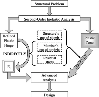
As shown earlier in the companion paper, inelastic analysis can have different approxima-tions and Chen [10] presented a summary of all the kinds of advanced analysis developed in recent years. A simplified block diagram in Fig. 1 illustrates the complete idea.
INDIRECTLY
Structural Problem
Second-Order Inelastic Analysis
Refined Plastic Hinge Plastic Zone Member out-of-straight Structure out-of-plumb Advanced Analysis Design DIR EC TL Y Et Residual stress INDIRECTLY Structural Problem
Second-Order Inelastic Analysis
Refined Plastic Hinge Plastic Zone Member’s out-of-straight Structure’s out-of-plumb Advanced Analysis Design DIR EC TL Y Et Residual stress INDIRECTLY Structural Problem
Second-Order Inelastic Analysis
Refined Plastic Hinge Plastic Zone Member out-of-straight Structure out-of-plumb Advanced Analysis Design DIR EC TL Y Et Residual stress INDIRECTLY Structural Problem
Second-Order Inelastic Analysis
Refined Plastic Hinge Plastic Zone Member’s out-of-straight Structure’s out-of-plumb Advanced Analysis Design DIR EC TL Y Et Residual stress
Figure 1 The advanced analysis concept.
First, the most known inelastic approximation is the refined plastic-hinge method (RPH) with their variations [10–12, 32], which has a respectable position in the scientific community. Here, methods provide the initial member’s out-of-straightness and residual stress indirectly in the analysis, because of the use of the tangent modulusEtto approximate the plasticity spread
effect, once yield begins. The Et modulus is determined and calibrated through standard
profiles profile experimental tests, where these imperfections are naturally included. Therefore, these methods implicitly provide both imperfections, and afterwards, the engineer needs only to incorporate the effect of the structure’s out-of-plumbness in the analysis [25].
approach to capture the plasticity spread with only one FE per member, even though there is not much cost in having more FEs per member, this latter now being the recommended procedure [10, 26].
Other methods that combine the refined plastic-hinge approach with improvements pointed out by the plastic zone technique, turned more versatile and oriented for the design office [4, 6, 25]. Barsan and Chiorean [6] refined their RPH method using Ramberg-Osgood curves to approximate P-M-Curvature functions developed by plastic zone analysis, but not considering the shift of the plastic center. Afterwards, they adjusted the axial deformation and curvature to previous forces gathered by a FE matrix, with the elastic terms corrected by the interaction diagram relationship [7].
Another general inelastic numerical approximation is the plastic zone technique. Besides being less popular and requiring more computing resources (memory, speed and process-time), it is more accurate and gives better information as to what is happening inside the member. For this reason, the use of this kind of approach defined some benchmark problems and specific criteria for the acceptance of some methods for advanced analysis [15, 30].
Some researchers [5, 27] used commercial packages like Abacus and Ansys to find 2D and 3D solutions for some benchmark problems using the plastic zone approach. On the other side, Foley and co-workers [18, 19] solved problems from hundreds of degrees of freedom through parallel processing and super-computers, with sub-structuring, condensation and vectorization techniques. Clarke [14, 29] developed some variation of the standard plastic zone technique for 3D analysis.
One of the main differences between the plastic zone approach and the other methods is that all imperfections are explicitly considered.
The plastic zone method adopted here is similar to that of Clarke’s [14], but more simplified and designed for the common personal computer. Moreover, as all information about the imperfections must be explicitly given, the engineer has to be careful to correctly include them in the finite element model.
Notwithstanding, the direct introduction of imperfect geometry and residual stress in the plastic zone method provides better information about their influence [15], as places where local buckling can happen, where high stress concentration appears, and where ductility demand can be present. More precisely, it also shows the equilibrium path from yielding to collapse or inelastic buckling. With this information, the engineer can avoid the combined effect of plasticity and buckling, which can appear along the member length together with other features (shear stress, welds, holes and other plane effects not covered here).
The three following sections illustrate the origin, the models, and imperfection incorpo-ration in the second-order inelastic analysis [2]. The study case explores a simple fixed-free imperfect column. The fifth section combines all the effects in a portal frame, which means application of the advanced analysis technique. Then, considerations about how to define geometric imperfections in a complex structural problem are made [2], justifying the final remarks.
2 MEMBER’S OUT-OF-STRAIGHTNESS
Because of exposure to cold after the rolling or welding process, structural bars usually are slightly deformed, which means they are not perfectly straight. Therefore, a bar has some initial curvature, even though the end sections remain straight, or are cut, parallel to each other. When these bars become the principal elements of a building (columns, beams and trusses), this type of geometric imperfection is incorporated in the steel construction.
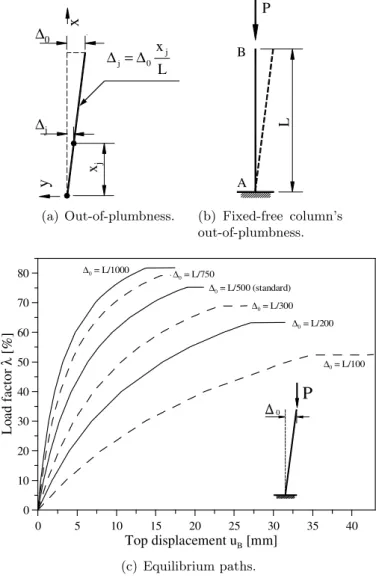
Researchers usually define an out-of-straight member as a member whose centerline turns to a sinusoidal half wave, with δ0 being the maximum amplitude at the middle length. When designing, this imperfection must be directed to the worst possible position in relation to the applied load. A standard defines the value of δ0 [1], and when this value is exceeded, some correction work should be done on the piece.
For computer programming, the initial out-of-straightness is modeled according to Fig. 2a, so that the entire finite element (FE) chain has its joints located at the sinusoidal arc (e.g. adopting δj for node j at position xj of one end of the member, where 0≤ xj ≤L, andL is
the length of the member). Because of the member’s axis representation, a small initial angle appears at the extreme nodes, independent of the boundary conditions, which means that the axis is no longer orthogonal to its support. For example, for a fixed column, this initial angle in the support node is fixed (it does not change throughout the analysis) and does not create initial forces.
To understand the effects of a member’s out-of-straightness, Fig. 2b presents a simple fixed-free column example that is studied throughout the first sections of this paper. The column is an 8 WF 31 standard section of ASTM A 36 steel (σy=25kN/cm2), with a length
ofL= 391.6 cm [22]. The goal is to define the largest load P that the column can bear, called the collapse load, with the presence of some imperfections (alone or combined), as a member’s out-of-straightness. Naturally, this collapse load Pc must obey: Pc≤Py≤Pe, where Py is the
crushing load and Pe is the elastic buckling load, i.e.:
Py=σyAg and (1a)
Pe=
π2
EIz
(kL)2 (1b)
where σy, E,k, Ag and Iz are the yield stress, Young modulus, equivalent length coefficient,
The axial load in curved members provides secondary moment amplification, related to stability, called the Pδ effect that reduces the strength of the column. Looking at the equi-librium paths represented in Fig. 2c, column top displacement uB is correlated to the load
factorλ(that varies from 0 to 100%), for some values ofδ0. As expected, whenδ0 grows from L/1500 to L/100, the load-factor at collapse decreases and the trajectory becomes longer and horizontal. As such, L/1000 is the design recommended design tolerance [12].
L /2 xj δ0 δj x y π δ = δ L x sin j 0 j L /2 xj δ0 δj x y L /2 xj δ0 δj x y π δ = δ L x sin j 0 j (a) Out-of-straightness. P L A B P L A B P L A B
(b) Fixed-free column’s out-of-straightness.
0 5 10 15 20 25 30 35 40
Top displacement uB [mm]
0 10 20 30 40 50 60 70 80 90 L o ad f ac to r λ [% ]
δ0 = L/1500
δ0 = L/100
δ0 = L/1000 (standard)
0
P
δ0 = L/750
δ0 = L/500
δ0 = L/300
δ0 = L/200
(c) Equilibrium paths.
3 STRUCTURE’S OUT-OF-PLUMBNESS
While the initial curvature comes from the manufacturing process, the structure’s out-of-plumbness is directly related to the erection or assembly of the steel frame. No matter how precise the concrete base and settlements are, it is quite impossible to provide vertical alignment for all the structural columns. Small differences always appear that require some adjustment on site, and this is the main cause of such an imperfection. This differences can be due to shape and length tolerances, clean space between holes and bolts, method and sequence of assembly, installing and tightening of bolts and anchors, and thermal effects of field welding (the welds tends to contract after the first strings).
For only one member, the computer implementation of this imperfection is very simple and similar to out-of-straightness, as it is a linear function represented in Fig. 3a, where xj is the
position of some nodej. The extreme value of the structure’s out-of-plumbness is ∆0, whose maximum standardized value is defined at L/500 [20].
Again, the small angle that appears in the support due to this initial imperfection is independent of the boundary condition.
This imperfection is very important for stability because it bonds to a well-known moment amplification behavior, called the P∆ effect. Figure 3b shows the same example treated in the section’s end and the equilibrium paths in Fig. 3c shed some light upon this effect. See the reduction on the collapse load when the structure’s out-of-plumbness increases. This influence is very critical.
It is worth mentioning that the P∆ Method, called notional loads [12], also approximates the instability effect through additional horizontal loads. Nevertheless, this strategy is quite different from what is done here, where the plasticity spread is evaluated step by step, which can anticipate the inelastic buckling, considering the actual axial force acting at the moment on every section, together with member strength degeneration. Usually the P∆ Method only produces the acting moments and the answers are usually overestimated.
4 RESIDUAL STRESS
All the steel construction substrate, such as standard sections, plates, and tubes, have some kind of residual stress born from unequal cooling of the parts, after the rolling, cutting and welding processes. Mechanical operations can also produce residual stress to cold-formed sections. Some other unstudied causes of residual stress are related to the manufacturing processes of drilling, welding and cutting. Therefore, it is possible to define residual stress as a natural consequence of every manufacturing or assembly task that involves local heating followed by unequal cooling.
Following Fig. 4a, as they are exposed to air, the section’s external parts cool first and contract. Later, when the still-hot parts of the section start to cool, they create tension stress, as contraction is inhibited. Figure 4b shows the compression stress in the section’s external parts, which is responsible for inhibiting contraction in the internal part.
How-xj
∆0
∆j
x
y
L xj 0 j=∆
∆
xj
∆0
∆j
x
y
L xj 0 j=∆
∆
(a) Out-of-plumbness.
P
L
A B
P
L
A B
(b) Fixed-free column’s out-of-plumbness.
0 5 10 15 20 25 30 35 40
Top displacement uB [mm]
0 10 20 30 40 50 60 70 80
L
o
a
d
f
ac
to
r
λ
[%
]
∆0 = L/1000
∆0 = L/100
∆0 = L/500 (standard)
0
P
∆0 = L/750
∆0 = L/300
∆0 = L/200
(c) Equilibrium paths.
Figure 3 Structure’s out-of-plumbness modeling and influence.
ever, this cleaning process seldom employs hammering or sand blasting to remove all the dust. This task can relieve some of the stress when coupled with normalization (heating to a temperature of 500 ○C, followed by room temperature cooling 20○C).
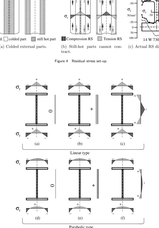
The residual stress (RS) distribution is self-equilibrated and the actual stress profile shows a different and complex shape, as the one reproduced in Fig. 4c [16]. There are several residual stress profile models, and some of them are in Fig. 5. Figures 5a,b,c represent the linear models and the parabolic models are in Figs. 5d,e,f. Figure 5b shows the Galambos and Ketter’s model [21], adopted by Kanchanalai [24], which is the basis of the AISC-LRFD [1] design procedure, also applied here in the examples. Figure 5c represents the model developed by ECCS [17], with some parabolic variation pictured in Fig. 5f.
i. flange ii. web i. flange ii. web
colded part still hot part Legend: colded part still hot part Legend:
(a) Colded external parts.
i. flange ii. web
σr
i. flange ii. web
σr
Compression RS Tension RS Compression RS Tension RS
(b) Still-hot parts cannot con-tract.
RS
σr
σr N/mm2
14 W 730 A36
100 50 0 -50
-50 0 50 100
-50 0 50 100
RS
σr
σr N/mm2
14 W 730 A36
100 50 0 -50
-50 0 50 100
-50 0 50 100
(c) Actual RS diagram.
Figure 4 Residual stress set-up.
(d) (e) (f)
Parabolic type
(a) (b) (c)
Linear type
σ
rσ
rσ
rσ
r0
0
+
+
(d) (e) (f)
Parabolic type
(a) (b) (c)
Linear type
σ
rσ
rσ
rσ
r0
0
+
+
stress. Figures 6a,c show the welding of hot-rolled plates, while Figs. 6b,d portray the heat-cut plates. High-tension stress (near yielding stressσy) appears close to the welding bath, inducing
compression stress on the extremities due to the welding. In the case of hot-cut plates, see the remaining tension stress at the flange tips. The present paper, however, focuses on rolled shapes only.
σr
σr
σr
σr
Before welding
After welding
σr
σr
σr
σr
σr
σr
σr
σr
σr
σr
σr
σr
Before welding
After welding
(a) Rolled plates. (b) Hot-cut plates. (c) Welded rolled plates. (d) Welded hot-cut plates.
Figure 6 Residual stress diagrams of built-up sections.
The beam-column problem, already studied in the companion paper, brings some light on the residual stress effects, as illustrated in Fig. 7. There is some reduction of the beam-column capacity for all the selected slenderness (L/rz = 60, 80, 100) due to Galambos and Ketter’s
residual stress model [21]. The present work’s findings follow those from the BCIN program [11, 14].
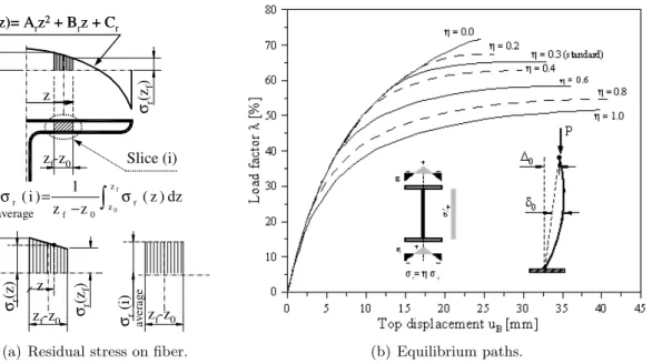
The computational modeling of this imperfection is made here defining an average stress value with no deformation, for every fiber, in all slices of the model. This average stress is determined directly in the linear diagrams, while in the parabolic and other nonlinear models, average integration on the slice produces the fiber’s residual stress (see Fig. 8a). This figure shows thatσr(z)is the adopted approximation for the residual stress’s parabolic function (e.g.,
Arz2+Brz+Cr) or linear function, where z defines the position in the slice (0≤z≤zf),zf is
the length of slice that is parallel to the integration axis, and (i) is the ith slice [3].
The self-equilibrating residual stress produces no resultant force. However, yielding appears quickly where the working stress adds to the residual ones; or appears late in those slices where these stresses have an unequal sign. Further, the nonlinear equilibrium paths also become less abrupt and a little longer.
The maximum residual stress in the linear model of Fig. 5b occurs at the flange tip and can be represented by equationσr=ησy, with 0≤η≤1, preferably with the ηparameter equal
to 0.3 [21]. Figure 8b illustrates the equilibrium paths of the fixed-free column studied in previous sections, when this residual stress’s linear model is adopted with a variable maximum parameter η and a worst geometric imperfection situation (see next section). This figure can highlight the commentary on the nonlinear paths stated before. See that the non-residual stress’s equilibrium path has the highest collapse load and a smaller top column displacement uB. Naturally, the less steep and most extended path is the one withη=1, which produced the
worst answer for the design. This last comment pointed out the need for an advanced direct analysis, mainly when dealing with built-up sections, since they have the highest residual stresses (η near to 1) captured in experimental work [20].
σr (z0 ) σr (zf ) σr (z0 ) σr (zf ) σr (z ) σr (i ) z
zf-z0
zf-z0 zf-z0
z dz ) z ( z z 1 ) i ( f 0 z z r 0 f
r = − σ
σ a v e ra g e
σr(z)= Arz2+ Brz + Cr
Slice (i) average σr (z0 ) σr (zf ) σr (z0 ) σr (zf ) σr (z ) σr (i ) z
zf-z0
zf-z0 zf-z0
z dz ) z ( z z 1 ) i ( f 0 z z r 0 f
r = − σ
σ a v e ra g e
σr(z)= Arz2+ Brz + Cr
Slice (i)
average
(a) Residual stress on fiber. (b) Equilibrium paths.
5 ADVANCED ANALYSIS CONCEPT
By considering geometric imperfections (related to stability effects P∆ and Pδ) and physical imperfections (related to material inelastic behavior and residual stress), the numerical com-putational models can provide answers very close to those in standards, which are generally based on the consolidated findings of many years. As these numerical answers follow the main design requirements, there is no meaning or need to perform additional member strength checks. That is why this analysis is called “advanced” [12]: a step toward the designing job.
Firstly, the combined effect of the two studied initial geometric imperfections deserves spe-cial attention. The initial curvature must be applied first and then the out-of-plumb effect is added in such a way that the amplitude δ0 is still maximum at the member’s middle, as represented in Fig. 9a. This order recognizes that out-of-straightness is born during manufac-turing, while out-of-plumbness appears in the assembly process. Figure 9b shows a different model when the reverse order is adopted (δ0 is not in the middle because it turns oblique to out-of-plumb angle ∆0/L [22]).
δ0
∆0
∆0
δ0
∆0
∆0
δ0 δ0
+
=
+
=
δ0
∆0
∆0
δ0
∆0
∆0
δ0 δ0
+
=
+
=
(a) Out-of-straightness and out-of-plumbness. (b) Reverse order (not recommended).
Figure 9 Combination of initial geometric imperfections.
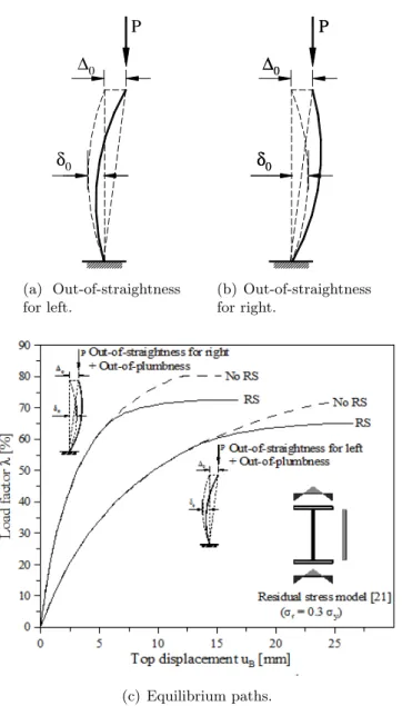
Now, to understand the advanced analysis concept, it is used the same fixed-free column problem, beginning with only imperfect geometric models (e.g. ignoring initially RS). Figures 10a,b illustrate two possible configurations through the combination of out-of-straight (OS, for left and right) and out-of-plumb (OP) imperfections. At first, it would seem that Fig. 10b is the worst situation, but as can be seen in Fig. 10c, the equilibrium paths of both configurations prove that the worst and governing one is the first imperfect model (OS for left).
After determining the worst imperfect geometric configuration, we introduce the residual stress effect. Figure 10c also shows that this effect reduces both imperfect fixed-free column collapse loads. Therefore, the worst imperfect geometry (Fig. 10a; OS for left, OP and RS) will lead to the governing advanced analysis answer.
Table 1 shows that the collapse load for the just-described conditions, whether or not residual stress (RS) is included, and even for notional load (horizontal forceHat the column top similar to an OP ofL/500). For comparison, we used the answers presented in Hajjaret al. [22]. Good agreement between the results validates this paper inelastic formulation for designing a single member. Thence, the design load P for this problem is λlowPy = 0.651×1472.5 =
resistance must be multiplied by 0.9 and must also be greater then the factored load (e.g., Pf act≤0.9×958=862 kN).
∆0
δ0
P
∆0
δ0 ∆0
δ0
P
(a) Out-of-straightness for left.
∆0
δ0
P
∆0
δ0
P
∆0
δ0
P
(b) Out-of-straightness for right.
(c) Equilibrium paths.
Figure 10 Advanced analysis of fixed-free column.
The Vogel’s portal [31] presented in the companion paper, included pre-defined geometric and residual stress imperfections, and showed good theoretical agreement. This also validates the present formulation for the advanced analysis of a set of members.
Table 1 Collapse load factorλof fixed-free column [22].
Case Geometric Imperfection Models (1)
Figure (2)
λ: Hajjar et al. [22] λ: Present work (3)
No RS With RS No RS With RS
1 No imperfection - 1.000 - 0.7361 (3)
0.5972(3)
2 OP 3b 0.750 0.681 0.7512 0.6839
3 OS (L or R) 2b 0.823 0.727 0.8239 0.7279
4 OP + OS L 10a 0.712 0.650 0.7148 0.6516
5 OP + OS R 10b 0.801 0.723 0.8019 0.7258
Notes: 1. Abbreviations: OP (out-of-plumbness), OS (out-of-straightness), RS (residual stress), L (left) and R (right); 2. Figures related to imperfect geometry; 3. LoadP=λF (the authors
usedF = 2000 kN;Py= 1472.5 kN).
complex structural problems.
6 STEEL PORTAL FRAME STUDY
It took little effort to explicitly include the initial geometric imperfections for studying the single member behavior in the previous sections. The foregoing portal frame study presents its data in Fig. 11. For this portal frame with three members, the question arises as to how to incorporate standard initial out-of-straightness and out-of-plumbness to capture the worst condition.
Data:
P = λPy 0 λ 100 % H = 0.5 Hy
steel: ASTM A 36 E = 20000 kN/cm2
σy= 25 kN/cm2 Section: 8 WF 31
δ0= A / 1000 = 0.36 cm
∆0= A / 500 = 0.71 cm Galambos & Ketter RS with σr= 0.3 σy [21]
P P P P
A
=
3
3
5
.6
c
m
A
=
3
3
5
.6
c
m
H H
B = 533.4 cm B = 533.4 cm
δ0
δ0
∆0= 0.71 cm
= 0.36 cm
A D
C B
Figure 11 Steel portal frame.
Figure 12 shows four different geometric configurations incorporating only the columns’ out-of-straightness. The worst condition is the Fig. 12d case.
δ
0δ
0δ
0δ
0P
P
P
P
H
H
δ
0δ
0δ
0δ
0P
P
P
P
H
H
(a) Left-left. (b) Left-right.
δ
0δ
0δ
0δ
0P
P
P
P
H
H
δ
0δ
0δ
0δ
0P
P
P
P
H
H
(c) Right-left. (d) Right-right.
Figure 12 Portal frame with members’ out-of-straightness.
final frame collapse and worst imperfect geometry design.
P
P
P
P
H
H
∆0
∆0
∆0
∆0
P
P
P
P
H
H
∆0
∆0
∆0
∆0
(a) Left-left. (b) Left-right.
P
P
P
P
H
H
∆0
0
∆0
∆0
∆0
P
P
P
P
H
H
∆0
0
∆0
∆0
∆0
(c) Right-left. (d) Right-right.
Figure 13 Portal frame’s out-of-plumbness.
Figure 14 illustrates twelve possible different frame configurations through a combination of out-of-straight and out-of-plumb imperfections. The worst condition is in Fig.14a, as shown in Table 2.
P P P P P P P
P P P P P P P
P P P P P P P
P
P
P
H H H H
H H H H
H H H H
∆0 ∆0 ∆0 ∆0 ∆0 ∆0 ∆0 ∆0
∆0 ∆0 ∆0 ∆0 ∆0 ∆0 ∆0 ∆0
∆0 ∆0 ∆0 ∆0 ∆0 ∆0 ∆0 ∆0
δ0 δ0 δ0 δ0 δ0 δ0 δ0 δ0
δ0 δ
0 δ0 δ0 δ0 δ
0 δ0 δ0
δ0 δ0 δ0 δ0 δ0 δ0 δ0 δ0
(a) (b) (c) (d)
(e) (f) (g) (h)
(i) (j) (k) (l)
P P P P P P P
P P P P P P P
P P P P P P P
P
P
P
H H H H
H H H H
H H H H
∆0 ∆0 ∆0 ∆0 ∆0 ∆0 ∆0 ∆0
∆0 ∆0 ∆0 ∆0 ∆0 ∆0 ∆0 ∆0
∆0 ∆0 ∆0 ∆0 ∆0 ∆0 ∆0 ∆0
δ0 δ0 δ0 δ0 δ0 δ0 δ0 δ0
δ0 δ
0 δ0 δ0 δ0 δ
0 δ0 δ0
δ0 δ0 δ0 δ0 δ0 δ0 δ0 δ0
(a) (b) (c) (d)
(e) (f) (g) (h)
(i) (j) (k) (l)
Figure 14 Combined initial geometrical imperfections of steel portal frame. Table 2 Combination of initial geometric imperfections of steel portal frame.
Load factor H=βHHy
(2)
OP + OS(1)
[%] a: b: c: d: e: f:
λy (3)
βH = 0.0 91.4 89.8 97.1 95.8 89.5 97.1
βH = +0.5 55.8 56.1 59.2 59.2 54.9 61.5
λcol (
4) βH = 0.0 92.7 93.4 97.6 97.4 93.5 97.6
βH = +0.5 64.5 64.9 67.5 68.0 65.0 68.5
Load factor
H=βHHy
OP + OS(1)
[%] g: h: i: j: k: l:
λy (3)
βH = 0.0 95.9 92.4 97.1 95.9 95.8 97.1
βH = +0.5 58.1 57.9 59.0 59.1 57.9 61.3
λcol (
4) βH = 0.0 97.3 93.8 97.5 97.4 97.3 97.5
βH = +0.5 68.0 65.4 67.4 67.8 67.9 68.3
Notes: 1. Abbreviations: OP (out-of-plumbness) and OS (out-of-straightness); 2. Two loading cases: with H (βH = 0.5) and noH (βH = 0), whereHy=2Mp/L,Mp is the section plastic
moment andLis the column length; 3. λy: yield start; and 4. λcol: collapse load factor.
(RS) following Galambos and Ketter’s approximation [21]. Table 3 presents all related collapse loads, including or not the horizontal load H, and with and without the residual stress effect. See that the loadP =0.633×1472.5=932 kN is the minimum collapse load forH=0.5Hy=35
kN; andP =0.903×1472.5=1330 kN when no horizontal forceH occurs.
Table 3 Advanced analysis of steel portal frame.
(a) With horizontal loadH (βH=0.5)
Case Geometry case (1) Fig. (2) Load factor [%] no RS(
1)
Load factor [%] with RS (1)
λy (
3) λ
col (
4)
λy (
3)
λcol (
4)
1 No imperfection 11a 60.2 68.0 35.5 66.4
2 OS 12a 59.1 67.4 34.8 66.0
3 OP 13d 56.9 65.0 33.6 63.6
4 OS + OP combined 14a 55.8 64.5 33.0 63.3
(b) No horizontal loadH (βH=0; only vertical 2P load)
Case Geometry case (1)
Fig. (2) Load factor [%] no RS(
1) Load factor [%] with RS (1)
λy (3) λcol (4) λy (
3) λ
col (4)
1 No imperfection 11a 100.0 72.5 97.9
2 OS 12b 95.9 97.3 69.5 96.1
3 OP 13d 93.1 94.2 67.8 91.1
4 OS + OP combined 14a 91.4 92.7 66.5 90.3
Notes: 1. Abbreviations: OP (out-of-plumbness), OS (out-of-straightness) and RS (residual stress); 2. Figures related to imperfect geometry; 3. λy: yield start; and 4. λcol: collapse load
factor.
P =1197 kN only when factored vertical loads occur. Additionally, there is no need to perform other member’s checks for in-plane strength and stability.
While a single fixed-free column had only four different combined configurations, the por-tal frame needed twenty different models. After these analyses, one can wonder how many geometrically imperfect combinations are necessary to test a complex structural problem in order to figure out the worst one, so it can be applied to the advanced analysis concept, since residual stress can be included afterwards. The next paragraphs will discuss this subject.
Take the worst fixed-free column initial geometrically imperfect configuration in Fig. 10 and the deformed geometry of the portal frame at collapse load, as represented in Fig. 15a (fixed-free column together with a hinged stiff beam and another similar column). Then observing the corresponding deformed configuration at collapse and comparing it with the portal frame’s worst initial geometric imperfection and its behavior at collapse (Figs. 14a and 15b), it seems that the only logical answer to explain how these imperfect configurations are more critical than others, comes from its own deformed shape at collapse.
Still, comparing all the deformed imperfect frame configurations at collapse load, it seems that these structural systems would have the same final deformed shape (the forces applied to the systems are the same in all cases). However, some geometrically imperfect frames require more deformation energy to reach the collapse configuration than do others, which is explained by the fact that some imperfections are contrary to the final frame collapse shape, while others contribute to a more easily collapsible structure.
P Infinitely P
Rigid Beam
P Infinitely P
Rigid Beam
P Infinitely P
Rigid Beam
(a) Fixed-free column mounted as a frame.
P P
H
P P
H
P P
H
(b) Portal frame study: worst initial geometrical model.
Figure 15 Collapsed configuration using advanced analysis.
configuration.
After studying this question, it is possible to conclude: “the most critical initially imperfect
geometry (that produces the least collapse load-factor for some loading cases of the structure),
is the closest to the final collapse configuration, since it requires the least deformation energy
to go from the unload state to the final collapse situation.” This statement is only valid when
there is no conflict between the load’s action (P∆, Pδ, etc) and the collapse configuration [2], which means there is a point of equilibrium divergence [16].
The basis of this idea is the work of Chwalla [13], who proposed a procedure to obtain the deformed shape of buckled columns by determining the forces acting on the system. There-fore, if the curves that describe the column’s state at collapse are the same, the imperfect configuration that needs lower loads to reach collapse is that which has its shape nearest to the collapse shape. Chwalla’s work included any type of column.
The proof of this conclusion is based on a same-frame analysis, where the imperfect geom-etry is opposite to the critical one (see Fig. 16a). The final collapse shape is in Fig. 16b and is similar to the critical initial geometric configuration in Fig. 15b, except that the collapse load-factor is the highest one (λ = 71.8%). Therefore, the opposite configuration needs the largest deformation energy to reach its collapse.
Considering these comments, an engineer can first make a structural second-order inelastic analysis to obtain the final collapse configuration for some loading cases. Afterwards, the structure structure’s final deformed shape is used to model the required initial geometric imperfection in the advanced analysis (e.g., the initially imperfect geometry should follow the collapse configuration). Finally, the residual stress is introduced into the solution process, and the advanced direct analysis will define the collapse load-factor for this problem [3].
δ0
δ0
P P
H
∆0
∆0
δ0
δ0
P P
H
∆0
∆0
δ0
δ0
P P
H
∆0
∆0
(a) Opposite of the worst geometrical config-uration.
P P
H
P P
H
P P
H
(b) Correspondent collapsing deformed geome-try.
Figure 16 Effect of opposite of the worst initial geometrical configuration model.
7 FINAL REMARKS
The advanced analysis approach (plastic-zone method or even refined plastic-hinge method) is not yet effectively adopted in design offices but as computer capacities increase, this condition is changing and becoming more feasible. As such, there is a future for the use of this approach. By adopting models with imperfect geometry and residual stress, a deep insight of struc-tural behavior can be obtained because it precisely portrays the states of ultimate strength and stability, allowing the engineer to avoid or to reduce complementary member checks. To un-derstand and apply this design concept, the engineer must precisely define the initial imperfect geometry; the authors have provided recommendations for this task in this paper.
As already mentioned, the importance of initial imperfect geometry is connected to a stability problem, while residual stress both makes yielding begin earlier than foreseen and the plastic path widens inducing plastic inelastic buckling.
Moreover, even though plastic-zone analysis spends a lot of processing time and requires memory resources, the knowledge of plasticity spread along the members describes the whole picture of structural behavior. With this tool, the engineer can provide a safe structural design that avoids local buckling and high stress concentration. The authors’ future research will introduce semi-rigid connection behavior [28] into the models to study its influence on the proposed recommendation.
Acknowledgments The authors are grateful for the financial support from the Brazilian
References
[1] AISC LRFD. Load and resistance factor design specification for structural steel buildings. Chicago, Illinois, USA, 2nd edition, 1993.
[2] A.R. Alvarenga. Main aspects in plastic-zone advanced analysis of steel portal frames. Master’s thesis, Civil Engi-neering Program, EM/UFOP, Ouro Preto, MG, Brazil, 2005. In Portuguese.
[3] A.R. Alvarenga and R.A.M. Silveira. Considerations on advanced analysis of steel portal frames. In Proceedings of ECCM III European Conference on Computational Mechanics – Solids, Structures and Coupled Problems in Engineering, page 2119, Lisbon, Portugal, 2006.
[4] M.R. Attalla, G.G. Deierlein, and W. McGuire. Spread of plasticity: a quasi-plastic hinge approach. Journal of Structural Engineering ASCE, 120(8):2451–2473, 1994.
[5] P. Avery and M. Mahendran. Distributed plasticity analysis of steel frame structures comprising non-compact sections.Engineering Structures, 22:901–919, 2000.
[6] G.M. Barsan and C.G. Chiorean. Computer program for large deflection elasto-plastic analysis of semi-rigid steel frameworks.Computer and Structures, 72:699–711, 1999.
[7] G.M. Barsan and C.G. Chiorean. Influence of residual stress on the carrying capacity of steel framed structures. numerical investigation. In D. Dubina and M. Ivany, editors,Stability and Ductility Steel Structures, SDSS’99, pages 317–324. Elsevier Science Publishing, 2000.
[8] S.L. Chan and P.P.T. Chui. A generalized design-based elastoplastic analysis of steel frames by section assemblage concept.Engineering Structures, 19(8):628–636, 1997.
[9] S.L. Chan and H. Zhou. Non-linear integrated design and analysis of skeletal structures by 1 element per member.
Engineering Structures, 22:246–257, 2000.
[10] W.F. Chen. Structural stability: from theory to practice. Engineering Structures, 22:116–122, 2000.
[11] W.F. Chen, Y. Goto, and J.Y.R. Liew.Stability design of semi-rigid frames. John Willey and Sons, New York, 1996. [12] W.F. Chen and D.W. White. Plastic hinge based methods for advanced analysis and design of steel frames – An
assessment of the state-of-the-art. SSRC, Bethlehem, 1993.
[13] E. Chwalla. Theorie des aussermmittig gedruckten stabes aus baustahl. Stahlbau, 7:10–11, 1934.
[14] M.J. Clarke. In W.F. Chen and S. Toma, editors,Advanced analysis of steel frames: theory, software and applications, Boca Raton, 1994. CRC Press.
[15] M.J. Clarke, R.Q. Bridge, G.J. Hancock, and N.S. Trahair. Advanced analysis on steel building frames. Journal of Constructional Steel Research, 23:1–29, 1992.
[16] ECCS.Manual on Stability of Steel Structures, 1976.
[17] ECCS. Ultimate limit states calculations of sway frame with rigid joints. Technical report, Technical working group 8.2, Publication 33, European Convention for Constructional Steelwork, Brussels, 1984.
[18] C.M. Foley. Advanced analysis of steel frames using parallel processing and vectorization.Computer-aided Civil and Infra. Eng., 16:305–325, 2001.
[19] C.M. Foley and D. Schinler. Automated design of steel frames using advanced analysis and object-oriented evolu-tionary computation. Journal of Structural Engineering ASCE, 129(5):648–660, 2003.
[20] T.V. Galambos. Structural members and frames. Technical report, Dept. Civil Engineering – Univ. Minnesota, Mineapolis, 1982.
[21] T.V. Galambos and R.L. Ketter. Columns under combined bending and thrust. Transations ASCE, 126(1):1–25, 1961.
[22] J.F. Hajjar. Effective length and notional load approaches for assessing frame stability: Implications for american steel design. Technical report, Task Committee on Effective Length of the Technical Committee on Load and Resistance Factor Design of the Technical Division of the Structural Engineering Institute of the American Society of Civil Engineers, Reston, Va., 1997.
[24] T. Kanchanalai. The design and behavior of beam-column in unbraced steel frames. Technical Report AISI Project 189 Rep. 2, Univ. Texas, Civil Eng. Structural Research Lab, Austin, Texas, USA, 1977.
[25] S.E. Kim and W.F. Chen. Practical advanced analysis for unbraced steel frame design. Journal of Structural Engineering ASCE, 122(11):1259–1265, 1996.
[26] S.E. Kim and W.F. Chen. A sensivity study on number of elements in refined plastic-hinge analysis. Computers & Structures, 66(5):665–673, 1998.
[27] S.E. Kim and D.H. Lee. Second-order distributed plasticity analysis of space steel frames. Engineering Structures, 24:735–744, 2002.
[28] L. Pinheiro and R.A.M. Silveira. Computational procedures for nonlinear analysis of frames with semi-rigid connec-tions. Latin American Journal of Solids and Structures, 2:339–367, 2005.
[29] L.H. Teh and M.J. Clarke. Plastic-zone analysis of 3d steel frames using beam elements. Journal of Structural Engineering ASCE, 125(11):1328–1337, 1999.
[30] S. Toma and W.F. Chen. Calibration frames for second-order analysis in japan. Journal of Constructional Steel Research, 28:51–77, 1994.
[31] U. Vogel. Calibrating frames.Stahlbau, 10:295–301, 1985.

![Figure 7 Residual stress effect on Galambos and Ketters beam-column [21].](https://thumb-eu.123doks.com/thumbv2/123dok_br/15701200.629102/9.892.264.576.648.961/figure-residual-stress-effect-galambos-ketters-beam-column.webp)