doi: 10.1590/0101-7438.2015.035.02.0377
A MODEL SELECTION PROCEDURE IN MIXTURE-PROCESS EXPERIMENTS FOR INDUSTRIAL PROCESS OPTIMIZATION
M´arcio Nascimento de Souza Le˜ao
1, Antonio Fernando de Castro Vieira
2and Luiz Henrique Abreu Dal Bello
3*Received September 19, 2012 / Accepted September 27, 2014
ABSTRACT.We present a model selection procedure for use in Mixture and Mixture-Process Experiments. Certain combinations of restrictions on the proportions of the mixture components can result in a very constrained experimental region. This results in collinearity among the covariates of the model, which can make it difficult to fit the model using the traditional method based on the significance of the coefficients. For this reason, a model selection methodology based on information criteria will be proposed for process optimization. Two examples are presented to illustrate this model selection procedure.
Keywords: mixture experiments, process optimization, information criterion, multicollinearity.
1 INTRODUCTION
Formulations obtained from Mixture Experiments (ME) are commonly found in the chemical, pharmaceutical, and food industries, as well as in other industrial segments. In those experiments, the decision variables are the proportions of the components in a mixture and the response is a variable that characterizes the quality of the product, assumed as a function of component propor-tion. In these experiments, the sum of component proportions is always equal to one. In certain industrial processes, there may be other variables, in addition to the mixture components, that affect the characteristics of the process and must be included in the experiment as factorial de-signs. Such experiments are called Mixture-Process Experiments (MPEs). Therefore, we intend to determine not only the optimal proportions of the mixture components but also the optimal levels of the process variables.
*Corresponding author.
1Department of Industrial Engineering, Pontifical Catholic University of Rio de Janeiro (PUC-Rio), Rio de Janeiro, RJ, Brazil. E-mail: [email protected]
2Department of Industrial Engineering, Pontifical Catholic University of Rio de Janeiro (PUC-Rio), Rio de Janeiro, RJ, Brazil. E-mail: [email protected]
In MEs, it might be necessary to limit the proportion of one or more components that, for tech-nical or practical reasons, cannot be present in all possible proportions. Those limitations of the components, which are very common in industrial cases, may be upper, lower, or a combination of both. Certain combinations of limitations on the proportions of the components may result in a very limited experimental region, which results in collinearity among the covariates of the model, making it difficult to fit the model using the traditional method based on the significance of the coefficients. Consequently, a model selection methodology based on information criteria will be proposed. In order to illustrate this methodology, two examples are used. MatlabR routines were
then written for the model selection and the process optimization.
Cornell (2002) is the main reference on ME, being the Chapter 7 dedicated to MPE cases. In it, a comprehensive and detailed exposition can be found. Myers & Montgomery (2002) dedicate Chapters 12 and 13 to ME and MPE, thus comprising a good introduction to the topic. Piepel (2004) summarizes a survey related to mixture experiments for a period of 50 years, ranging from 1955 to 2004. Prescott et al. (2002) propose a quadratic model as an alternative to the models traditionally used in ME (Scheffe models). Cornell (2000), Cornell (2002, Chapter 6), Cornell & Gorman (2003) and Khuri (2005) carried out comparative studies between models that they named as slack-variable models and Scheff´e models. Piepel (2007) compares the CSLM (Com-ponent Slope Linear Model) with the SLM (Scheff´e Linear Model) and the CLM (Cox Linear Model). They conclude that the models SLM, CLM and CSLM are mathematically equivalent and provide the same statistics for a given ME. The differences lie in the interpretations of their coefficients. Dal Bello & Vieira (2011b) present a tutorial on mixture-process experiments.
Goos & Donev (2006) describe an algorithm to plan experiments in blocks involving mixtures. They show that, for restricted and unrestricted experimental regions, the resulting design of ex-periments is statistically more efficient than the options of exex-periments in blocks presented in the literature. Goos & Donev (2007) describe an algorithm to plan split-plot experiments in cases involving mixture and process variables. They use an optimization criterion for the choice of ex-perimental points and show that it is preferable to spread the replications all over the experiment region, instead of concentrating them in central points.
Kowalski et al. (2002), Prescott (2004) and Sahni et al. (2009) analyzed the MPE modeling. Goldfarb et al. (2004a) propose the use of a plot method (variance dispersion plot) for MPE planning. The variance dispersion plot presents a visual way of assessing the variance properties of an MPE within the joint mixture and process area. That information may be used to select experiments with an acceptable variance profile.
Dal Bello (2010) Dal Bello & Vieira (2011a) present a methodology close to the spirit of this article.
A brief introduction to ME and MPE is presented in Sections 2 and 3. In Section 4, the infor-mation criteria used in this work are described and the models chosen according to those criteria are presented. In Section 5, we present a model selection methodology with two examples, and we apply this methodology in two other examples. The conclusions are in Section 6.
2 MIXTURE EXPERIMENTS
Considerxi, the variables that represent the proportions of theq mixture components. Then: q
i=1
xi =1; xi ≥0; i =1, . . . ,q (1)
In many MEs there are limitations on the component proportions, making the experimental space a sub-region of the original space. Therefore, upper and/or lower limits on the proportions are established, and are represented as follows:
0≤Li ≤xi ≤Ui ≤1; i =1, . . . ,q (2)
whereLi is the lower limit andUi is the upper limit of the component proportioni.
When the upper and lower limits on the proportions of one mixture are established, the experi-mental region is reduced to a sub-region of the original region. In these cases, the coordinates of the sub-regions may be redefined in terms of “pseudo”-components.
The models which are traditionally used in MEs are Scheff´e’s canonical polynomials (Scheff´e, 1958). Scheff´e’s cubic model is as follows:
C(β,x) =
q
i=1
βixi+
q
i<j
βi jxixj +
q
i<j<k
βi j kxixjxk
+
q
i<j
βi−jxixj(xi−xj)
(3)
where theβs are the model’s parameter coefficients. Note that this model does not have the intercept, as it is eliminated by a simplification originating from the basic limitation presented in Eq. (1).
3 MIXTURE-PROCESS EXPERIMENTS
An adequate model for r process variablesz1,z2, . . . ,zr involving second-order terms is:
Q(δ,z)=δ0+ r
l=1
δlzl+ r
l=1
δllzl2+
r
l<m
where theδs are the model’s parameter coefficients for process variables. The experiment for the process variables may be a factorial design with two or more levels. In order to include terms with the variablez2j in the model, an experiment with at least three levels of each process variable and a total number of points sufficient to fit and test the model is required. In order to fit a model without the variablez2j, considering only the main effects of the process variables and the interactions among them, only two levels of each variable are necessary.
We use the form of the simultaneous additive and multiplicative combined model, which includes Scheff´e’s cubic model for the mixture and the reduced quadratic model, considering only the main effects of the process variables and the interactions among them:
C(γ , δ,x,z)=
q
i=1
yilxi+
q
i<j
γi jl xixj+
q
i<j<k
γi j kl xixjxk
+
q
i<j
γil−jxixj(xi −xj)+ r
l=1
δlzl+
r
l<m
δlmzlzm
+
r
l=1 ⎡ ⎢ ⎢ ⎢ ⎢ ⎢ ⎣ q
i=1
γilxi +
q
i<j
γi jlxixj +
q
i<j<k
γi j kl xixjxk
+
q
i<j
γil−jxixj(xi−xj)
⎤ ⎥ ⎥ ⎥ ⎥ ⎥ ⎦ zl + r
l<1 ⎡ ⎢ ⎢ ⎢ ⎢ ⎢ ⎣ q
i=1
γilxi +
q
i<j
γi jlxixj +
q
i<j<k
γi j kl xixjxk
+
q
i<j
γil−jxixj(xi−xj)
⎤ ⎥ ⎥ ⎥ ⎥ ⎥ ⎦
zlzm
(5)
where theγs are the parameters for the mixture’s combined model including process variables and theδs are the parameters for the process variables. The lower indexes ofγ refer to mixture variables, whereas the upper ones refer to process variables. The lower indexes ofδ refer to process variables.
4 INFORMATION CRITERIA AND MODEL SELECTION
An information criterion that has been widely used in model selection is Akaike’s criterion (AI C) (Akaike, 1973).
AI C = −2
n
i=1
lnL(µˆi,yi)+2p (6)
is a distance between the true model and the candidate model. Burnham & Anderson (2002) recommend the use ofAI C only whenn/p≥40. Considering a case of responses with normal distribution, theAI C expression may be simplified to give the following:
AI C =nln(σˆ2p)+2(p+1) (7)
ˆ
φ2p=
n
i=1(yi− ˆφi)2
n (8)
whereσˆp2is the maximum likelihood estimator of the error variance.
Considering responses with normal distribution and small samples(n/p<40), Hurvich & Tsai (1989) developed the AICc criterion:
AI Cc =AI C+
2(p+1)(p+2)
n−p−2 (9)
Burnham & Anderson (2002) recommend the calculation ofAI C differences between the can-didate models and the model with the lowestAI Ccvalue(AI Cc min).
i = AI Cc i−AI Cc min (10)
The calculation methodology for AI C differences may also be used for AI Cc differences. i values can be interpreted easily and allow a quick comparison of candidate models. The higher thei, the less likely it is that the fitted model is the best model according to Kullback-Leibler distance. Burnham & Anderson (2002) affirm that models withi > 10 may be omitted in future considerations and models withi between 0 and 2 may be regarded as non-different. The calculation of AI Cc differences is used in the proposed methodology for model selection which will be used in Section 5.
5 PROPOSED METHODOLOGY
In the first stage of this methodology we use the full Scheff´e’s canonical polynomials for a ME and a combined model for a full MPE. Thus, we obtain all the candidate terms for the model under study. Then, we use theAI Cc criterion to select the model with the lowestAI Cc according to the number of parameters. Afterwards, we calculate theAI Ccdifferences between the candidate models and the model that has the lowest AICc and we select the non-different models.
Analyzing the non-different models, we choose the model, now named the Base Model, which has the lowest mean-squared error (MSE) and prediction error sum of squares (PRESS).
the candidate terms (terms of the Base Model and Equivalent Terms), we use the AI Cccriterion again in order to select the model with the lowest AI Cc. Afterwards, we calculate the AI Cc differences between the candidate models and model that has the lowestAI Ccand we select the non-different models.
Analyzing the non-different models, we choose the model with the lowest PRESS and MSE as the Final Model. The proposed methodology is illustrated through two examples.
5.1 Example 1
The problem of Example 1 was presented by Myers & Montgomery (2002). An adhesive is being formulated for use in an aerospace application. The adhesive consists of a resinx1and two crosslinkers,x2andx3. The mixture constraints for these variables arex1+x2+x3 =1; 0.70≤xi ≤0.90; 0.05≤x2≤0.10; and 0.05≤x2≤0.20.
The adhesive is applied to the components and then the entire assembly is cured for 12 h at controlled temperature and humidity. The temperature z1and relative humidityz2are process variables that can be controlled by the experimenter. The ranges of theses process variables that experimenters think are appropriate are 40◦F ≤temperature≤100◦F and 15%≤ relative hu-midity≤ 85%. The response variable of interest is the pulloff force required to separate the components after curing. It should exceed 40 pounds.
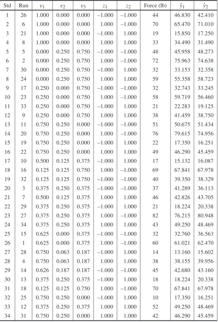
The authors use L-pseudocomponents according to the relationvi = x1i−−LL1; i = 1,2, . . . ,q, whereL = qi=1Liand Table 1 presents the experiment.
Where
ˆ
y1: Response obtained by Myers & Montgomery (2002) model.
ˆ
y2: Response obtained by Final Model 1 in this article.
The model selected by Myers & Montgomery (2002) presented PRESS, MSE and AI Cc equal to 903.20, 15.45 and 122.57, respectively, and is shown in Eq. (11).
ˆ
y = 40.66v1+71.95v2+46.16v3−30.58v1v3+9.32v1z1
−15.49v1z2+29.92v2z1−20.18v2z2+7.43v3z1
−4.41v3z2+19.39v1v3z1−2.60v3z1z2
(11)
5.1.1 Model Selection Methodology
All the candidate terms for the MPE are the terms in Eq. (5). The model selected according to theAI Cccriterion was the following:
ˆ
y = 40.36v1+67.32v2+35.09v3+11.79z1−16.19z2+11.25v3z2
−3.53v1z1z2−106.74v2v3(v2−v3)+172.09v1v2v3z1
−45.36v1v2z1z2+138.49v1v2z1z2(v1−v2)
(12)
A MatlabR routine was then written for the calculation and storage ofAI C
Table 1– The experiment of Example 1 with L-pseudocomponents for mixture components and coded for process variables.
Std Run v1 v2 v3 z1 z2 Force (lb) yˆ1 yˆ2
1 26 1.000 0.000 0.000 –1.000 –1.000 44 46.830 42.410
2 6 1.000 0.000 0.000 1.000 –1.000 70 65.470 71.010
3 21 1.000 0.000 0.000 –1.000 1.000 19 15.850 17.250
4 8 1.000 0.000 0.000 1.000 1.000 33 34.490 31.490
5 5 0.000 0.250 0.750 –1.000 –1.000 48 45.958 48.273
6 2 0.000 0.250 0.750 1.000 –1.000 72 75.963 74.638
7 30 0.000 0.250 0.750 –1.000 1.000 32 33.153 32.358
8 24 0.000 0.250 0.750 1.000 1.000 59 55.358 58.723
9 17 0.250 0.000 0.750 –1.000 –1.000 32 32.743 33.245
10 23 0.250 0.000 0.750 1.000 –1.000 58 59.719 56.460
11 33 0.250 0.000 0.750 –1.000 1.000 21 22.283 19.125
12 9 0.250 0.000 0.750 1.000 1.000 38 41.459 38.750
13 11 0.750 0.250 0.000 –1.000 –1.000 51 50.675 51.434
14 20 0.750 0.250 0.000 1.000 –1.000 76 79.615 74.956
15 19 0.750 0.250 0.000 –1.000 1.000 22 17.350 16.251
16 22 0.750 0.250 0.000 1.000 1.000 49 46.290 45.459
17 10 0.500 0.125 0.375 –1.000 1.000 17 15.132 16.087
18 16 0.125 0.125 0.750 1.000 –1.000 69 67.841 67.978
19 32 0.125 0.125 0.750 –1.000 –1.000 40 39.350 38.329
20 3 0.375 0.250 0.375 –1.000 –1.000 37 41.289 36.113
21 7 0.500 0.125 0.375 1.000 1.000 46 42.826 43.705
22 29 0.375 0.250 0.375 –1.000 1.000 21 18.224 20.338
23 27 0.375 0.250 0.375 1.000 –1.000 82 76.215 80.948
24 34 0.375 0.250 0.375 1.000 1.000 43 49.250 48.469
25 15 0.625 0.000 0.375 –1.000 –1.000 32 32.760 36.563
26 1 0.625 0.000 0.375 1.000 –1.000 60 61.021 62.470
27 28 0.750 0.063 0.187 –1.000 1.000 14 13.160 15.602
28 4 0.750 0.063 0.187 1.000 1.000 38 38.155 39.956
29 14 0.626 0.187 0.187 –1.000 –1.000 45 42.680 43.160
30 13 0.375 0.250 0.375 –1.000 1.000 18 18.224 20.338
31 18 0.125 0.125 0.750 1.000 –1.000 70 67.841 67.978
32 25 0.750 0.250 0.000 –1.000 1.000 10 17.350 16.251
33 12 0.375 0.250 0.375 1.000 1.000 52 49.250 48.469
0 and 2, as presented in Section 4. According to the AI Cc criterion, 23 models are considered non-different. The Model that presents the lowest PRESS (536.67) and MSE (10.44) was selected and it’s now named as the Base Model.
The Base Model is shown in Eq. (13):
ˆ
y = 40.36v1+67.37v2+35.10v3+10.68z1−16.20z2+9.86v2z1
+11.25v3z2−3.55v1z1z2−106.69v2v3(v2−v3)
−141.28v1v2v3z1−46.60v1v2z1z2+138.17v1v2z1z2(v1−v2)
(13)
In this step of the methodology we will consider other models using the Base Model. For this, additional terms are generated from the terms of the Base Model. Table 2 presents the terms equivalent to the Base Model terms.
Table 2– Equivalent Terms.
Base Model Terms Equivalent Terms
v2z1 (z1−v1z1−v3z1)
v3z2 (z2−v1z2−v2z2)
v1z1z2 (z1z2−v2z1z2−v3z1z2)
v2v3(v2−v3)
(v22v3−v2v32);
(v22−v23−v1v22−v23+v33+v1v23)
v1v2v3z1
(v2v3z1−v22v3z1−v2v23z1);
(v1v3z1−v12v3z1−v1v23z1);
(v1v2z1−v12v2z1−v1v22z1)
v1v2z1z2
(v2z1z2−v22z1z2−v2v3z1z2);
(v1z1z2−v31z1z2−v21v3z1z2−v22z1z2+v23z1z2+v22v3z1z2)
Once all the candidate terms (Base Model terms and Equivalent Terms) for the MPE model are known, we may then use the AI Cc criterion again. The model selected is shown in Eq. (14). This model presents PRESS and MSE equal to 586.66 and 11.12, respectively.
ˆ
y = 40.53v1+66.44v2+49.15v3+11.82z1−16.16z2
+10.95v3z2−71.94v1v23−3.57v1z1z2+174.81v1v2v3z1
−46.32v1v2z1z2+139.72v1v2z1z2(v1−v2)
(14)
This model presents higher MSE and PRESS than the model of Eq. (13). However, we will analyze models considered non-different to the model of Eq. (14), as described at the start in Section 5.1.1. The Model that presents the lowest PRESS (515.43) and MSE (10.13) was selected and now, it should be Final Model 1. The Final Model 1 is shown in Eq. (15):
ˆ
y = 40.54v1+66.48v2+49.17v3+10.71z1−16.17z2+9.89v2z1
+10.95v3z2−71.95v1v23−3.59v1z1z2+143.90v1v2v3z1
−47.56v1v2z1z2+139.40v1v2z1z2(v1−v2)
Examining the model obtained by Myers & Montgomery (2002) and Final Model 1 obtained in this article, we observe that the application of the methodology led to a decrease of 43.93% in PRESS (from 903.20 to 515.43) and a decrease of 34.43% in the MSE (from 15.45 to 10.13) and kept the number of parameters of the Final Model 1 (12 parameters).
Table 3 shows thet-Student test for the Final Model 1.
Table 3– Final Model 1 Test.
Label Estimate Std. Error tvalue p-value
v1 40.54 1.35858 29.840 <0.0001 v2 66.48 5.21568 12.745 <0.0001
v3 49.17 2.72807 18.023 <0.0001
z1 10.71 0.927052 11.556 <0.0001
z2 –16.17 0.895175 –18.065 <0.0001
v2z1 9.89 5.49969 1.798 0.0859 v3z2 10.95 1.86759 5.861 <0.0001
v1v32 –71.95 17.8628 –4.028 0.0006
v1z1z2 –3.59 1.33296 –2.690 0.0134
v1v2v3z1 143.90 45.4498 3.167 0.0045
v1v2z1z2 –47.56 19.2829 –2.467 0.0219 v1v2z1z2(v1−v2) 139.40 41.6826 3.345 0.0029
5.1.2 Response Optimization
In the Example 1, a response exceeding 40 pounds is desirable. Several formulations may result in a future response prediction greater than 40 pounds. Consequently, a desirable objective is to maximize the expected value for a future response.
The estimation vector for the coefficients isβˆ=(W′W)−1W′y
, the variance-covariance matrix is var(βˆ)=σ2(W′W)−1, whereW is a matrix(n×p)whose elements are the mixture compo-nents proportion(xi), the levels of the process variables(zi)and functions ofxi andzi(such as interactions), wherepis the number of parameters andnthe number of observations.
The general combined model with the inclusion of process variables is represented in a matrix form as
y=Wβ+ε (16)
Fornobservations,yis the vector(n×1)of observations,βis the vector(p×1)of coefficients andεis the vector(n×1)of random errors. In the classical linear model,εis considered with multivariate normal distribution, i.e. ε ∼ N(0,Iσ2). The estimated mean response at pointw
(w′is a matrix lineW) is and its variance is
and its variance is
var[ ˆy(w)] =σ2w′(W′W)−1w (18)
The problem may then be formulated as follows:
maxE[ ˆy(w)] =w′βˆ
subject to:
v1+v2+v3=1;
0≤v1≤1;
0≤v2≤0.25;
0≤v3≤0.75;
−1≤z1≤1;
−1≤z2≤1.
Using a search routine in MatlabR, the solution for the problem formulated above was found,
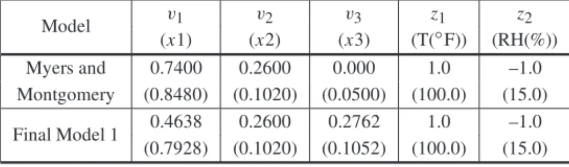
considering the model obtained by Myers & Montgomery (2002) and Final Model 1 obtained in this article. Table 4 presents the optimal values for the components proportions, in L-pseudo components (vi)and in actual values (xi)and the optimal values of the process variables, in coded variables(zi)and in actual values (◦F and RH, respectively).
Table 4– Solution for the maximization problem of example 1.
Model v1 v2 v3 z1 z2
(x1) (x2) (x3) (T(◦F)) (RH(%)) Myers and 0.7400 0.2600 0.000 1.0 –1.0 Montgomery (0.8480) (0.1020) (0.0500) (100.0) (15.0)
Final Model 1 0.4638 0.2600 0.2762 1.0 –1.0 (0.7928) (0.1020) (0.1052) (100.0) (15.0)
Table 5 compares the PRESS, MSE, AI Cc, the response prediction and the variance of a new response for both models. Analyzing the Table 4, we observe that the model obtained in this article presents lower value for PRESS, MSE andAI Cc, emphasizing that was obtained a higher response prediction with a lower variance of a new response.
Table 5– Comparison of two models.
5.1.3 Model Adequacy
The use of studentized residuals to check the normality is recommended by Myers & Mont-gomery (2002). The studentized residuals(ri)are defined as follows:
ri =
ei
ˆ
σ2(1−hii)
(19)
whereei =yi − ˆyi andhii are elements of the hat matrix diagonalsH=W(W′W)−1W′. Figure 1 and 2 present the diagnosis plots used to check the adequacy of the Final Model 1 (a) and the model obtained by Myers & Montgomery (b).
-3 -2 -1 0 1 2 3
-3 -2 -1 0 1 2 3
Studentized Residuals
N
o
rmal P
robabi
lity
(a)
-3 -2 -1 0 1 2 3
-3 -2 -1 0 1 2 3
Studentized Residuals
N
ormal P
robabil
ity
(b)
-3 -2 -1 0 1 2 3
0 10 20 30 40 50 60 70 80 90
Predicted
S
tudent
ized R
e
s
iduals
(a)
-3 -2 -1 0 1 2 3
0 10 20 30 40 50 60 70 80 90
Predicted
S
tudent
ized R
e
s
iduals
(b)
Figure 2– Plot of studentized residualsversusfitted values of Example 1.
In order to check the additivity of the models regarding the linear model, there are the plots of studentized residuals versus fitted values, shown in Figure 2.
The residuals shown in the plot from Figure 2 are randomly distributed around zero. Therefore, the adequacy of Final Model 1 (a) and the model obtained by Myers and Montgomery (b) were checked.
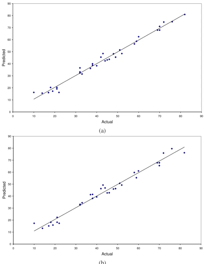
The fitted values shown in the plot from Figure 3 are randomly distributed around actual values. Therefore, the adequacy of Final Model 1 (a) and the model obtained by Myers & Montgomery (b) were checked.
0 10 20 30 40 50 60 70 80 90
0 10 20 30 40 50 60 70 80 90
Actual
P
redict
ed
(a)
0 10 20 30 40 50 60 70 80 90
0 10 20 30 40 50 60 70 80 90
Actual
P
redict
ed
(b)
5.2 Example 2
The problem of Example 2 was presented by Cornell (2000) and Myers & Montgomery (2002). Lauryl sulfate (A), cocamide (B), and lauramide (C) were ingredients in a shampoo whose pro-portionate values were varied in an experiment that was designed to study how shampoo foam height was functionally related to composition. The three ingredients made up 50% of the sham-poo, while the other constituents, which were held fixed in all blends, were water, perfume, and coloring agents.
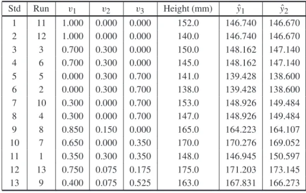
Upper and lower bound constraints were placed on the ingredient or component proportions in the form 0.20≤ A≤0.30, 0.07≤ B ≤0.10, and 0.13≤C ≤0.20, whereA+B+C =0.5. The lower and upper bound constraints, when converted to the mixture components constraints in Eq. (1), are rescaled as 0.40≤ xi ≤ 0.60, 0.14 ≤ x2≤ 0.20, and 0.26 ≤ x3 ≤ 0.40. The experimenter’s objective was to formulate a product with foam height in excess of 170 mm. The authors use L-pseudocomponents and Table 6 presents the experiment.
Table 6– The experiment of Example 2 with L-pseudocomponents for mixture components.
Std Run v1 v2 v3 Height (mm) yˆ1 yˆ2 1 11 1.000 0.000 0.000 152.0 146.740 146.670 2 12 1.000 0.000 0.000 140.0 146.740 146.670 3 3 0.700 0.300 0.000 150.0 148.162 147.140 4 6 0.700 0.300 0.000 145.0 148.162 147.140 5 5 0.000 0.300 0.700 141.0 139.428 138.600 6 2 0.000 0.300 0.700 138.0 139.428 138.600 7 10 0.300 0.000 0.700 153.0 148.926 149.484 8 4 0.300 0.000 0.700 147.0 148.926 149.484 9 8 0.850 0.150 0.000 165.0 164.223 164.107 10 7 0.650 0.000 0.350 170.0 170.276 169.052 11 1 0.350 0.300 0.350 148.0 146.945 150.597 12 13 0.750 0.075 0.175 175.0 171.203 173.145 13 9 0.400 0.075 0.525 163.0 167.831 166.273
The models selected by Cornell (2000) and Myers & Montgomery (2002) both presented PRESS, MSE andAI Cc equal to 657.08, 25.14 and 83.87, respectively, and the model by Cornell (2000) is shown in Eq. (20), while that by Myers & Montgomery (2002) is shown in Eq. (21).
ˆ
y = 94.90+235.05v1+411.42v2−839.41v1v2
−183.21v12−876.64v22+524.99v1v2(v1+v2)
(20)
ˆ
y = 146.74v1+370.32v2+94.90v3+745.43v1v2
+183.21v1v3+876.64v2v3−524.99v1v2v3
(21)
Where
ˆ
y1: Response obtained by Cornell (2000) and Myers & Montgomery (2002) models.
ˆ
5.2.1 Model Selection
All the candidate terms for the ME are the terms in Eq. (3). The model selected according to the
AI Cc criterion was the following:
ˆ
y = 145.89v1+53.69v2+175.89v3+485.98v1v2v3
+353.65v1v2(v1−v2)+190.38v1v3(v1−v3)
(22)
Then, four models are considered non-different. The Model that presents the lowest PRESS (413.22) and MSE (17.09) was selected and named as the Base Model. The Base Model is shown in Eq. (22).
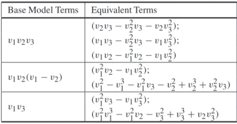
In this step of the methodology we will consider other models using the Base Model. For this, additional terms are generated from the terms of the Base Model. Table 7 presents the equivalent terms to the Base Model terms.
Table 7– Equivalent Terms.
Base Model Terms Equivalent Terms
v1v2v3
(v2v3−v22v3−v2v23);
(v1v3−v22v3−v1v23);
(v1v2−v21v2−v1v22)
v1v2(v1−v2)
(v21v2−v1v22);
(v21−v13−v12v3−v22+v23+v22v3)
v1v3
(v21v3−v1v32);
(v21v31−v21v2−v23+v33+v2v23)
Once all the candidate terms (Base Model terms and Equivalent Terms) for the ME model are known, we may then use the AI Cc criterion again. The model selected is shown in Eq. (23). This model presents PRESS and MSE equal to 348.73 and 16.61, respectively.
ˆ
y = 146.67v1+301.14v2+134.47v3+180.23v21v3−1698.94v23 (23)
We will analyze models considered not different to the model of Eq. (23), as described at the start in Section 5.1.1. The Model that presents the lowest PRESS (348.73) and MSE (16.61) was selected and now, it should be Final Model 2.
Table 8 shows thet-Student test for the Final Model 2.
Table 8– Final Model 2 Test.
Label Estimate Std. Error tvalue p-value v1 146.67 2.61705 56.046 <0.0001 v2 301.14 32.6991 9.209 <0.0001 v3 134.47 4.15726 32.346 <0.0001 v12v3 180.23 30.1357 5.981 0.0003 v32 –1698.94 359.383 –4.727 0.0015
5.2.2 Response Optimization
In the Example 2, a response of exceeding 170 mm is desirable. Several formulations may result in future a response prediction greater than 170 mm. Consequently, a desirable objective is to maximize the expected value for a future response.
The problem may then be formulated as follows:
maxE[ ˆy(w)] =w′βˆ
subject to:
v1+v2+v3=1;
0≤v1≤1;
0≤v2≤0.3;
0≤v3≤0.7.
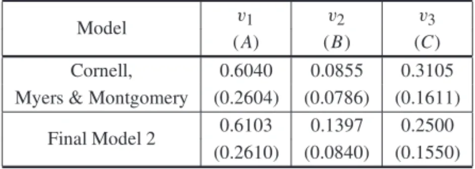
Table 9 presents the optimal values for the components proportions, in L-pseudocomponents
(vi)and in actual values (A, B andC). Table 10 compares the PRESS, MSE, AI Cc, the re-sponse prediction and the variance of a new rere-sponse for three models. Analyzing the Table 9, we observe that the model obtained in this article presents lower value for PRESS, MSE and
AI Cc, emphasizing that was obtained a higher response prediction with a lower variance of a new response.
Table 9– Solution for the maximization problem of Example 2.
Model v1 v2 v3
(A) (B) (C) Cornell, 0.6040 0.0855 0.3105 Myers & Montgomery (0.2604) (0.0786) (0.1611)
Final Model 2 0.6103 0.1397 0.2500 (0.2610) (0.0840) (0.1550)
5.2.3 Model Adequacy
Table 10– Comparison of three models.
Model P R E S S M S E AI Cc var[ ˆy(w)] E[ ˆy(w)] Cornell,
657.08 25.14 83.87 37.7445 174.1457 Myers & Montgomery
Final Model 2 348.73 16.61 56.22 27.8203 177.3530
-3 -2 -1 0 1 2 3
-3 -2 -1 0 1 2 3
Studentized Residuals
N
o
rmal P
robabi
lity
(a)
-3 -2 -1 0 1 2 3
-3 -2 -1 0 1 2 3
Studentized Residuals
N
o
rmal P
robabi
lity
(b)
In the normal probability plot of the studentized residuals shown in Figure 4, we may observe that there isn’t indication that the normality assumption should not be accepted, as there aren’t points way off the alignment.
In order to check the additivity of the model regarding the linear model, there is the plot of studentized residuals versus fitted values, shown in Figure 5.
-3 -2 -1 0 1 2 3
130 135 140 145 150 155 160 165 170 175 180
Predicted
S
tudent
ized R
e
s
iduals
(a)
-3 -2 -1 0 1 2 3
130 135 140 145 150 155 160 165 170 175 180
Predicted
S
tudent
ized R
e
s
iduals
(b)
The residuals shown in the plot from Figure 5 are randomly distributed around zero. Therefore, the adequacy of Final Model 2 (a) and the models obtained by Cornell and, Myers & Montgomery (b) were checked.
The fitted values shown in the plot from Figure 6 are randomly distributed around actual values. Therefore, the adequacy of Final Model 2 (a) and the model obtained by Cornell and, Myers & Montgomery (b) were checked.
130 135 140 145 150 155 160 165 170 175 180
130 135 140 145 150 155 160 165 170 175 180
Actual
P
redict
ed
(a)
130 135 140 145 150 155 160 165 170 175 180
130 135 140 145 150 155 160 165 170 175 180
Actual
P
redict
ed
(b)
Below we present the steps of the methodology proposed in this article:
Step 1: Choose a full model based on Scheff´e’s canonical polynomials for cases of ME, shown in Eq. (3), or choose a full combined model for cases of MPE, shown in Eq. (5), to obtain all the candidate terms.
Step 2: Use the AI Cc criterion and select the model that provides the lowest AI Cc, according to the number of parameters.
Step 3: Calculate the AI Cc differences between the candidate models and the model that
provides the lowestAI Cc and select the non-different models.
Step 4: Analyze the non-different models, and choose the model that provides the lowest MSE and PRESS. This model is now named as the Base Model.
Step 5: Determine all terms that are equivalent to the Base Model terms, and create all the candidate terms.
Step 6: Use the AI Cc criterion again, and select the model that provides the lowest AI Cc according to the number of parameters.
Step 7: Calculate theAI Cc differences between the candidate models and the model that pro-vides the lowestAI Cc and select the non-different models again.
Step 8:Analyze the non-different models, and choose the Final Model that provides the lowest MSE and PRESS.
6 SIMULATION STUDY
A small simulation study is now presented once we know the true model leading to the responses. Considering the experiment of the Table 11 and the true model shown in Eq. (24), we developed a routine in MatlabR to generate the normal responses for this experiment and to select the model
using the proposed methodology.
y=150v1+300v2+150v3+50v1v2−50v1v3+250v12v3−650v22+ε (24)
whereεis the random errors with normal distribution, i.e.ε∼N(0, σ2).
In the simulation study we generated 1,000 experiments with the model shown in Eq. (24), con-sideringσ equal to 0.5 up to 1.5. Using the proposed methodology, the Table 12 shows the identified models with the same terms of the model shown in Eq. (24).
7 CONCLUSIONS
In this article, the statistical techniques necessary for the planning and analysis of mixture experiments with or without process variables were gathered and a methodology for selecting models in MPE and ME was presented with two examples.
Table 11– The experiment of the Simulation Study.
Std v1 v2 v3
1 1.000 0.000 0.000
2 1.000 0.000 0.000
3 0.700 0.300 0.000
4 0.700 0.300 0.000
5 0.000 0.300 0.700
6 0.000 0.300 0.700
7 0.300 0.000 0.700
8 0.300 0.000 0.700
9 0.850 0.150 0.000
10 0.650 0.000 0.350
11 0.350 0.300 0.350
12 0.750 0.075 0.175
13 0.400 0.075 0.525
Table 12–σversusIdentified Models.
σ Identified Models
0.5 1,000
0.6 1,000
0.7 1,000
0.8 1,000
0.9 998
1.0 994
1.1 980
1.2 962
1.3 952
1.4 932
1.5 926
terms of the model may be significant in the presence of some terms and not significant in the presence of other terms. In this context, stepwise forward and backward selection may result in arbitrary selection of variables that belong to the model (Harrell, 2001). An alternative technique was to consider all possible combinations of terms in the full model and the number of parameters and to use selection criteria for models based on Information Theory. From the results obtained in this article, we concluded that the use of the AICc information criterion may result in lower PRESS and MSE.
We may then conclude that the second stage of the methodology provided models that were better than the Base Model and also better than the models obtained previously.
REFERENCES
[1] AKAIKE H. 1973. Information theory and an extension of the maximum likelihood principle, in Mehra RK & Csaki F. (editors),Second International Symposium on Information Theory. Akademiai Kiado, Budapest.
[2] ANDERSON-COOKCM, GOLDFARB HB, BORRORCM, MONTGOMERYDC, CANTER KG & TWISTJN. 2004. Mixture and mixture-process variable experiments for pharmaceutical applications.
Pharmaceutical Statistics,3(4): 247–260.
[3] BORRORCM, MONTGOMERYDC & MYERSRH. 2002. Evaluation of statistical designs for exper-iments involving noise variables.Journal of Quality Technology,34(1): 54–70.
[4] BURNHAMKP & ANDERSONDR. 2002.Model Selection and Multimodel Inference: A Practical Information-Theoretical Approach.Second edition, Springer, New York.
[5] CHUNGPJ, GOLDFARBHB & MONTGOMERYDC. 2007. Optimal Designs for Mixture-Process Experiments with Control and Noise Variables.Journal of Quality Technology,39: 179–190.
[6] CHUNGPJ, GOLDFARBHB, MONTGOMERY DC & BORROR CM. 2009. Optimal Designs for Mixture-Process Experiments Involving Continuous and Categorical Noise Variables.Quality Tech-nology & Quantitative Management,6(4): 451–470.
[7] CORNELL JA. 1995. Fitting models to data from mixture experiments containing other factors.
Journal of Quality Technology,27(1): 13–33.
[8] CORNELLJA. 2000. Fitting a slack-variable model to mixture data: some questions raised.Journal of Quality Technology,32(2): 133–147.
[9] CORNELLJA. 2002.Experiments with Mixtures: Designs, Models and the Analysis of Mixture Data. Third edition, John Wiley and Sons, New York.
[10] CORNELL JA & GORMAN JW. 2003. Two New Mixture Models: Living With Collinearity but Removing its Influence.Journal of Quality Technology,35: 78–88.
[11] DAL BELLO LHA. 2010. Modelagem em Experimentos Mistura-Processo para Otimizac¸˜ao de Processos Industriais. Doctoral Thesis, PUC, Rio de Janeiro.
[12] DALBELLOLHA & VIEIRAAFC. 2011a. Optimization of a product performance using mixture experiments.Journal of Applied Statistics,38(8): 1701–1715.
[13] DALBELLOLHA & VIEIRAAFC. 2011b. Tutorial for mixture-process experiments with an indus-trial application.Pesquisa Operacional,31(3): 1–21.
[14] GOLDFARBHB, BORRORCM & MONTGOMERYDC. 2003. Mixture-Process Variable Experiments with Noise Variables.Journal of Quality Technology,35: 393–405.
[15] GOLDFARB HB, BORROR CM, MONTGOMERY DC & ANDERSON-COOKCM. 2004a. Three-Dimensional Variance Dispersion Graphics for Mixture-Process Experiments.Journal of Quality Technology,36: 109–124.
[17] GOOS P & DONEV AN. 2006. The D-Optimal Design of Blocked Experiments with Mixture Components.Journal of Quality Technology,38: 319–332.
[18] GOOSP & DONEVAN. 2007. Tailor-Made Split-Plot Designs for Mixture and Process Variables.
Journal of Quality Technology,39: 326–339.
[19] HARRELLFE JR. 2001.Regression Modeling Strategies with Applications to Linear Models, Logistic Regression, and Survival Analysis. Springer-Verlag, New York.
[20] HURVICHCM & TSAIC-L 1989. Regression and time series model selection in small samples.
Biometrika,76: 297–307.
[21] KHURI AI. 2005. Slack Variable Models Versus Scheff´es Mixture Models. Journal of Applied Statistics,32: 887–908.
[22] KOWALSKISM, CORNELLJA & VININGGG. 2002. Split-Plot Designs and Estimation Methods for Mixture Experiments with Process Variables.Technometrics,44: 72–79.
[23] MYERSRH & MONTGOMERYDC. 2002.Response Surface Methodology: Process and Product Optimization Using Designed Experiments. Second edition. John Wiley and Sons, New York.
[24] PIEPELGF. 2004. 50 Years of mixture experiment research: 1955–2004, in KHURIAI. (Editor).
Response Surface Methodology and Related Topics. World Scientific Publishing, Singapore, 283– 327.
[25] PIEPELGF. 2007. A Component Slope Linear Model for Mixture Experiments.Quality Technology & Quantitative Management,4(3): 331–343.
[26] PRESCOTTP. 2004. Modeling in Mixture Experiments Including Interactions with Process Variables.
Quality Technology & Quantitative Management,1(1): 87–103.
[27] SAHNINS, PIEPELGF & NÆST. 2009. Product and Process Improvement Using Mixture-Process Variable Methods and Optimization Techniques.Journal of Quality Technology,41(2): 181–197.