Braz. J. Phys. vol.29 número1

Navier-Stokes Equations for Generalized

Thermostatistics

Bruce M. Boghosian

Center for Computational Science, Boston University, 3 Cummington Street, Boston, MA 02215, U.S.A.

Received 07 December, 1998

Tsallis has proposed a generalization of Boltzmann-Gibbs thermostatistics by introducing a family of generalized nonextensive entropy functionals with a single parameter q. These reduce to the extensive Boltzmann-Gibbs form forq= 1, but a remarkable number of statistical and thermody-namic properties have been shown to be q-invariant { that is, valid for anyq. In this paper, we address the question of whether or not the value ofqfor a given viscous, incompressible uid can be ascertained solely by measurement of the uid's hydrodynamic properties. We nd that the hydrodynamic equations expressing conservation of mass and momentum areq-invariant, but the conservation of energy is not. Moreover, we nd that ratios of transport coecients may also be q-dependent. These dependences may therefore be exploited to measureq experimentally.

I Introduction

A. Motivation and Historical Background

The concept of extensivity is introduced early in most textbooks on thermodynamics and statistical physics. The requirement that the entropy be addi-tive establishes the form of the Boltzmann-Gibbs dis-tribution via a straightforward argument. Recently, Tsallis [1] has proposed a generalization of Boltzmann-Gibbs thermostatistics by introducing a family of gen-eralized entropy functionals with a single parameterq.

The proposed generalization is best described by the following two axioms:

Axiom 1

The entropy functional associated with a probability distributionf(

z

)is

S q[

f] k

B q,1

Z

d

z

ff(

z

),[f(

z

)] q

g: (1)

Axiom 2

The experimentally measured value of a phase functiong(

z

)is given by theq-expectation value,

G q[

f] Z

d

z

[f(

z

)] q

g(

z

): (2)

From the rst axiom, we note thatS q[

f] reduces to the

Boltzmann-Gibbs entropy in the limit asq!1,

c S

1[

f] = lim q !1

k B q,1

Z

d

z

ff(

z

),[f(

z

)] q

g=,k B

Z

d

z

f(

z

)lnf(

z

); (3) d

so the generalized thermostatistics includes the usual one as a special case. It diers most notably in the fact that neither the entropy S

q[

f] itself nor the

ob-servablesG q[

f] are extensive thermodynamic variables

when q 6= 1. In spite of this dierence, a

remark-able number of statistical and thermodynamic

prop-erties have been shown to be q-invariant { that is,

valid for any q whatsoever. These include the

name but a few. Other familiar properties, such as the Fluctuation-Dissipation Theorem, are not q-invariant,

but have simple and straightforward generalizations to arbitrary q [4]. The implication is that the

assump-tion of extensivity plays a role analogous to that of the parallel postulate of Euclidean geometry; one can deny it and still get perfectly self-consistent formulations of thermodynamics and statistical physics.

Of course, all this would be but an idle (though undeniably interesting) mathematical exercise unless there were actual physical systems whose thermostatis-tics are best described by the generalized form with

q 6= 1. The exciting realization in recent years is that

there do seem to be some of these. A very abbreviated list of examples is:

Stellar polytropes (e.g., globular clusters) were

long known to possess kinetic equilibria for which there was no corresponding hydrodynamic vari-ational principle until Plastino and Plastino [5] showed that such a variational principle was pos-sible only forq<7=9.

Experimental studies of pure-electron plasmas in

Penning traps have indicated that such plasmas turbulently relax to a radial density prole that does not maximize the Boltzmann-Gibbs entropy. It has recently been shown [6] that the observed proles are consistent with q = 1=2, or perhaps

slightly higher [7].

The ubiquity of Levy ights in physics can be

ex-plained [8, 9, 10] by the fact that they are univer-sal cumulative distributions { in the same sense that the Central Limit Theorem establishes the Gaussian as universal { arising from the general-ized thermostatistics withq>5=3.

Experimental observations of the velocity

distribution of electrons undergoing inverse bremsstrahlung absorption give results consistent withq6= 1 [11].

Two natural questions arise at this point: What characteristics do physical systems with q6= 1 have in

common? Is there a way to predict the value ofq for

a given physical system? Currently, there is more intu-ition about the rst of these questions than the second.

Systems that violate extensivity tend to do so because they have a long-range interaction potential, long-time memory eects, or a fractal space-time structure. The rst of these qualities can make surface eects impor-tant, even in the thermodynamic limit. For example, it is straightforward to show that the total energy of a system of particles inD dimensions with interaction

potential proportional to r

, diverges if

< D [12].

The second quality can invalidate the Markovian as-sumption on which much of our physical intuition is based. The third quality can introduce scaling behav-ior with dimensionality not equal to that of the embed-ding space, and it can invalidate the Ergodic Hypoth-esis which also gures prominently in the justication of the Boltzmann-Gibbs distribution.

B. Planof thisPap er

While it is certainly comforting to nd familiar properties of thermodynamics and statistical mechanics that areq-invariant { because this reinforces our

exist-ing intuition { it is no less important to clearly identify those features that are demonstrably not q-invariant.

To abuse our above analogy with noneuclidean geome-try, these are the phenomena that are the analog of the \triangular excess" of a polygon, or of the curvature tensor. The reason these features are interesting is that they are what allows us to experimentally distinguish systems with dierent values of q. At the level of

ki-netic theory, this is not dicult: The canonical ensem-ble distribution function is q-dependent, so its direct

measurement [11] could provide a way to experimen-tally ascertain q. A more subtle question is whether or

not dierent values ofqcan give rise to dierent

hydro-dynamicbehavior. This is the central question that we address in this paper.

We begin by developing and studying in some de-tail as simple a kinetic theory as we can imagine: We consider an ideal gas for general values ofq. By \ideal"

system, so we are free to mandate thatq6= 1 { at least

as a mathematicalexercise. We may suppose that there is some extenuating circumstance that somehow forces this ideal gas to have q 6= 1. For example, the

parti-cles might well carry a long-term memory of previous collisions, or their geometrical arrangement and/or the shape of their container might conspire to lead to gross violations of the Ergodic Hypothesis. In any case, there is some precedent for using this system to illustrate the application of the generalized thermostatistics: Plas-tino, Plastino and Tsallis [14] considered the partition function and equilibrium properties of this very system, including theq-dependence of its specic heat. In this

paper, we concentrate on the hydrodynamicbehavior of this system.

We next construct a kinetic theory for our general-q

ideal gas. For the sake of simplicity, our kinetic theory is based on the Bhatnager-Gross-Krook (BGK) colli-sion operator, which we generalize to arbitrary q, and

for which we derive a q-invariant H-Theorem. Here it

may be argued that the BGK collision operator is too naive to be used for our purposes, and we ought to have adopted a treatment based on the full Boltzmann equation. In defense of the BGK operator, however, we note that it is well known to produce the correctformof the viscous, compressible Navier-Stokes equations when

q = 1, though the transport coecients are dierent

from those derived by the full Boltzmann treatment. The ratios of the transport coecients, however, are more robust in this regard; for example, both the BGK and Boltzmann treatments for q = 1 yield a ratio of

bulk to shear viscosity of,2=D, even though the

abso-lute values of those viscosities are dierent. For these reasons, we stick to the BGK operator in this paper, focus our attention on robust results such as the form

of the hydrodynamic equations and the ratios of the transport coecients, and leave the more complicated Boltzmann analysis to future studies.

We then derive the viscous, compressible hydrody-namic equations obeyed by the system, using a gener-alization of Chapman and Enskog's asymptotic expan-sion in Knudsen number (the ratio of mean-free path to scale length) [15]. These equations are the general-ization to arbitraryq of the usual Navier-Stokes

equa-tions of hydrodynamics. We nd that the Navier-Stokes equations expressing conservation of mass and

momen-tum areq-invariant, but that for conservation of energy

is not. Moreover, we nd that ratios of transport co-ecients may also beq-dependent. These dependences

may therefore be exploited to measureqby experiments

at the level of hydrodynamics. Finally, in the process of our analysis, we show thatqhas a hard upper bound

of 1 + 2=(D+ 2) for systems of this sort.

II Generalized Hydrodynamic

Equilibria

A. Generalized Thermostatistics

We rst review the construction of the canonical en-semble distribution function using the generalized ther-mostatistics [1]. We maximizeS

q[

f], given by Eq. (1),

subject to the preservation of various linear global func-tionals of f(

z

). By Tsallis' second postulate, Eq. (2),

these are given by

C i q[

f] Z

d

z

[f(

z

)] q

i(

z

)

; (4)

where the indexiranges from 1 to the number of

con-served quantitiesn. We are thus led to the variational

principle,

0 = (

S q[

f], n X i=1

i C

i q[

f] )

; (5)

where the

i's are Lagrange multipliers. It is an

elemen-tary exercise to verify that this yields the equilibrium distribution function

f

(eq )(

z

) = (

q "

1 + (q,1) n X i=1

i k

B

i(

z

) # )

, 1 q ,1

: (6)

The n constants

i are then determined by the n

Eqs. (4) which may be written

C i q=

Z d

z

( q

"

1 + (q,1) n X i=1

i k

B

i(

z

) # )

, q q ,1

i(

z

)

:

(7) In passing, we note that a very recently proposed modication to Tsallis' second axiom [16] would nor-malizetheq-expectation values as follows:

G 0 q[

f] R

d

z

[f(

z

)] q

g(

z

) R

d

z

[f(

z

)] q

This formulation has the virtue of making the q-expectation value of a constant equal to that constant. It has been found by Abe [17] to resolve problems with the niteness of certain physical observables for the general-q ideal gas. It has also been found by Ante-neodo [18] to yield the same dierential equation, albeit with renormalized coecients, for the radial prole of the pure-electron plasma that was found in earlier stud-ies [6, 7]. In this work, however, we shall adhere to the original version of the second axiom. Most of the con-vergence problems encountered in the derivation of the equilibrium properties of the general-q ideal gas [14] do not appear in our derivation of the hydrodynamic properties of that system. So, although the use of nor-malized q-expectation values would be an interesting modication to the current study, we leave it for future

work.

B. Global Hydrodynamic Equilibria

We next consider phase space coordinates

z

= (

x

;

v

), where

x

denotes position and

v

denotes veloc-ity. Because our particles undergo only point collisions, we consider equilibria that conserve mass, momentum and kinetic energy. (We do not have to worry about the potential energy.) That is, we x the q-expectation values of the n = 3 quantities

1(

z

) = m (9)

2(

z

) = m

v

(10)

3(

z

) = mv2=2; (11)

namely

c 0

@

Mq

P

q E

q 1 A

0 @

C1 q

C

2 q

C3 q

1 A

Z

d

z

[f(

z

)]q 0 @

1(

z

)

2(

z

)

3(

z

) 1 A=

Z

d

z

[f(

z

)]q 0 @

m m

v

mv2=2 1

A: (12)

The equilibrium distribution function is then

f(eq )(

z

) =

q

1 + (q,1) m

kB

1+

2

v

+

3

v2

2

,

1 q ,1

: (13)

This may be written in the more concise form

f(eq)(

z

) =

1 + (q,1) m

2kBT

j

v

,

u

j 2

,

1 q ,1

; (14)

where the three quantities

q

1 + (q,1) m

kB

1 ,

2 2

23

, 1 q ,1

(15)

u

,

2

3

(16) and

T

1 3

1 + (q,1) m

kB

1 ,

2 2

23

(17) are determined by the three requirements

0 @

Mq

P

q E

q 1 A= V

q Z

d

v

1 + (q,1) m

2kBT

j

v

,

u

j 2

,

q q ,1

0 @

m m

v

mv2=2 1

A; (18)

and where V R

d

x

is the total spatial volume. The integrals can be done by making the substitution

w

s

m 2kB

q,1

T

(

v

so that 0 @ Mq Pq Eq 1

A= mV q 2kB m T q,1

D= 2 Z dw ,

1 + w2 , q q ,1 0 B B B B @ 1 u+ r 2k B m qT ,1 w u2 2 + r 2k B m qT ,1

uw+k B m qT ,1 w 2 1 C C C C A ; (19)

where we have dened sgn(T=(q,1)) 2 f,1;+1g. The region of integration in w is always spherically

symmetric, so terms with odd integrands vanish, and we may use the D-dimensional spherically symmetric volume element

dw= 2

D=2

,,

D

2 wD

,1dw (20)

on the rest, obtaining

0 @ Mq Pq Eq 1

A = 2mV

q ,, D 2 2kB m T q,1

D= 2 Z

dw wD,1 ,

1 + w2 , q q ,1 0 B @ 1 u u2 2 + kB m qT ,1 w 2 1 C A

= mV _,, q

D 2 2kB m T q,1

D= 2 Z

dx xD=2,1

(1 + x), q q ,1 0 B @ 1 u u2 2 + kB m qT ,1 x 1 C

A; (21)

where xw 2.

At this point, we need to specify the limits of integration. If = +1, the integrand is dened for 0x <1. If

=,1, then the integrand is dened only for 0x1. In the latter case, states with x > 1 or

jv,uj> s 2kB m T q,1

(22)

arethermally forbidden. Thus, we have

0 @ Mq Pq Eq 1

A= mV

q

,,D 2 2kB m T q,1

D= 2 8 > > > > > > > > < > > > > > > > > : R 1 0 dx x

D=2,1(1 + x) , q q ,1 0 B @ 1 u u2 2 + kB m qT ,1 x 1 C

A for = +1 R

1 0 dx x

D=2,1(1 ,x) , q q ,1 0 B @ 1 u u2 2 + kB m qT ,1 x 1 C

A for = ,1

(23) In both cases, the integration results in a beta function, and this can be expressed in terms of gamma functions [13]. The results are

0 @ Mq Pq Eq 1

A= mV q

2kBT

m D=2 8 > > > > > > > > < > > > > > > > > : ,( q q ,1 , D 2) jq,1j

D =2 ,(

q q ,1)

0 B @ 1 u u2 2 +

DkBT= (2m)

q,(q,1)( D

2 +1)

1 C

A for = +1 ,(

1 1,q) j1,qj

D =2 ,( 1 1,q + D 2) 0 B @ 1 u u2 2 +

DkBT= (2m) 1+(1,q)

D 2

1 C

A for = ,1

(24)

In either case, we see that the momentum per unit mass, or hydrodynamic velocity, is given by

u q

P

q

Mq

=u: (25)

The energy per unit mass is then "q

E

q

Mq

= u2 q

2 + q; (26)

where we have dened the thermal or internal energy per unit mass,

q

DkBT

2m

1 + (1,q) D2

,1

(27) which, remarkably, is independent of .

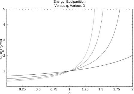
At this point, we arrive at an interesting ambigu-ity. We are tempted to interpret the variable that has been suggestively called T as the temperature of our physical system. Certainly, it reduces to the usual tem-perature for q = 1. If we make this interpretation, we might conclude that the familiar energy equipartition theorem is invalid for q6= 1. That is, for general q the

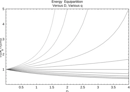
thermal energy per unit mass is apparently no longer directly proportional to the dimension D. Figs. (1,2) plot the ratio q=(DkBT=(2m)) versus (q;D) for

vari-ous values of (D;q), respectively. This ratio is equal to

unity when equipartition holds. We see that it is less than unity for q < 1, and greater than unity for q > 1. We may even be tempted to attach physical signicance to this result by noting that the equipartition theorem presumes ergodicity, and systems with q 6= 1 are

gen-erally not ergodic. This reasoning is faulty, however, because it depends upon our rather arbitrary denition of the temperature in terms of the Lagrange multipliers in Eq. (17). If we had instead dened the temperature as

T0

T 1 + (1,q)

D 2

; (28)

which also reduces to the usual denition as q ! 1,

we would have found that q = DkBT

0=(2m) and

con-cluded that equipartition is valid for all q. The lesson here is that the denition of the temperature is rather arbitrary in thermodynamics, and we should not sup-pose that we can measure its absolute value in an ex-periment. So, even though we have theoretical reason to believe that q(T) is q-dependent, we can not exploit

this dependence to measure q experimentally. To do that, it will be necessary to nd two physical observ-ables whose relationship to each otheris q-dependent. We shall return to this point numerous times below.

0.25 0.5 0.75 1 1.25 1.5 1.75 2

q 1

2 3 4 5

ι/

(Dk T/(2m))

B

Energy Equipartition Versus q, Various D

0.5 1 1.5 2 2.5 3 3.5 4 D

1 2 3 4 5

ι/

(Dk T/(2m))

B

Energy Equipartition Versus D, Various q

Figure 2. A plot of the ratio q=(kBT=(2m)) versusDforq ranging from 0:2 to 2:0 in increments of 0:2. The plot color becomes lighter asqincreases.

We also note from Eq. (27) that there is a hard up-per bound on q for this type of system. In order for the proportionality constant between q and T not to

become negative, it must be that 1 + (1,q)D=2 > 0,

or

q < 1 + 2D: (29) This conclusion is independent of dieomorphic

trans-formations in our denition of T and therefore may be expected to have some general validity 1. A similar

inequality was derived in [14]. We shall show below that hydrodynamic considerations { in particular, the positivity and niteness of the thermal conductivity { impose an even more stringent upper bound on q.

Finally, the normalization constant can be ex-pressed in terms of the mass density q

M

q

V as follows

q = q

m

m 2kBT

D =2 8 > > > < > > > :

jq ,1j D =2

,( q q ,1) ,(

q q ,1

, D 2)

for = +1

j1,q j D =2

,( 1 1,q

+ D

2) ,(

1 1,q)

for =,1

(30)

It follows that the global hydrodynamic equilibrium (GHE) distribution function can be written in the form

f(eq )( z) =

"

cq ;Dq

m

m 2kBT

D =2 #1

q

1 +

q,1

kBT

m 2 jv,u

q j

2

, 1 q ,1

; (31)

where we have dened

d

1Of course, it could well be that we want to generalize our notion of temperature to include negative values, in which case this upper

c q ;D

8 > > > < > > > :

jq ,1j D =2

,( q q ,1) ,(

q q ,1

, D

2)

for= +1 j1,q j

D =2 ,(

1 1,q

+ D

2) ,(

1 1,q)

for=,1,

(32)

and with the proviso thatf (eq )(

z) = 0 if the argument

raised to the,1=(q,1) power in Eq. (31) is negative.

This is the generalization of the Maxwell-Boltzmann distribution function for the Generalized

Thermostatis-tics. The coecients c

q ;D have a particularly simple

form for even dimensionD,

c q ;D =

D =2 Y `=1

[`,(`,1)q]; (33)

in particular, we note that c

q ;2 = 1 and c

q ;4 = 2 ,q.

More generally, these coecients are plotted againstq

for various values ofD in Fig. 3. Various distributions

forD= 1 are illustrated in Figs. 4 and 5.

0.5 1 1.5 2 2.5 3

q 0.25

0.5 0.75 1 1.25 1.5 1.75 2

c

q,D

Coefficient c Versus q, Various D q,D

Figure 3. A plot of the coecients c

q ;Dversus

qforDranging from 1 to 4. The plot color becomes lighter asDincreases.

-4 -2 0 2 4

v 0

0.1 0.2 0.3 0.4

[f(v)]

q

Generalized Distribution Function Fixed u and T, Varying q

Figure 4. A plot of [f (eq)(

z)] q versus

-4 -2 0 2 4 v

0 0.1 0.2 0.3 0.4 0.5 0.6 0.7

[f(v)]

q

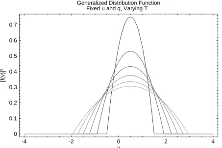
Generalized Distribution Function Fixed u and q, Varying T

Figure 5. A plot of the equilibrium distribution function versusvforD= 1,q= 1,uq = 1=2,q= 1=2 andT ranging from 0:25 to 1:5 in increments of 0:25. The plot color becomes lighter asT increases.

III Generalized Kinetics

A. Local Hydrodynamic Equilibria

Before introducing our generalization of the BGK collision operator, we rst introduce the concept of lo-cal hydrodynamic equilibrium (LHE). The GHE distri-bution function derived in the preceeding section is a function of velocity

v

alone, and independent of posi-tion

x

. This is a direct consequence of the fact that the only conserved quantities present { mass, momentum and kinetic energy { are functions of

v

and not of

x

. The GHE distribution does depend parametrically on q,

u

q and "q, so we may write it in the more precise

for-mat f(eq )(

v

;

q;

u

q;"q). The LHE distribution function

f(0)(

z

) is then dened as having the same functional

form as the GHE, but with parameters q,

u

q and "q

weakly dependent on spatial position

x

. That is, f(0)(

z

) = f(eq )(

v

;

q(

x

);

u

q(

x

);"q(

x

)): (34)

It should be noted that the LHE, unlike the GHE, is

notexpected to be a stationary state of the system. If the system is initialized in a LHE distribution, its time evolution will generally take it away from this simple functional form. That is, the full solution to the sys-tem's kinetic equation should be expected to be the LHE plus a correction. To the extent that the spatial gradients are weak, this correction will be small and can be treated perturbatively. This is the basis of the Chapman-Enskog expansion.

B. The Generalized BGK Equation and

H

-Theorem

Armed with the concept of LHE, we propose the fol-lowing generalization of the Boltzmann equation with the BGK collision operator:

c

@

@t +

v

r

[f(

z

)]q

=,

1

n

[f(

z

)]q ,

h

f(0)(

z

) i

q o

; (35)

where f(0)(

z

) is the LHE distribution function that is dened as having the same moments as the exact distribution

function f(

z

), 0 @

q

q

u

q

q"q 1 A=

Z

d

v

[f(

z

)]q 0 @

m m

v

mv2=2 1 A=

Z

d

v

h

f(0)(

z

) i

q 0 @

m m

v

mv2=2 1

A; (36)

determine the parameters that appear nonlinearly in its functional form, are themselves functionals of f(z). To

see this more clearly, note that Eqs. (34) and (36) can be used to rewrite Eq. (35) in the explicitly nonlinear but woefully cumbersome form

@

@t +vr

[f(z)] q

=,

1

[f(z)] q

,

f(eq )

v; Z

dv[f(z)] qm;

Z

dv[f(z)] qm

v; Z

dv[f(z)] qm

2 v2

q

: (37) Hence, when q6= 1, this departs from the usual BGK equation in two important respects: First, and most obviously,

it is constructed so that it relaxes to the explicitly q-dependent LHE f(0)(

z), given by Eqs. (34) and (31), rather than

to the usual Maxwell-Boltzmann LHE. Second, the nonlinearity in the collision operator arises via the functional form of [f(0)]q which also explicitly depends on q. It is important to keep these two mechanisms clearly in mind

because a supercial glance at Eq. (35) might suggest that the substitution F(z)[f(z)]

q will render its dynamics

identical to those of the usual BGK equation, and this is not so.

Eq. (35) is a sensible generalization of the BGK equation for three reasons. First, it obviously reduces to the usual BGK equation when q = 1. Second, if we multiply it by the i(

z) and integrate overv, we nd local

conservation equations

0 = @@t

0 @ q( x) p q( x)

"q( x)

1 A+

r Z

dv [f(z)] q

0 @

mv

mvv

mvv 2=2

1

A (38)

for each of the conserved quantities. Third, we can show that Eq. (35) obeys an H-theorem { at least for q > 0 { as follows:

d

dtSq[f] = Z

dz

Sq[f]

f(z)

@f(z)

@t = kB

q,1 Z

dz

1,q[f(z)]

q ,1 @f( z)

@t = kB

q,1 Z

dz

1 q[f(z)]

q ,1 ,1

@ @t[f(z)]

q

= kB

q,1 Z

dz

1 q[f(z)]

q ,1 ,1

@

@t +vr

[f(z)] q

= ,

kB

(q,1) Z

dz

1 q[f(z)]

q ,1 ,1

n

[f(z)] q ,[f (0)( z)] q o

= Sq

f(0)

,S q[f]

+ kB

(q,1) Z

dz

h

f(z),f (0)(

z) i

,

[f(z)] q

,[f (0)(

z)] q

q[f(z)] q ,1

= Sq

f(0)

,S q[f]

+ kB

(q,1) Z

dzf (0)(

z)

[g(z),1],

[g(z)] q

,1

q[g(z)] q ,1

= Sq

f(0)

,S q[f]

+ kB

Z

dzf (0)(

z) q(g(

z)) ; (39)

d

where g(z) f(z)=f (0)(

z) > 0, the domain has been

assumed to be without boundary, and where we have dened the function

q(x)

1 q,1

(x,1),

xq ,1

qxq ,1

: (40) The rst term of Eq. (39) is nonnegative since the en-tropy is a maximumfor the distribution function f(0)(

z)

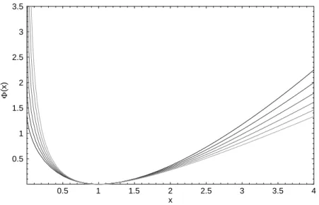
and q > 0 by construction. It is not dicult to show that the function q is nonnegative for positive

argu-ment (see Fig. 6), so the second term is also

nonneg-ative. It follows that dSq[f]=dt

0 for q > 0, with

equality holding only at equilibrium.

For q < 0, the generalized entropy Sq[f] is

mini-mizedat its extremum, rather than maximized, as can be seen from examination of its second variation. In this situation, the rst term on the right-hand side of Eq. (39) is negative, but the second term is still posi-tive because q(x)

0 still holds for q0. Hence the

0.5 1 1.5 2 2.5 3 3.5 4 x

0.5 1 1.5 2 2.5 3 3.5

Φ

(x)

Figure 6. A plot of the function q(

x) versusxforq2f0:25;0:50;0:75;1:00;1:25;1:50g. The plot color becomes lighter asq increases.

IV The Chapman-Enskog

Anal-ysis

A. The Asymptotic Expansion

We now develop the distribution function in a per-turbation series where the zero-order approximation is the LHE, following the program described in Subsec-tion III. We rewrite our generalized BGK equaSubsec-tion, Eq. (35), in the form

1 +D^

F(

z

) =F (0)(

z

)

; (41)

where we have dened

F(

z

) [f(

z

)] q

(42) and

(43)

F (0)

(

z

) h

f (0)

(

z

)i q

; (44)

and the operator ^

D

@ @t

+

v

r: (45)

The formal solution to the above equation is

F(

z

) =

1 +D^

,1 F

(0)(

z

)

: (46)

Following the standard Chapman-Enskog proce-dure [15], we expand the derivative in a series of suc-cessively more slowly varying time scales,

^

D= 1 X j=1

j^ D j

; (47)

where

^

D j

@ @t j

+

v

r; (48)

whereis a formal expansion parameter, andt j is the jth time scale. To second order in, we nd

F(

z

) = h

1,D^ 1

, 2

^

D 2

,D^ 2 1

+ i

F (0)(

z

)

:

(49) Thus we have

F(

z

) = 1 X n=0

n F

(n)(

z

)

; (50)

where

F

(1)(

z

) = ,D^

1 F

(0)(

z

) (51)

F

(2)(

z

) = ,

^

D 2

,D^ 2 1

F (0)(

z

)

: (52)

... The higher order termsF

(1)and F

(2)must not change

0 =Z

dv h

F(z),F (0)(

z) i

0 @

mv

mvv

mvv 2=2

1 A=

1 X n=1

n Z

dvF (n)(

z) 0 @

mv

mvv

mvv 2=2

1

A: (53)

To fully specify the determination of the F(n), we further require that they satisfy Eq. (53) order by order; that is,

0 =Z

dvF (n)(

z) 0 @

mv

mvv

mvv 2=2

1

A (54)

for n1.

B. TheFirst-OrderSolution

At rst order, Eq. (51) can be written F(1)(

z) =,

@ @t1

+vr

F(0)(

z): (55)

We take the hydrodynamic moments of both sides, noting that the left-hand side will vanish thanks to Eq. (54). We get

0 = @@t1 0 @

q

q u

q

q"q 1 A+

r Z

dvF (0)(

z) 0 @

mv

mvv

mvv 2=2

1

A: (56)

The rst of these is immediately seen to be the usual equation expressing conservation of mass 0 = @q

@t1

+r( q

u

q); (57)

which is thus seen to be q-invariant at rst order.

To evaluate the momentum equation at rst order, we must integrate the dyad mvvtimes F

(0). We have Z

dvF (0)(

z)mvv = Z

dvF (0)(

z)m[(v,u q) +

u q][(

v,u q) +

u

q] (58)

= q u

q u

q+

2kB

m

T q,1

D 2

+1 Z

dwF (0)(

z)mww; (59)

since the odd cross terms integrate to zero. Turning our attention to the last integral overw, it is clear from parity

that only the diagonal elements of this dyad will have nonvanishing integral, and from isotropy that they will all give the same result. Thus, we have

Z

dvF (0)

(z)mvv= q

u q

u q+

1

2kB

m

T q,1

D 2

+1 Z

dwF (0)

(z)mw 2

x: (60)

d

To perform this last integral, the spherically sym-metric volume element of Eq. (20) is inadequate. Rather, we write wx = w cos, where 0

is

a polar angle, and we adopt the cylindrically symmet-ric volume element

dw= 2 D ,1

2

,, D ,1

2 w

D ,1dw d: (61)

Now both the w and integrals yield beta-functions

which must be considered for both cases =1. The

result, which does not depend on , is then

Z

dvF (0)(

z)mvv= q

u q

u q+ Pq

1 (62)

where we have dened the pressure

Pq

qkBT

m

1 + (1,q) D

2

The momentum equation at rst order is thus 0 = @@t1

(q u

q) + r(

q u

q u

q+ Pq

1): (64)

Eq. (63) appears to be a nonideal equation of state for the pressure but, as noted at the end of the previ-ous subsection, we must avoid attaching physical signif-icance to the temperature T. Rather, we should take care to relate observable quantities { in this case, the pressure Pq and the internal energy q. From Eqs. (63)

and (27), we have

Pq = 2Dqq; (65)

and this is the usual ideal gas equation of state with no correction, which we see is q-invariant after all.

Finally, we consider the energy equation at rst or-der. We must integrate the vector mvv

2=2 times F(0).

We have

c Z

dvF (0)( z)m vv 2 2 = Z

dvF (0)(

z)m2 [(v,u q) +

u q]

j(v,u q) +

u q

j 2

(66)

= q"q u q+ u q " 2kB m T q,1

D 2 +1 Z

dwF (0)(

z)mww #

(67)

since the odd cross terms integrate to zero. The quan-tity in square brackets in the second term is the same one we encountered in the denition of the pressure and is equal to Pq

1. The energy equation at rst order is

thus

0 = @_@t

1

(q"q) + r[(

q"q+ Pq) u

q]: (68)

Eqs. (57), (64) and (68) give us the rate of change of the hydrodynamic variables on time scale t1. They

and the equation of state, Eq. (65), are all seen to be

q-invariant. Thus, at rst order, there is no experiment that we could perform that would distinguish a system with q6= 1 from the more orthodox q = 1 case. To make

this distinction, we must examine the dissipative terms that appear at second order in the Chapman-Enskog analysis, and we turn our attention to those now.

C.The Second-OrderSolution

At second order, Eq. (52) can be written

c

F(2)(

z) =, "

@ @t2

+vr

F(0)( z),

@ @t1

+vr

2

F(0)( z)

#

: (69)

Again, we take the hydrodynamic moments of both sides, noting that the left-hand side will vanish thanks to Eq. (54). Drawing on our experience from the rst-order calculation, we see that we get

@ @t2 0 @ q q u q

q"q 1 A+ r 0 @ q u q q u q u

q+ Pq 1

(q"q+ Pq) u q 1 A = 2 4@ 2 @t2 1 0 @ q q u q

q"q 1 A+ 2 @

@t1 r 0 @ q u q q u q u

q+ Pq 1

(q"q+ Pq) u q 1 A+ rr: Z

dvvvF (0)( z) 0 @ m mv

mv2=2 1 A 3 5

= r 2 4 @ @t1 0 @ q u q q u q u

q+ Pq 1

(q"q+ Pq) u q 1 A+ r Z

dvvvF (0)( z) 0 @ m mv

mv2=2 1 A 3

5; (70)

where we used the rst order results in the second step. Note that the right-hand side is now manifestly a divergence. The quantity inside this divergence is the negative of a diusive ux. The derivatives with respect to t1 can be

The right-hand side of the second-order mass conservation equation is seen to vanish due to the rst-order momentum conservation equation. Thus, we nd that the form of the mass conservation equation

0 = @q

@t2

+r( q

u

q) (71)

is q-invariant to second order.

To evaluate the right-hand side of the momentum equation at second order, we must integrate the triad mvvv

times F(0). The procedure is the same as that at rst order, and no new moments need to be dened. The result

in index notation is

Z

dvF (0)(

z)mv

ivjvk = quq iu

q ju

q k+ P

q

ijuq k+

ikuq j+

jkuq i

: (72)

Inserting this into the second-order momentum equation, carrying out the derivatives with respect to t1 using the

rst-order equations, and simplifying, we get @

@t2

(q u

q) + r(

q u

q u

q+ Pq

1) =r n

q h

ru q+ (

ru q)

T i

+ q( ru

q) 1

o

; (73)

where the superscript T denotes \transpose," and where we have dened theshear viscosity

q

2

D qq; (74)

and thebulk viscosity

q

,

4 D2

qq: (75)

Here we have used the equation of state, Eq. (65), to express the viscosities in terms of the internal energy. Note that Eqs. (74) and (75) are q-invariant, as is the ratio

q

q

=,

2

D (76)

which is known to be approximately true for a variety of real gases [19]. Thus, measurement of the ratio of the viscosities is still insucient to determine q experimentally.

Finally, we turn our attention to the energy equation at second order. For this we must integrate the dyad mvvv

2=2 times F(0). The by now familiar procedure again yields beta-function integrals which must be considered

for both cases =1. The result, which does not depend on , is then Z

dvF (0)(

z)mvv

v2

2 = (q"q+ 2Pq) u

q u

q+ (

Pq

u2 q

2 +D42

D 2 + 1

"

1 + (1,q) D

2

1 + (1,q) ,

D 2 + 1

#

q 2 q

)

1: (77)

Inserting this into the second-order energy equation, carrying out the derivatives with respect to t1 using the

rst-order equations, and simplifying, we get @

@t2

(q"q) + r[(

q"q+ Pq) u

q]

= r

u q

h

q

ru q+ (

ru q)

T

+ q( ru

q) 1

i

+ kq r

q

,(1,q)a q

q r(

qq)

(78)

d

where we have dened thethermal conductivity

kq

4 D2

1 + D2 "

1 + (1,q) D

2

1 + (1,q) ,

D 2 + 1

#

qq; (79)

and the anomalous transport coecient

aq

4 D2

"

D 2 + 1

1 + (1,q) ,

D 2 + 1

#

We note that positivity and niteness of the thermal conductivity sets an even more stringent upper bound onq than Eq. (29), namely

q<1 + 2 D+ 2

: (81)

We emphasize that this inequality is not expected to hold for general systems; its derivation was specic to our assumption of an ideal gas.

The most striking feature of the second-order en-ergy conservation equation, Eq. (78), is that it is not q-invariant. Its diusive ux contains a term

propor-tional to (1,q)r( q

q)

=

q with a new transport

co-ecient a

q. The presence of this term can be detected

by purely hydrodynamic experiments and this may be used to test whether or notq is equal to unity.

More-over, we see that the ratio

a q k

q

=

1 + (1,q) D

2

,1

(82) gives us another means of determining q, as does the

ratio

k q

q

= 2

D

D

2 + 1

"

1 + (1,q) D

2

1 + (1,q) ,

D 2 + 1

#

: (83)

These ratios are plotted in Figs. 7 and 8.

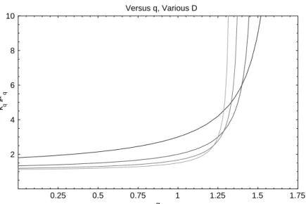
0.5 1 1.5 2 2.5 3

q 2

4 6 8 10

a /k q q

Ratio a /k q q

Versus q, Various D

Figure 7. A plot of the ratio of the anomalous transport coecienta

q to the thermal conductivity k

q for

Dranging from 1 to 4. The plot color becomes lighter asDincreases.

0.25 0.5 0.75 1 1.25 1.5 1.75

q 2

4 6 8 10

k /

µ q q

Ratio k / µ

q q

Versus q, Various D

V Discussion

Eqs. (71), (73) and (78) constitute the compressible Navier-Stokes equations for the generalized thermo-statistics. We see that the mass and momentum con-servation equations are completelyq-invariant, but the

energy conservation equation is not. It contains a term that is proportional to (1,q)r(

q

q) =

q which

van-ishes for Boltzmann-Gibbs statistics. It is a term not normally included in presentations of the Navier-Stokes equations.

In addition, we have shown that certain ratios of the transport coecients may be q dependent. While the

famous result q

= q =

,2=Dappears to beq-invariant,

the ratiosk q

= qand

a q

=k

q are decidedly less robust and

may be used to infer a value of q. At this point, the

reader may be tempted to pick up a handbook of ma-terial properties, search for mama-terials with anomalous ratios of thermal conductivity to shear viscosity, and at-tribute those anomalies to a breakdown in Boltzmann-Gibbs statistics for those materials. The reader is implored to resist this temptation. There are very many potential pitfalls in the Boltzmann/Chapman-Enskog analysis that are far more likely to generate such anomalies than a breakdown in the foundations of ther-mostatistics. The presence of rotational and/or internal molecular degrees of freedom, high densities leading to three-body collisions, and violations of the Boltzmann molecular chaos assumption are but three examples of phenomena that might also cause such anomalies. If, however, one has other reasons to believe that a particu-lar system violates Boltzmann-Gibbs thermostatistics, then examination of the ratios of the transport coef-cients may provide further corroboration. One does have such reason to believe this for the stellar polytrope and pure-electron plasma examples mentioned earlier; unfortunately, those systems of particles are not ideal gases in any reasonable sense of the term so, even if one could measure the transport coecients of such things, the quantitative results derived above should not be expected to apply.

In summary, the presence of the anomalous term in the energy equation of a dilute gas would seem to be the easiest way to search for deviations ofqfrom unity.

I am currently unaware of any experimental work that would clearly establish either the presence or absence of this term. I leave it to my colleagues who have more familiarity with the experimental hydrodynamic litera-ture to sort out this matter.

VI Conclusions

We have shown that the Navier-Stokes equations for mass and momentum conservation are q-invariant to

second order in the Chapman-Enskog expansion, but that the equation for energy conservation is not. We have derived the form of this anomalous term, using a generalized Chapman-Enskog analysis on a generalized BGK kinetic equation. In addition, we have found q

-dependent anomalies in ratios of certain transport co-ecients { in particular, in the ratio of the thermal conductivity to the shear viscosity. Finally, we have found that hydrodynamics gives rise to the upper bound

q <1 + 2=(D+ 2) which is more stringent than that

imposed by equilibrium considerations.

This work could be substantially improved by using a more realistic kinetic equation, but we have argued that the principal results { the form of the hydrody-namic equations, and theratiosof the transport coe-cients { ought to be robust in this regard. It is hoped that some of the insights obtained in this analysis will eventually be useful in constructing simple experimen-tal tests for the presence of breakdowns in Boltzmann-Gibbs statistics.

VII Acknowledgements

The author would like to thank Constantino Tsallis and Lisa Borland for their careful reading of the original draft of this paper, and for their helpful suggestions. The author would also like to thank Celia Anteneodo for sharing the results of her recent recalculation of the radial prole of the pure-electron plasma using normal-izedq-expectation values [18].

References

[1] C. Tsallis,J.Stat.Phys.52(1988) 479;PhysicaA221 (1995) 277.

[2] E.M.F. Curado, C. Tsallis,J.Phys.A:Math.Gen.24 L69.

[3] A. Chame, E.V.L. de Mello,Phys. Lett.A228(1997) 159.

[4] A. Chame, E.V.L. de Mello,J.Phys.A27(1994) 3663. [5] A.R. Plastino, A. Plastino, Phys. Lett. A174 (1993)

384-386.

[6] B.M. Boghosian, Phys.Rev.E53(1996) 4754-4763. [7] C. Anteneodo, C. Tsallis, J.Mol. Liq.71(1997)

[8] P.A. Alemany, D.H. Zanette, (1994) R956.

[9] C. Tsallis, S.V.F. Levy, A.M.C. de Souza, R. Maynard, Phys.Rev.Lett.75(1995) 3589; Erratum: Phys.Rev. Lett.77(1996) 5442.

[10] C. Tsallis,PhysicsWorld(July, 1997) 42.

[11] C. Tsallis, A.M.C. de Souza,Phys.Lett.A235(1997) 444-446.

[12] N. Goldenfeld, \Lectures on Phase Transitions and the Renormalization Group," Addison-Wesley (1992) 27-28.

[13] M. Abramowitz and I.A. Stegun, \Handbook of Math-ematical Functions," National Bureau of Standards (ninth printing, 1970) p. 258.

[14] A.R. Plastino, A. Plastino, C. Tsallis, Math.Gen.27(1994) 5707-5714.

[15] K. Huang, \Statistical Physics," John Wiley and Sons (third printing, 1966).

[16] C. Tsallis, R.S. Mendes, A.R. Plastino,PhysicaA261 (1998) 534.

[17] S. Abe, \Thermodynamic Limit and Classical Ideal Gas in Nonextensive Statistical Mechanics with Nor-malisedq-Expectation Values," preprint (1998). [18] C. Anteneodo, private communication (1998).