Adv. Radio Sci., 5, 127–133, 2007 www.adv-radio-sci.net/5/127/2007/ © Author(s) 2007. This work is licensed under a Creative Commons License.
Advances in
Radio Science
Extended post processing for simulation results of FEM synthesized
UHF-RFID transponder antennas
R. Herschmann1,2, M. Camp1,2, and H. Eul1
1Leibniz Universit¨at Hannover, Institute of Radiofrequency and Microwave Engineering, Appelstraße 9a, 30167 Hannover, Germany
2Smart Devices GmbH & Co. KG, Sch¨onebecker Allee 2, 30823 Garbsen, Germany
Abstract. The computer aided design process of sophisti-cated UHF-RFID transponder antennas requires the applica-tion of reliable simulaapplica-tion software. This paper describes a Matlab implemented extension of the post processor capa-bilities of the commercially available three dimensional field simulation programme Ansoft HFSS to compute an accurate solution of the antenna’s surface current distribution. The accuracy of the simulated surface currents, which are phys-ically related to the impedance at the feeding point of the antenna, depends on the convergence of the electromagnetic fields inside the simulation volume. The introduced method estimates the overall quality of the simulation results by com-bining the surface currents with the electromagnetic fields extracted from the field solution of Ansoft HFSS.
1 Introduction
The development and optimization of passive transponders for application in UHF-RFID systems with wide read range is directly correlated to the supply of appropriate antenna de-signs. On the one hand these antennas must be frequency selective in order to suppress interferences of radio systems in adjacent wave bands. Otherwise the antennas should ex-hibit enough bandwidth to compensate for tolerances of chip impedance and to account for the influence on impedance from the adjacencies of the antenna. A largely stable use of a passive transponder makes sense in a moderately variable environment only in such a way. The dependence between geometry and impedance qualities of the antenna makes the synthesis of suitable antenna structures possible for the ful-filment of the qualification profile under consideration of the at most permitted geometric measurements.
Correspondence to:R. Herschmann ([email protected])
The design process of a transponder antenna for the ap-plication in an UHF-RFID system using the Finite Element Method (FEM) allows for the consideration of extended, ge-ometrical complex objects with arbitrary material character-istics in the near field region. The material specific quali-ties of these objects generally lead to an impact on the an-tenna impedance associated with changes of the resonant frequency, bandwidth and matching between antenna and transponder chip. Recent simulation programmes allow for an optimization of the antenna design by the variation of de-fined geometry parameters of simulation models parameter-ized correspondingly under consideration of predefined en-vironmental conditions.
128 R. Herschmann et al.: Extended post processing of FEM based simulation results
λ
Fig. 1.Convergence of the electromagnetic field at defined observation points versus the number of adaptive passes; while the electric field shows well convergence properties in(a), the magnetic field shows substantial changes in(b).
λ
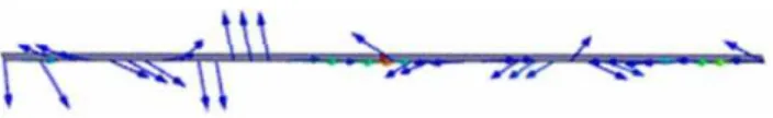
Fig. 2.Surface current distribution of aλ/2-dipole at resonant fre-quency extracted from Ansoft HFSS.
2 HFSS simulation results: convergence of electromag-netic fields and impedance
It is appropriate to clarify the necessity for dealing with the subject of field and impedance convergence by observing the simulation results for a simple resonant dipole antenna using HFSS. The surface current distribution of that antenna is well known to be sinusoidal along the dipole’s centre line (see Stutzman and Thiele, 1998). In Fig. 1 the Cartesian compo-nents of the electromagnetic fields are represented. While the observation points of the electric field are distributed inside the simulation volume, the magnetic fields are com-puted along the antenna surface. The electromagnetic fields are plotted against the number of adaptive passes. In con-trast to the electric fields the magnetic fields show substantial changes in field magnitudes even at a high number of adap-tive passes. HFSS computes the surface current distribution by processing the magnetic fields on the antenna structure. But the results for two dimensional antennas with neglected
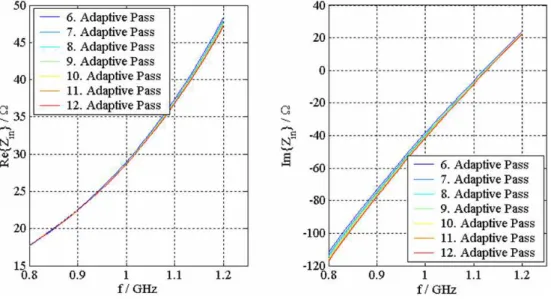
metal thickness are not correct as depicted in Fig. 2. On the other hand convergence of the impedance at the antenna’s feeding point shown in Fig. 3 is already reached within a few adaptive passes. Due to the physical relation between an-tenna impedance and anan-tenna surface current distribution it is appropriate to check the field solution.
3 HFSS eXtension Module: a Matlab implemented pro-cedure for post processing FEM based simulation re-sults
R. Herschmann et al.: Extended post processing of FEM based simulation results 129
Fig. 3.Impedance convergence at the antenna’s feeding point versus the number of adaptive passes.
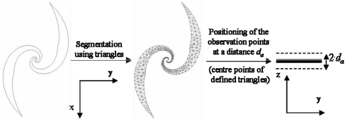
Fig. 4. Ansoft HFSS simulation model of the spiral antenna and distribution of the observation points inside the simulation volume (blue markers represent observation points for the electric field, red markers are used for the magnetic field).
3.1 The principle of the calculation method
The Matlab procedure performs a comparison between the electric fields taken directly from the solution of the finite el-ement method implel-emented in HFSS and the electric fields which are derived from the distribution of the antenna’s sur-face currents. To this end a suitable observation point area has to be defined within the boundaries which are provided by the used simulation model. It is possible to use different geometries for this observation point area, e.g. lines, planes or cuboids. The higher the dimension of this geometrical structure chosen as the observation point area the better the results regarding the corrected surface current distribution. The electric fields are used for comparison because HFSS de-termines the magnetic fields by a numeric calculation based on the solution of the electric fields. The electric fields are
therefore computed with a higher precision. Aim of the pro-cedure is the optimization of a scaling factor applied to cal-culated initial surface current distribution in order to min-imize the difference between the compared electric fields. This initial current distribution of the antenna is calculated from the magnetic fields in close proximity to the antenna surface. As a working example the method is applied to the analysis of the field convergence of a two arm spiral an-tenna. The equally spaced observation points of the elec-tric fieldsE=h (f,ra2)are positioned between an inner and outer cuboid. The observation points of the magnetic fields
130 R. Herschmann et al.: Extended post processing of FEM based simulation results
Fig. 5.Schematic representation of the surface currents calculation procedure.
Fig. 6.Generation of observation points for the calculation of the magnetic field strength vectors.
is associated directly with the convergence qualities of the electromagnetic fields calculated by HFSS within the simu-lation model. Only by a sufficient number of adaptive passes a convergence of the fields can be expected besides the con-vergence of the scattering parameters at the antenna’s port. The necessary number of iterations and therefore the quality of the results depends on the complexity of the simulation model. The flowchart in Fig. 5 represents the described pro-cedure graphically.
3.2 Determination of the equivalent Huygens sources The computation of the surface current distribution on a two dimensional antenna structure by assuming the antenna as a bounding plane between separated spaces. A variation of Eq. (1) leads to an initial current distribution which has to be corrected by use of the above mentioned iterative optimiza-tion process.
RotH=n12×(H2−H1)=JQ (1)
Equation (1) is only valid at the boundary of adjoining space areas. In the approach discussed in this paper the observa-tion points for extracting the magnetic fields are computed from the centre points of the triangles used for antenna seg-mentation and are placed at a distanceda above and below the antenna plane as shown in Fig. 6. Therefore the initial current distribution is approximated using Eq. (2):
RotH˜=n12× H2,d
a−H1,da
=J˜Q=JQ,initial value (2)
R. Herschmann et al.: Extended post processing of FEM based simulation results 131
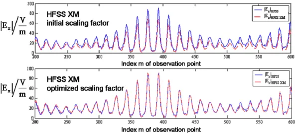
Fig. 7. Comparison of simulated (HFSS) and computed (HFSS XM) electric fields at defined observation points with regard to initial and optimized scaling factor.
3.3 Calculation of the radiation fields on basis of the equiv-alent Huygens sources
The optimization process for calculating the corrected values of the surface current distribution combines these currents to the electromagnetic fields at the defined observation points inside the simulation volume by applying the formalism sum-marised in Eq. (3).
H(rA)=4j kπ ·(m×rA)·C·e−j krA
E(rA)=4ηπ ·(M−m)·|rj k
A|+C
+2MC·e−j krA
C= 1 rA2 ·
1+j k|1r
A|
M= (rA·m)·rA
|rA|2
η=qµ0
ε0 =120π
(3)
The electromagnetic fields are computed directly from an electric dipole momentm=JQ·AQ, whereAQ represents the area of a single triangle used for segmentation of the an-tenna surface, without determining the magnetic vector po-tential and necessary application of the subsequent functions of vector calculus in order to calculate the radiation fields (see Makarov, 2002). The segmented antenna structure con-tains a high number of dipole moments depending on the number of elements necessary for a high quality mesh tri-angulation. Therefore the electromagnetic field in a specific observation pointrAinside the simulation volume is a
super-position of the contributions of allN dipole moments cover-ing the antenna surface.
H(rA)=
N P
n=1
Hn rA−rQ,n
E(rA)= N P
n=1
En rA−rQ,n
(4)
The quality of the calculated radiation fields depends on the quality of the generated mesh and the field solution inside the
simulation volume of HFSS. The interrelation between the surface currents and the electromagnetic fields surrounding the antenna is the basis for the computation of an optimized scaling factor for the current distribution. The iterative pro-cess starts with an initial value ofsfinitial=1. The expressions defined in Eq. (5) are used as a criterion to evaluate the differ-ence between the electric fields based on the field solution of HFSS and the electric fields computed by applying Eqs. (3) and (4) to the surface current distribution. The optimal value of the scaling factor is found for the minimum of the residual error using a Matlab implemented optimizer.
Fx,real,m(sf )=ReEx,H F SS(rm) −ReEx,H F SS XM(rm) 2 Fy,real,m(sf )=ReEy,H F SS(rm) −ReEy,H F SS XM(rm)
2
Fz,real,m(sf )=ReEz,H F SS(rm) −ReEz,H F SS XM(rm) 2
Freal(sf )= 1 M·
M X
m=1
Fx,real,m(sf )+Fy,real,m(sf )+Fz,real,m(sf )
⇒sfoptimal,real=min{Freal(sf ):sf ∈(0,5)}
Fx,imag,m(sf )= I m
Ex,H F SS(rm) −I m
Ex,H F SS XM(rm) 2
Fy,imag,m(sf )=I mEy,H F SS(rm) −I mEy,H F SS XM(rm) 2
Fz,imag,m(sf )=I mEz,H F SS(rm) −I mEz,H F SS XM(rm) 2
Fimag(sf )= 1 M·
M
X
m=1
Fx,imag,m(sf )+Fy,imag,m(sf )+Fz,imag,m(sf )
⇒sfoptimal,imag=minFimag(sf ):sf∈(0,5)
JQ,optimal=sfoptimal,real·ReJQ,initial +j·sfoptimal,imag·I mJQ,initial (5)
132 R. Herschmann et al.: Extended post processing of FEM based simulation results
Fig. 8. Power balance of the spiral antenna; the calculations are performed using different boundary layers in the HFSS simulation.
treatment of the real and imaginary parts generally delivers different optimal scaling factors. An important reference re-garding the quality of the simulator’s field solution is a good agreement betweensfoptimal,real andsfoptimal,imag. There is a risk that an adaption of the electric fields is possible in-side the simulation volume also at an insufficient field con-vergence by the surface currents of the antenna structure, if the number of degrees of freedom of the optimization pro-cess is increased. For instance it is possible to establish sepa-rate scaling factors for the Cartesian components of the elec-tric fields. However the physical significance of the current surface distribution optimized this way is challenged. The chosen implementation of the HFSS XM method avoids this situation. An insufficient convergence of the electromag-netic fields inside the simulation volume results in remaining significant deviations between the HFSS based field compo-nents and the fields extracted from the surface current distri-bution.
3.4 Results and ranges of application
A comparison of the electric fields simulated by HFSS and the electric fields computed on basis of the surface current distribution by HFSS XM in the observation point area in-troduced in Fig. 6 is presented in Fig. 7 at a frequency near the first serial resonance. The two graphics show only an extract of all defined observation points and are restricted to the magnitude of the x-component of the complex electric field vector. Deviations and agreements of the other vector
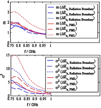
Fig. 9.Statistical evaluation of differences regarding the antenna’s radiated electric fields extracted from HFSS field solution and com-puted from the surface current distribution; the calculations are per-formed using different boundary layers in the HFSS simulation.
R. Herschmann et al.: Extended post processing of FEM based simulation results 133 of the simulated and computed solutions of the electric fields.
The error vectors contain the absolute values of the differ-ences of the magnitudes of the electric fields for every Carte-sian component at the defined M observation points. The low mean average values as well as moderate variances for all three Cartesian components validate the sufficient number of adaptive passes and the very well converged field solution inside the simulation volume.
1Ei(f )=
Ei,1,H F SS(f )
−
Ei,1,H F SS XM(f )
.. .
Ei,m,H F SS(f )
−
Ei,m,H F SS XM(f )
.. .
Ei,M,H F SS(f )
−
Ei,M,H F SS XM(f )
,
i=x, y, z, m=1..M (6) Based on the optimized surface current distribution it is pos-sible to separate ohmic losses of the antenna from radiation losses and select a proper equivalent antenna circuit. Fur-thermore it is possible to compute the electromagnetic fields in arbitrary observation point areas and extract information on polarisation states for example. The implemented method is capable to compute the surface current distribution of ge-ometrical complex shaped antennas for use in UHF-RFID transponder systems.
4 Conclusion
The Matlab implementation of HFSS XM makes the calcu-lation of the surface current distribution of plane antennas as well as the computation of the electromagnetic fields and measures derived from them possible in arbitrary observation points and areas. Furthermore the convergence of the field solution computed by HFSS is checked during the determi-nation of optimized scaling factors for the real and imaginary parts of the antenna’s surface currents. Therefore it improves the capabilities implemented in HFSS already and antenna prototyping for UHF-RFID transponder becomes more so-phisticated. The introduced method is capable to compute the surface current distribution of three dimensional antennas with finite metallization thickness as well as conformal an-tennas. Based on the surface current distribution it is possible to lay out a library containing the geometrical data of param-eterized transponder antennas, the impedance at the feeding point and the related surface current distribution as a function of frequency. Therefore it is not necessary to save the mem-ory intensive HFSS models. The quality of the computed surface current distribution depends on the convergence of the electromagnetic fields inside the simulation volume of HFSS. According to the examinations made in this paper the field convergence necessary for accurate calculation of the surface current distribution requires significant higher num-ber of adaptive passes than a merely impedance convergence at the antenna’s feeding point.
References
Herschmann, R., Camp, M., and Eul, H.: Design und Analyse elek-trisch kleiner Antennen f¨ur den Einsatz in UHF RFID Transpon-der, Adv. Radio Sci., 4, 93–98, 2006,
http://www.adv-radio-sci.net/4/93/2006/.
Makarov, S. N.: Antenna and EM Modeling with MATLAB, John Wiley & Sons Inc., 2002.
Persson, P.-O.: Mesh Generation for Implicit Geometries, in: De-partment of Mathematics, PhD thesis, Massachusetts Institute of Technology, 2005.