Attributing trends in extremely hot days to changes in atmospheric dynamics

(1)

NHESSD

3, 3323–3367, 2015

Extreme hot days and atmospheric

dynamics

J. A. García-Valero et al.

Title Page

Abstract Introduction

Conclusions References

Tables Figures

◭ ◮

Back Close

Full Screen / Esc

Printer-friendly Version Interactive Discussion

Discussion

P

a

per

|

Discussion

P

a

per

|

Discussion

P

a

per

|

Discussion

P

a

per

|

Nat. Hazards Earth Syst. Sci. Discuss., 3, 3323–3367, 2015 www.nat-hazards-earth-syst-sci-discuss.net/3/3323/2015/ doi:10.5194/nhessd-3-3323-2015

This discussion paper is/has been under review for the journal Natural Hazards and Earth System Sciences (NHESS). Please refer to the corresponding final paper in NHESS if available.

Attributing trends in extremely hot days

to changes in atmospheric dynamics

J. A. García-Valero1,2, J. P. Montávez1, J. J. Gómez-Navarro3, and

P. Jiménez-Guerrero1

1

AEMET, Delegación territorial de Murcia, Murcia, Spain

2

Department of Physics, University of Murcia, Murcia, Spain

3

Climate and Environmental Physics, Physics Institute and Oeschger Centre for Climate Change Research, University of Bern, Bern, Switzerland

Received: 7 February 2015 – Accepted: 23 April 2015 – Published: 20 May 2015

Correspondence to: J. P. Montávez (montavez@um.es)

(2)

NHESSD

3, 3323–3367, 2015

dynamics

Title Page

Tables Figures

◭ ◮

Back Close

Full Screen / Esc

Discussion

P

a

per

|

Discussion

P

a

per

|

Discussion

P

a

per

|

Discussion

P

a

per

Abstract

This paper proposes a method that allows the detection of trends in the frequency of extreme events and its attribution to changes in atmospheric dynamics characterized through Circulation Types (CTs). The method is applied to summer Extremely Hot Days (EHD) in Spain during the period 1958–2008. For carrying out this exercise, regional

5

series of daily maximum temperature are derived from the regional dataset Spain02. Eight regions with diﬀ_{erent daily maximum temperature variability are identified. All of} them exhibit important trends in the occurrence of EHDs, especially in inner regions. Links between the probability of EHD occurrence in the regions and CTs have been cal-culated. Furthermore, the consistency of the results to the atmospheric variables used

10

in defining the CTs is analyzed. Sea Level Pressure (SLP), Temperature at 850 hPa Level (T850) and Geopotential Height at 500 hPa Level (Z500) from the ERA40 dataset have been used for the six CT classifications obtained using the variables separately and in diﬀ_{erent combinations of pairs. The optimum choice of large scale variables} depends on the region under consideration, being the combination SLP-T850 the one

15

giving the most suitable characterization for most of them. Finally, an attribution exer-cise of the regional EHD trends to the dynamics is proposed. Results show that the maximum of attributable EHD trends to changes in dynamics in every region is always below 50 %, being even lower than 20 % in those regions with the largest EHD trends, mainly located in the center of the Iberian Peninsula (IP).

20

1 Introduction

Climate suﬀ_{ers changes at di}ﬀ_{erent time scales driven by several external and internal} factors. Human-induced changes in green-house gases, land use, etc., have been es-pecially prominent in the last centuries, modifying the energy balance and therefore in-ducing climate changes (Stocker et al., 2013). The attribution of recent climate change

25

(3)

NHESSD

3, 3323–3367, 2015

dynamics

Title Page

Tables Figures

◭ ◮

Back Close

Full Screen / Esc

Discussion

P

a

per

|

Discussion

P

a

per

|

Discussion

P

a

per

|

Discussion

P

a

per

|

climate and quantify their relative relevance. However, although the main factors per-turbing the climate at global scale have been extensively characterized (Huybers and Curry, 2006; Swingedouw et al., 2011), less exercises with the focus put on regional scales are available (Stott, 2003).

Beyond the average state, the footprint of climate change is manifested through shifts

5

in extreme weather. Along the last years there has been an increasing interest in quan-tifying the role of human and other external influences on climate in specific weather events (Stott, 2003; Zwiers et al., 2011). Therefore, trying to attribute extreme events to climate change at regional scales presents particular challenges for science.

In the last decades Europe has experienced a prominent increase in the

occur-10

rence of extremely warm episodes, especially during summer time (Frich et al., 2002; Klein Tank and Können, 2003; Alexander et al., 2006). The impacts of such events on human health are important, observing high rates of mortality when such extremes oc-cur. Examples of this are the summers of 2003 (Trigo et al., 2005) and 2010 (Dole et al., 2011), when persistent episodes of high maximum temperatures in western and

east-15

ern Europe took place. Several studies show that days exceeding the 95th percentile of the maximum temperature series (extremely hot days) provoke also an increas-ing in mortality especially among the elderly and people with cardiovascular diseases (Díaz-Jiménez et al., 2005). Many works have tried to investigate the causes of these trends, concluding that these are largely influenced by the anthropogenic activity (Stott,

20

2003; Zwiers et al., 2011), being summers like that of 2003 expected to become more frequent under several climate change scenarios (Beniston, 2004). However, extreme events are also driven by unpredictable internal variability. Indeed some authors Dole et al. (2011) argued that the summer of 2010 was the result of the internal variability of the climate system, rather than a clear response to global warming.

25

(4)

NHESSD

3, 3323–3367, 2015

dynamics

Title Page

Tables Figures

◭ ◮

Back Close

Full Screen / Esc

Discussion

P

a

per

|

Discussion

P

a

per

|

Discussion

P

a

per

|

Discussion

P

a

per

on EOFs or CCA. Other studies use CTs (Yiou and Nogaj, 2004; Yiou et al., 2008; Van den Besselaar et al., 2010; Fernández-Montes et al., 2013). These are guided by the results obtained by Corti et al. (1999) who pointed out that recent climate changes can be interpreted in terms of changes in the frequency of occurrence of natural at-mospheric circulation regimes. Some patterns related to anticyclonic and blocking

sit-5

uations favor the development of warm extreme events over Europe (Yiou et al., 2008; Carril et al., 2008; Pfahl, 2014). Therefore, trends in the appearance of these situations can be behind the trends of this kind of events. Many studies using CTs have informed of the increasing observed in the frequency of such patterns since the second half of the past century (Huth, 2001; Kysel´y and Huth, 2006; Philipp et al., 2006; Cony et al.,

10

2010; Bermejo and Ancell, 2009; Fernández-Montes et al., 2013; García-Valero et al., 2012). On the other hand, based on the robustness of the evidence from multiple mod-els, the last IPCC report (Stocker et al., 2013) concludes that it is likely that human influence has altered sea level pressure (SLP) patterns globally since 1951. In that way, climate change induces changes in circulation that can further modify extreme

15

events occurrence.

However, not all studies in literature find strong links between trends in the occur-rence of extreme episodes and trends in the frequency of CTs. Jones and Lister (2009); Bermejo and Ancell (2009); Fernández-Montes et al. (2013) among others, found that trends in extreme temperatures are mainly due to the increase of temperature within

20

the CTs, rather than the increase of the frequency of occurrence of the CTs. This could suggest that trends in extremes can be in addition linked to other forcings such as: global warming, teleconnection phenomena (El Kenawy et al., 2012; Della-Marta et al., 2007), dryness of soil, increase of the SST, etc. Discrepancies in relating both kind of trends might be provoked by the way CT classifications are built. In general,

classifica-25

(5)

NHESSD

3, 3323–3367, 2015

dynamics

Title Page

Tables Figures

◭ ◮

Back Close

Full Screen / Esc

Discussion

P

a

per

|

Discussion

P

a

per

|

Discussion

P

a

per

|

Discussion

P

a

per

|

García-Valero et al., 2012). In addition, the atmospheric patterns associated with ex-treme events represent a small number of days in relation to total of days clustered, therefore they could not be well represented in the CT classifications performed until now, and their trends may not be reliable.

Another aspect to consider is how trends in extremes of temperature are obtained.

5

Although most studies in literature calculate such trends from local stations, this is prob-lematic since part of their variability can be driven by local factors, hiding in part the signal imposed by the footprint of the large-scale dynamics at regional scales. There-fore, we use regional instead of local series, with the aim of highlighting the explanation of the response to dynamic conditions (Lorente-Plazas et al., 2014).

10

This study is applied over the IP because of several reasons. First, the IP has expe-rienced a large increase in the summer maximum temperatures in the last and current century (Brunet et al., 2007; Rodríguez-Puebla et al., 2010; Hertig et al., 2010; El Ke-nawy et al., 2011). Second, atmospheric systems impact in a very diﬀ_{erent way over} the territory because of its complex topography, provoking an important spatial

vari-15

ability (Font-Tullot, 2000). On the other hand, in the last years diﬀ_{erent dense datasets} have been developed for the IP favoring the availability of necessary data for this kind of studies (Herrera et al., 2010; Gómez-Navarro et al., 2012a) Finally, The IP has been identified as one of the areas more sensitive to climate change and especially in sum-mer, either by changes provoked by external forcings (Gómez-Navarro et al., 2012b),

20

or by anthropogenic forcing (Giorgi, 2006).

In this context, the present analysis aims at quantifying changes in the observed re-gional EHD trends and their relation with atmospheric dynamics. This contribution is organized as follows: Sect. 2 describes the databases used for maximum temperature and atmospheric fields; in Sect. 3 the regionalization procedure of the maximum

tem-25

(6)

NHESSD

3, 3323–3367, 2015

dynamics

Title Page

Tables Figures

◭ ◮

Back Close

Full Screen / Esc

Discussion

P

a

per

|

Discussion

P

a

per

|

Discussion

P

a

per

|

Discussion

P

a

per

links, and the attribution of the EHD trends to the changes of the CTs are explained in Sect. 5. Finally, main conclusions and discussions are in Sect. 6.

2 Data

2.1 Surface temperature data

Several high resolution climate databases for the IP (Herrera et al., 2010) or including

5

it (Caesar et al., 2006; Haylock et al., 2008) have been developed during the last years. These databases have been built by interpolation techniques applied to, in principle, a dense observation network. Although generally reliable, these databases present some known inconsistencies (Gómez-Navarro et al., 2012a) due to diﬀ_{erences in the} raw observational series, the interpolation method, or the diﬀ_{erent quality controls}

ap-10

plied to the data.

In this work, we use the maximum daily temperature obtained from Spain02 (Her-rera et al., 2010) grid dataset, due to the larger number of stations used compared to other similar products available. The large spatial resolution over mainland Spain and Balearic islands (0.2◦

×0.2◦), together with the length of the period (1951–2008),

en-15

sures a suﬃ_{cient spatial and temporal coverage over the study area. Since the work} focus on extremely hot days, only dates between 16 June and 15 September are con-sidered.

2.2 Large scale atmospheric data

The data for characterizing the structure of the atmosphere consist of daily fields at

20

12:00 UTC of Sea Level Pressure (SLP), Temperature at 850 hPa (T850) and Geopo-tential Height at 500 hPa level (Z500) extracted from the ERA40 reanalysis (1958– 2002) (Uppala et al., 2005) and ECMWF analysis (2003–2008). The maximum com-mon resolution (1.125◦_{) is used for the period 1958–2008. The variables considered}

(7)

NHESSD

3, 3323–3367, 2015

dynamics

Title Page

Tables Figures

◭ ◮

Back Close

Full Screen / Esc

Discussion

P

a

per

|

Discussion

P

a

per

|

Discussion

P

a

per

|

Discussion

P

a

per

|

to extreme heat events. In this context, SLP oﬀ_{ers information about fluxes at low} lev-els, hence informing about the area of provenance of the air mass reaching a given region. T850 informs about the temperature at low atmospheric levels, tightly related to surface temperature (Brands et al., 2011). Finally, Z500 provides a global vision of the mean atmospheric state. Furthermore, it provides some insight about the overall trough

5

and ridge patterns over the study area, indicating large advection and subsidence in the atmosphere (Sheridan et al., 2012).

3 Regional series and EHD

This section describes the methodology to identify a set of regions that cluster local series with similar temporal variability of the summer maximum temperature. Spatially

10

averaged regional series filter out local factors and provide a robust characterization of extreme situations aff_{ecting the di}ff_{erent regions, as well as simplify the exposure of} the diff_{erent behaviors.}

3.1 Clustering procedure

The procedure applied is similar to that employed by Jiménez et al. (2008). First, a

Prin-15

cipal Component Analysis (Storch and Zwiers, 1999) in S-mode is applied to the cor-relation matrix obtained from daily anomalies. Only the three first EOFs following the scree plot test (Cattell, 1966) were retained, explaining more than 80 % of total vari-ance. Second a two step clustering method is applied to the loadings of each grid point in the retained EOFs. The Ward algorithm (Ward, 1963) is employed for obtaining

20

(8)

NHESSD

3, 3323–3367, 2015

dynamics

Title Page

Tables Figures

◭ ◮

Back Close

Full Screen / Esc

Discussion

P

a

per

|

Discussion

P

a

per

|

Discussion

P

a

per

|

Discussion

P

a

per

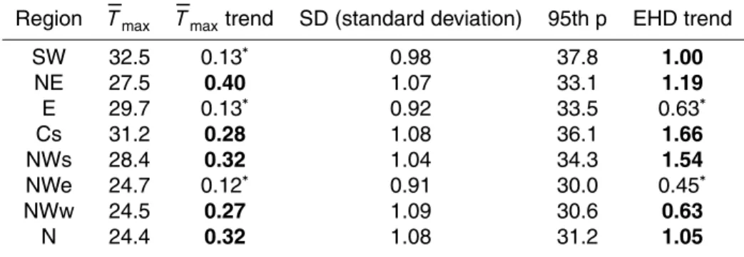
3.2 Regions

The aim of this study is not to perform an exhaustive analysis of the regions, but rather to use the regional series as a tool for achieving the final target, so only some aspects related to the time variability are presented below. Figure 1 shows the eight regions obtained by the clustering procedure. The name of regions has been established

ac-5

cording to their geographical locations: SW, NE, E, Cs, NWs, NWe, NWw and N. Re-gional series have been constructed by averaging the time series of all the grid points belonging to the same region. Table 1 (first four columns) shows some statistics of the regional series: mean, trend, standard deviation and 95th percentile. A meridional gra-dient of mean and percentile values is observed, being the warmest regions located in

10

the southern half of the country (SW and Cs). In addition, distance to the sea is an-other factor influencing the maximum temperature spatial distribution. Inner regions are warmer and have higher standard deviation. Some examples are NWs and NE regions in the northern half, and Cs in the South.

The temporal variability of the regional series is analysed in Fig. 2, that shows the

15

seasonal mean series (solid black curve). As previously pointed out by Brunet et al. (2007) for the IP, as well as for other further Mediterranean regions Burić_{et al. (2014),} two periods with diﬀ_{erent behaviour stands out in all regions. The first lies between} 1951 and 1977, when temperatures dropped significantly, being 1977 the coldest year for most regions. The second period (1978–2007) is characterized by a significant rise

20

of the maximum temperatures. The 90’s decade was especially warm, occurring the hottest year for most regions. In particular, 1994 was the hottest for eastern (NE, E and Cs), 1991 for western (SW and NWs) and 1990 for northern regions. During the last decade, it is observed changes of the standard deviation of the regional series, de-creasing over the central, southern and eastern regions, whereas inde-creasing in

north-25

(9)

NHESSD

3, 3323–3367, 2015

dynamics

Title Page

Tables Figures

◭ ◮

Back Close

Full Screen / Esc

Discussion

P

a

per

|

Discussion

P

a

per

|

Discussion

P

a

per

|

Discussion

P

a

per

|

3.3 Extremely hot days

In this work, a day is defined as Extremely Hot Day (EHD) when the maximum regional temperature series exceeds its 95th percentile in any of the regional series (values in the 5th column of Table 1). A total of 863 EHDs were identified for this study.

Some aspects related to annual variability of the regional EHDs series, as well as

5

a comparison of simultaneous occurrence of EHD among the diﬀ_{erent regions, have} been analyzed. Annual number of EHD for the various regions are shown by vertical bars in Fig. 2. All regions show a noticeable increase in EHDs since the 90s. This finding agrees with those obtained for the IP by Brunet et al. (2007) and Fernández-Montes et al. (2013) as well as for Europe by Klein Tank and Können (2003). Thus,

10

positive and significant trends are obtained in all regions (Table 1), being the trends larger in the inner regions (NE, Cs, NWs). It is noteworthy that the year with the highest number of EHDs depends on the region. The year with the maximum number of EHDs is 2003 for the northern regions (N, NWe, NWs and NE). This is not surprising since it coincides with the extraordinary heat wave occurred in many places of western Europe

15

(Beniston, 2004; Trigo et al., 2005). Furthermore, this event is also characterized by a great persistence. NE, N, NWe, NWs and SW regions suﬀ_{ered EHD persistences up} to 10 days (NE, N, NWe, NWs) and 16 days (SW). The maximum number of EHDs took place in the early 90s in the rest of the regions. Curiously, in the E region, the maximum of EHD occurred in two consecutive years (1958 and 1959).

20

A trend analysis of the seasonal EHD series (6th column of Table 1) was performed using the Sen’s algorithm (Sen, 1968) using the period 1958–2008. All regions have positive and significant trends at 95 % (significances obtained by the Mann–Kendall test), but E and NWe that are significant at 90 %. The inner regions show the larger trends (Cs, NWs and NE), a similar warming pattern to that obtained by Bermejo and

25

(10)

NHESSD

3, 3323–3367, 2015

dynamics

Title Page

Tables Figures

◭ ◮

Back Close

Full Screen / Esc

Discussion

P

a

per

|

Discussion

P

a

per

|

Discussion

P

a

per

|

Discussion

P

a

per

One important aspect to study is how diﬀ_{erent is the behavior of EHD among the} diﬀ_{erent regions. Table 2 shows the probability of having simultaneous occurrences of} EHDs between pairs of regions. The diagonal values are the probability of occurrence of an EHD in only one region. The region which has the most independent behavior is E region (40 %), while NWs shares many episodes with many other regions (5 %). The

5

lowest probability of simultaneous EHD occurrences is for E and NWs (15 %), while the largest is for NWs and SW (62 %). In general, there are important regional diﬀ_erences, which points to the conclusion that a given large atmospheric pattern should provoke diﬀ_{erent behaviors along the various regions.}

4 Characterization of EHDs circulation types

10

As discussed above, the links between EHD occurrences and CTs can be hampered by the low signal-to-noise ratio that most CT classifications present, since they are usually obtained considering all days within a long extended period of time. For our purpose, it is more reasonable to obtain the CT classification using only extreme days, i.e, to characterize the atmospheric circulation that drives these extreme situations. On the

15

other hand, such links could be sensitive to the large scale atmospheric variables used for the CT classification. Hence, in this section we construct the CTs using only the days classified as EHD and diﬀ_{erent combinations of large scale atmospheric variables and} analyze the links between EHD occurrence and the CTs, trying to identify the most suitable set of atmospheric variables for characterizing the EHDs.

20

4.1 CT Classification procedure

The clustering method followed for the CT classifications is the same employed in Ky-sel´y and Huth (2006) and García-Valero et al. (2012). It bases on a two step procedure. First a PC-ModeT clustering is applied to the Rotated Empirical Orthogonal Functions (REOF) obtained from the retained EOFs of the T-Mode. A scree plot test (Cattell,

(11)

NHESSD

3, 3323–3367, 2015

dynamics

Title Page

Tables Figures

◭ ◮

Back Close

Full Screen / Esc

Discussion

P

a

per

|

Discussion

P

a

per

|

Discussion

P

a

per

|

Discussion

P

a

per

|

1966) is used to select the number of retained modes. This step provides the centroids (composites of the anomalies of each cluster) that are projected over the PCs retained in the S-mode. Then, this projections are used as initial seeds to initialize the second step: a K-means clustering.

The input for the clustering procedure consist of the atmospheric situations for the

5

784 days classified as EHD within the period (1958–2008). The spatial window consid-ered for the classifications covers enterely the IP (35–45◦_{N and 10}◦_W–6◦_{E) and it is}

formed by 150 grid points. This configuration is identical to that used in García-Valero et al. (2012). A larger spatial window is used to represent the centroids.

For the identification of the optimal atmospheric variables in representing the EHDs,

10

six diﬀ_{erent CTs classifications are obtained. Three of them consider the atmospheric} variables individually (SLP, T850 and Z500). In this case, each classification is formed by six clusters (being this number the double of the retained PCs, García-Valero et al., 2012). The other three classifications consider all possible pairs of variables: SLP-T850 (Fig. 3), SLP-Z500 (Fig. 5) and Z500-T850 (Fig. 4), and they are formed by eight (four

15

retained PCs) clusters each one. In all cases the retained PCs explains nearly the 90 % of the total variance.

4.2 Evaluation of the CT classifications for EHD description

In the ensemble of the EHDs clustered in the six obtained CTs classifications, there are days that are extremes for one or various regions but not for the other regions, and vice

20

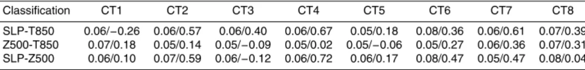
versa. Therefore, within a given CT classification, there are some CTs more related to the occurrence of EHDs in some regions. An important question is whether for a given region there is, among the six classifications, anyone that discriminates better the EHD occurrence. In order to address this question an eﬀ_{ectiveness index (EI) is defined.} This index is calculated as the ratio between the number of EHD occurrences and non

25

(12)

NHESSD

3, 3323–3367, 2015

dynamics

Title Page

Tables Figures

◭ ◮

Back Close

Full Screen / Esc

Discussion

P

a

per

|

Discussion

P

a

per

|

Discussion

P

a

per

|

Discussion

P

a

per

deviation and range of the EIs are the largest, since it separates better the most from the less influential CTs.

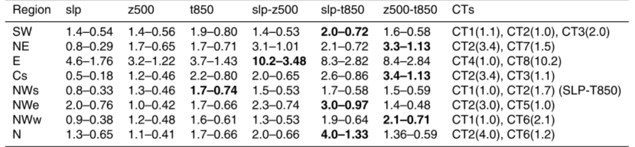
Table 3 shows the range and standard deviation (range-sd) obtained for all the re-gions and CT classifications. Last column shows the best (highlighted in black) CT classification, as well as their extreme CTs for each region. Results indicate that two

5

synoptic variables characterize better the EHDs for most regions. Z500-T850 is the best one for NE, NWw and Cs (inner-eastern regions and northwestern). SLP-Z500 characterizes better E region. SLP-T850 is the best for SW, NWe and N (western and northern regions). T850 classification is the best for the NWs region. However, in this area SLP-T850 perform quite similar. Hence, and for the shake of clarity in the

analy-10

sis, SLP-T850 has been considered as the best classification in this case. Figures 3–5 show all the CTs (contours) of the best CT classifications and the eﬃ_{ciencies for each} region (shaded). Eﬃ_{ciency is defined as the conditional probability of having an EHD in} a region under a given CT. Another interesting parameter is the contribution of a given CT to the occurrence of the EHDs in a given region. The contribution is assessed by

15

calculating the ratio between the number of observed EHDs under a CT and the total EHDs observed in a region. Tables 4 and 5 depict the eﬃ_{ciencies and contributions} values.

The eﬃ_{ciency patterns are quite similar for the three CT classifications. However,} for each region the eﬃ_{ciency is larger for the classification that gives larger spreads}

20

in the EI index (Table 3). Some examples follow. The effi_{ciency pattern related to CT8} is equivalent in all classifications and shows high effi_{ciency over the E region. The} effi_{ciency is larger for the SLP-Z500 classification which has the largest EI index for E} region. Similar results are found for SLP-T850, CT6-Z500-T850 (best) and CT5-SLP-Z500 in the NWw region, and for CT3-SLP-T850 (best), CT3-Z500-T850 and

CT1-25

(13)

NHESSD

3, 3323–3367, 2015

dynamics

Title Page

Tables Figures

◭ ◮

Back Close

Full Screen / Esc

Discussion

P

a

per

|

Discussion

P

a

per

|

Discussion

P

a

per

|

Discussion

P

a

per

|

shown). This highlights the need of studies on the sensitivity of the CT classification to the atmospheric variables employed.

The comparison of the atmospheric situations among the diﬀ_{erent classification} as-sociated with similar spatial eﬃ_{ciency patterns, enables to draw conclusions about the} main drivers related to the EHD occurrences. Regarding the T850 variable, the regional

5

eﬃ_{ciency shows the highest values at regions where temperatures are near and above} 20◦_{C. This feature is very common in many CTs of the di}_ﬀ_{erent classifications such}

as the CTs-2/3/4/6/8 of SLP-T850 and the CTs-1/2/3/4/5/7/8 of the Z500-T850 classi-fication. The wind provenance, inferred considering the SLP field, is also an important factor contributing the occurrence of EHDs in some regions, because of the warm

ad-10

vection over specific regions. Many CTs are related to situations when wind blows from inner towards coastal areas, provoking the highest eﬃ_{ciencies in the latter. The inner IP} regions are high land plateau areas where the highest temperatures are observed (see Table 1). When wind blows from this area towards the sea along valleys, air is adiabat-ically compressed causing an important warming at low land regions. Some examples

15

of these situations can be identified in the classifications by analyzing the eﬃ_ciencies and contributions of some CTs. Five regions are mainly aﬀ_{ected by this. NWw,} espe-cially when wind blows from the East because of the presence of High Pressures over western Europe (CT5 of SLP-T850 and SLP-Z500). SW in northeastern winds condi-tions (CTs-1/3 of SLP-T850 and CT1 of SLP-Z500) as result of the presence of high

20

pressure over the Mediterranean and relative low pressures over the southwest of the IP. The E region under strong western zonal wind (CT8 of SLP-T850 and SLP-Z500), induced by the location of High/Low pressures over the Atlantic/Mediterranean. The NE and N regions in southwestern winds situations (CT6 of SLP-T850 and SLP-Z500). Conversely, CTs with weak SLP gradients (stagnant situations linked to thermal lows)

25

(14)

NHESSD

3, 3323–3367, 2015

dynamics

Title Page

Tables Figures

◭ ◮

Back Close

Full Screen / Esc

Discussion

P

a

per

|

Discussion

P

a

per

|

Discussion

P

a

per

|

Discussion

P

a

per

over the IP. Regions with the highest eﬃ_{ciencies are located to the west of ridge axis,} where atmosphere presents a large stability and warm advection. The eﬃ_{ciency and} contribution is only important in the E region when zonal wind at 500 hPa is strong (CT-5/8 of Z500-T850 and CT-8 of SLP-Z500). This pattern usually takes place when hot episodes over the IP are ending up. The analysis of the CT transitions (not shown) for

5

consecutive EHD episodes reinforces this result. The hottest areas travel from western to eastern regions, following the ridge movement.

5 Linking EHD trends to CTs

Positive and significant EHD trends appear across all regions (Sect. 3.2). Thus, an interesting question is whether there exists any relation between these trends and the

10

changes in the CTs frequency appearance.

5.1 Allocation method

The CTs driving the EHD occurrence as well as their eﬃ_{ciencies over each region,} were characterized above. This was made using only EHD days. The analysis shows that most patterns do not always lead to an EHD (Table 4) in a given region. Therefore,

15

in order to find the links between EHD and CTs changes, it is convenient to use all days, (Table 4). This section presents the methodology used to allocate those unused days to the obtained CT classifications.

Each centroid is the result of a set of similar atmospheric conditions. The CTs rep-resented are the mean value of this set of atmospheric situations. However, there is

20

some dispersion inside each group. To allocate an atmospheric situation into a Circula-tion Type means to find the populaCircula-tion where such situaCircula-tion fits better. For this task the election of some metrics is fundamental. Two metrics have been used for assigning the days initially not considered to each of the obtained CT: the Spearman correlation and the Euclidean distance. The former measures the spatial similarity of two fields (Hofer

(15)

NHESSD

3, 3323–3367, 2015

dynamics

Title Page

Tables Figures

◭ ◮

Back Close

Full Screen / Esc

Discussion

P

a

per

|

Discussion

P

a

per

|

Discussion

P

a

per

|

Discussion

P

a

per

|

et al., 2012; Vautard and Yiou, 2009) whereas the latter evaluates the diﬀ_{erences in} the intensity of patterns (Fettweis et al., 2011). Both metrics are relevant and comple-mentary (Nogaj et al., 2007; Fettweis et al., 2011). The population of a given CT will be characterized by the distribution of the distances to and correlations with the centroid. A criterium to allocate a situation in a given CT is that the distance to/correlation with

5

the centroid be lower/higher than some given thresholds. The most objective election of thresholds is the maximum distance and the minimum correlation of the population for each CT. Table 6 shows the thresholds chosen for all CTs.

Prior to the allocation process, all days and centroids are standardized at each grid point. A day is allocated in a given CT when both, distance and correlation, are lower

10

and higher, respectively, than a defined threshold value for each one. Days that are not allocated in any CT are assigned to a new group (unclassified group, CT9) (Seu-bert et al., 2014). It is possible to find atmospheric situations that can be assigned to several clusters. In these cases, they are allocated to the nearest cluster considering the euclidean distance. The use of the euclidean distance as definitive criteria obeys

15

mainly to the lower variance of the distance population.

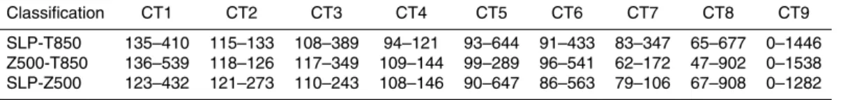
5.2 Results of the allocation

Table 8 shows the number of days belonging to the diﬀ_{erent CTs before/after the} al-location process. Approximately 70 % of the days for all classifications are assigned, whereas the rest are allocated into the unclassified cluster (CT9), being Z500-T850

20

(SLP-Z500) the one with more (least) unclassified days (33 vs. 28 %). There is a large variability in the increase of the days belonging to the diﬀ_{erent CTs. CT1, CT6 and CT8} have the largest increase (10 times) in all classifications, whereas others like CT2/4-SLP-T850 and CT2/4-Z500-T850 present small changes (less than 20 % of the initial clustered days).

25

(16)

NHESSD

3, 3323–3367, 2015

dynamics

Title Page

Tables Figures

◭ ◮

Back Close

Full Screen / Esc

Discussion

P

a

per

|

Discussion

P

a

per

|

Discussion

P

a

per

|

Discussion

P

a

per

in all cases. Z500-T850 classification has the best quality, producing even an increase in the quality of clusters after the allocation. The quality of the other classifications worsen slightly after the allocation, being the SLP-T850 classification slightly better than the SLP-Z500. On the other hand, the quality of all classifications after the alloca-tion are of the same order than other classificaalloca-tions (summer) such as those obtained

5

in Philipp et al. (2006) (ECV<_{40 %) and García-Valero et al. (2012) (47.2 %). These}

results support the suitability of the criterion used for defining the thresholds in the al-location method, making not necessary the choice of others more restrictive and not exempts from subjectivity.

It is instructive to explore the consequences on the properties of the groups after

10

applying the allocation procedure. One consequence of the larger number of classified days, is the decrease in the effi_{ciency of the CTs (see Table 4). Obviously, the lower} increase of number of days, the lesser decrease of the effi_{ciency. This e}ff_{ect stands} out in CT-2/4 for the SLP-T850 and Z500-T850 classifications, which have the highest effi_{ciencies in most regions. The shape of the population distribution of the distances}

15

and correlation in each CT can be also aff_{ected. The e}ff_{ect of the allocation process} is to include new days located further from the centroid. Nevertheless, a small number of clusters hardly change the populations after the assignation (CT2-4-SLP-T850, CT-2/4-Z500-T850 and CT-4/7-SLP-Z500) which are coincident with the ones with higher effi_{ciency. Figure 6 shows two examples of the correlation histograms before and after}

20

the allocation process and their overlap (top) and the empirical cumulative distribution function (bottom). Left/right panels show an example of great/small changes in popu-lation.

The most eﬃ_{cient CTs for several regions are the patterns better identified in the} characterization step (with more restrictive thresholds, Table 6) and therefore are less

25

(17)

NHESSD

3, 3323–3367, 2015

dynamics

Title Page

Tables Figures

◭ ◮

Back Close

Full Screen / Esc

Discussion

P

a

per

|

Discussion

P

a

per

|

Discussion

P

a

per

|

Discussion

P

a

per

|

the E and NWw regions, which are now better characterized by the SLP-T850 classifi-cation.

Seasonal trends in the frequency of the CTs are also aﬀ_{ected by the allocation.} Table 9 shows the trends before/after the allocation obtained by using the Sen trend estimator as well as their statistical significances considering the Mann–Kendall test.

5

Nevertheless, those CTs with higher eﬃ_{ciency in the EHD occurrence remains almost} unchanged, CT2 for all classifications.

Attending to these results, and considering all classifications, significant trends in CTs frequency contribute more to a higher frequency of EHDs in northern regions, mainly at N and NE.

10

5.3 Attribution of trends

Temperature changes can be linked to several factors, being one of them the changes in the frequency of the CTs. Trends in the EHDs could be considered also as an indica-tor of temperature changes. In this subsection, a simple attribution model of the EHDs trends to the trends in the CTs frequency appearance is presented.

15

The trend in EHD in a given regionTr can be written as the sum of two terms:

Tr=T_cr+T_or (1)

whereT_cris the trend attributable to changes in atmospheric circulation andT_orthe trend related to other factors. Now,T_cr _{can be described as a linear function of the changes}

in the frequency of the CTs. We propose the simple model:

20

T_cr=

n

X

i=1

T_iǫr

i (2)

where the subscripti _{denotes the CT number, from 1 to} n_{(the number of CTs),}T_i _is

the frequency trend of the CTi andǫ

r

(18)

NHESSD

3, 3323–3367, 2015

dynamics

Title Page

Tables Figures

◭ ◮

Back Close

Full Screen / Esc

Discussion

P

a

per

|

Discussion

P

a

per

|

Discussion

P

a

per

|

Discussion

P

a

per

Using this simple model T_cr _{can be calculated for all regions using the CT}

classifi-cations obtained above. The results are summarized in Table 10. The fourth column depicts the observed regional trend. The trends reproduced by this simple model are smaller than the observed, also appearing an important variability among the regions. For most regions the reproduced trends strongly depends on the CT classification, but

5

few diﬀ_{erences appears in the SW and NWw regions. In general terms, the Z500-T850} classification obtains the biggest reproduced trends but for NWw. Using this classifica-tion a fracclassifica-tion between 40–50 % of the observed trends is attributed in the E, NE, NWe and N regions, about 20 % in the western and southern regions (SW, Cs and NWs) and hardly 14 % in the NWw to changes in the atmospheric dynamics.

10

5.4 E_fficiency of within type variations

Previous works analyze the Within Type (WT) variations of the maximum and minimum temperatures inside the CTs (Fernández-Montes et al., 2013; Bermejo and Ancell, 2009; Jacobeit et al., 2009). They show that many CTs warms during the second half of the past century, observing a higher warming for minimum than for maximum

tem-15

peratures for the Iberian Peninsula. WT variations are a signal of the changes in the physical links between dynamics and regional variability that at the same time could be modulated by other mechanisms (soil moisture, sea surface temperature, etc.). Thus, in order to evaluate the stability of the relationships between the CTs and EHDs, the possible existence of WT variations in the eﬃ_{ciency of the CTs in each region has been}

20

analyzed. For the analysis the moving average eﬃ_{ciency series (31 year) of the best} classification for each region has been calculated (Fig. 7).

In general, the CTs related to the highest eﬃ_{ciencies in each region increase its} eﬃ_{ciency by 10 % along the study period (1958–2008). This is the case of CT2 in} the regions Cs, NWs, NWe, NWw and N, and CT4 in the E region. There are some

25

(19)

NHESSD

3, 3323–3367, 2015

dynamics

Title Page

Tables Figures

◭ ◮

Back Close

Full Screen / Esc

Discussion

P

a

per

|

Discussion

P

a

per

|

Discussion

P

a

per

|

Discussion

P

a

per

|

However, CT4 shows an eﬃ_{ciency decrease in the northern regions (NWw, NWe and} N), although the eﬃ_{ciency increases in the E region.}

NE region is the least aﬀ_{ected by WT variations. Only CT1 increases its e}ﬃ_ciency, but it is low over the region. Other authors (Bermejo and Ancell, 2009) found that this area has experienced the highest trends in mean maximum temperatures of the IP,

5

attributing such trends to WT variations.

One of the reasons of the eﬃ_{ciency growth of some CTs can be the increase in} the persistence. Thus, the higher the persistence of a CT leading EHD, the higher the temperature rises. Hence, the persistence of hot situations favors the development of land-atmosphere positive feedbacks that enhance the air temperature (Jerez et al.,

10

2012; Seneviratne et al., 2010). To evaluate this possible influence, the correlation be-tween the de-trended seasonal frequency series and the mean seasonal persistence series of the CTs with the most important WT have been calculated. Results show pos-itive and significant correlations, between 0.6 and 0.7, which support the influence of the persistence on the eﬃ_{ciency rise. In addition, the decline of soil moisture observed}

15

over the IP since 1970s (Sousa et al., 2011) can be an additional factor contributing to this feedback process.

6 Conclusions and discussions

This study characterizes the Circulation Types leading summer EHDs occurrence over Spain, defining the EHDs as those when 95th percentile of the maximum daily

temper-20

ature series is exceeded. For that, a regionalization of maximum daily temperatures in summer have been carried out. The analysis of regional series shows the existence of positive trends in the EHD seasonal frequency in all regions. For the characterization of the CTs three atmospheric variables, SLP, T850 and Z500, have been considered for building six CT classifications, three for the variables used individually and other three

25

(20)

NHESSD

3, 3323–3367, 2015

dynamics

Title Page

Tables Figures

◭ ◮

Back Close

Full Screen / Esc

Discussion

P

a

per

|

Discussion

P

a

per

|

Discussion

P

a

per

|

Discussion

P

a

per

the links between the CTs and the occurrence of EHD in the regions have been evalu-ated through the effi_{ciency coe}ffi_{cients. These e}ffi_{ciencies and the trends observed in} the frequency of CTs have been used for proposing an method for trying to attribute the EHD trends observed in the diff_{erent regions to changes in the atmospheric dynamics.} Finally, the stability of links have been studied. The main conclusions are summarized

5

below.

– Eight regions with diﬀ_{erent time variability of daily maximum temperatures are} identified. Positive an significant trends in EHDs are found across most regions. Generally, such trends are larger in central and northern regions, and lower at SE and NWe regions.

10

– When a CT classification is designed for describing the EHDs occurrences, the election of the most suitable combination of atmospheric variables become of major relevance. This study finds that classifications using combinations of two atmospheric variables generally perform better than those using only one. In the case of the studied area, SLP-T850 characterizes better the EHD occurrences for

15

most regions. However, other combinations such as Z500-T850 has better results in the Cs, NE and NWw regions, and SLP-Z500 in the E region.

– For the characterization of atmospheric patterns driving extreme events, it is con-venient to use only days classified as extremes. This increases the signal-to-noise ratio of the CT classifications against those obtained using all situations. However,

20

this classifications have to be extended to accommodate the rest of days initially not defined as extremes when the aiming is to perform an attribution exercise as the proposed here. The allocating method used produces extended classifica-tions of quality. The extended CT classification based on Z500-T850 has the best quality whereas the SLP-Z500 one is the worst.

25

(21)

NHESSD

3, 3323–3367, 2015

dynamics

Title Page

Tables Figures

◭ ◮

Back Close

Full Screen / Esc

Discussion

P

a

per

|

Discussion

P

a

per

|

Discussion

P

a

per

|

Discussion

P

a

per

|

and Ancell, 2009). Such trends depend on the atmospheric variables used for the classification, occurring the largest trends in the classification of the best qual-ity (Z500-T850). CT 2 of the Z500-T850 and SLP-T850 classifications have the largest trends. This atmospheric pattern is associated with high occurrence of EHDs in most regions simultaneously, especially in the central and northern

re-5

gions.

– Part of the EHD trends observed in some regions can be attributed to changes in the CT frequencies alone. However, trends reproduced by the attribution method are in all cases lower than the observational ones, indicating that part of the trend has to be attributed to other factors. The attributed trends have a great

depen-10

dence on the region, as well as on the CT classification. Thus, the best quality classification, Z500-T850, is able to attribute the larger part of the EHD observed trends for most regions but for NWs. Considering this classification a fraction be-tween 30–50 % of the observed trends is attributed in the E, NE, NWe and N regions, about 20 % in the western and southern regions (SW, Cs and NWs) and

15

hardly 14 % in the NWw.

– Some of the most influential CTs on leading EHDs in the diff_{erent regions present} WT variations in relation to its effi_{ciency, but for NE. Approximately the most e}ffi -cient CTs have increased their effi_{ciencies by 10 % during the study period, being} accompanied this variation by an increase of the persistence of such CTs.

20

The attribution exercise reveals that the trends observed can be only partially at-tributed to changes in the atmospheric dynamics, and that they have an important regional component. This would suggest that the factors involved in the EHD trends, at least in the Iberian Peninsula, tends to be positive, i.e. changes in factors such as global warming, soil–atmosphere feedbacks or changes of surface properties leads

25

(22)

NHESSD

3, 3323–3367, 2015

dynamics

Title Page

Tables Figures

◭ ◮

Back Close

Full Screen / Esc

Discussion

P

a

per

|

Discussion

P

a

per

|

Discussion

P

a

per

|

Discussion

P

a

per

soil moisture that enhances the positive land-atmospheric feedback. This also support the WT variations mentioned above.

The relationship between EHDs and CTs, as well as the allocation methodology presented, can be used as a base for a statistical downscaling method that enables EHD forecast, as well as in regional climate change experiments. In the latter case,

5

WT variations could be a drawback, however in this particular case the changes in the eﬃ_{ciencies are small and therefore, the uncertainty related to WT could be less than} the one related to other factors such as the global circulation models or the scenario.

The general methodology applied here could be extended to other variables or types of events such as floods, droughts, heat waves, cold events, etc. The robustness of

10

the regional series as well as the identification of the best large-scale atmospheric variables characterizing such events could be of crucial importance when trying to relate regional extreme behavior to atmospheric dynamics. In addition, an extension of this methodology can be applied to obtain regional climate change escenarios of extreme events.

15

Acknowledgements. This study was supported by the Spanish governement and the Fondo

Europeo de Desarrollo Regional (FEDER) through the projects SPEQTRES (CGL2011-29672-C02-02) and REPAIR (CGL2014-59677-R). P. Jimenez-Guerrero thanks the Ramon y Cajal Program of the Spanish Ministry of Science and Innovation. The authors also thank to Sonia Fernandez-Montes and the anonymous reviewers for their constructive suggestions.

20

References

Alexander, L., Zhang, X., Peterson, T., Caesar, J., Gleason, B., Klein Tank, A., Haylock, M.,

Collins, D., Trewin, B., Rahimzadeh, F., Tagipour, A., Rupa, K., Revadekar, J., Griﬃ_ths,

G., Vincent, L., Stephenson, D. B., Burn, J., Aguilar, E., Brunet, M., Taylor, M., New, M., Zhai, P., Rusticucci, M., and Vazquez-Aguirre, J. L.: Global observed changes in daily

cli-25

(23)

NHESSD

3, 3323–3367, 2015

dynamics

Title Page

Tables Figures

◭ ◮

Back Close

Full Screen / Esc

Discussion

P

a

per

|

Discussion

P

a

per

|

Discussion

P

a

per

|

Discussion

P

a

per

|

Beniston, M.: The 2003 heat wave in Europe: a shape of things to come?, An analysis based on Swiss climatological data and model simulations, Geophys. Res. Lett., 31, L02202, doi:10.1029/2003GL018857, 2004. 3325, 3331

Bermejo, M. and Ancell, R.: Observed changes in extreme temperatures over Spain during 1957–2002, using Weather Types, Revista de Climatología, 9, 45–61, 2009. 3326, 3331,

5

3340, 3341, 3342

Brands, S., Taboada, J., Cofino, A., Schneider, C., Brands, S., Taboada, J. J., Cofiño, A. S., Sauter, T., and Schneider, C.: Statistical downscaling of daily temperatures in the NW Iberian Peninsula from global climate models: validation and future scenarios, Clim. Res., 48, 163– 176, 2011. 3329

10

Brunet, M., Jones, P., Sigró, J., Saladié, O., Aguilar, E., Moberg, A., Della-Marta, P., Lis-ter, D., Walther, A., and López, D.: Temporal and spatial temperature variability and change over Spain during 1850–2005, J. Geophys. Res., 112, D12117, doi:10.1029/2006JD008249, 2007. 3327, 3330, 3331

Burić_{, D., Lukovi}ć_{, J., Duci}ć_{, V., Dragojlovi}ć_{, J., and Doderovi}ć_{, M.: Recent trends in daily}

tem-15

perature extremes over southern Montenegro (1951–2010), Nat. Hazards Earth Syst. Sci., 14, 67–72, doi:10.5194/nhess-14-67-2014, 2014. 3330

Caesar, J., Alexander, L., and Vose, R.: Large-scale changes in observed daily maximum and minimum temperatures: creation and analysis of a new gridded data set, J. Geophys. Res.-Atmos., 111, D05101, doi:10.1029/2005JD006280, 2006. 3328

20

Carril, A. F., Gualdi, S., Cherchi, A., and Navarra, A.: Heatwaves in Europe: areas of homoge-neous variability and links with the regional to large-scale atmospheric and SSTs anomalies, Clim. Dynam., 30, 77–98, 2008. 3325, 3326

Cattell, R. B.: The scree test for the number of factors, Multivar. Behav. Res., 1, 245–276, 1966. 3329, 3332

25

Cony, M., Martín, L., HernÁndez, E., and Del Teso, T.: Synoptic patterns that contribute to extremely hot days in Europe, Atmósfera, 23, 295–306, 2010. 3326

Corti, S., Molteni, F., and Palmer, T.: Signature of recent climate change in frequencies of natural atmospheric circulation regimes, Nature, 398, 799–802, 1999. 3326

Della-Marta, P., Luterbacher, J., Von Weissenfluh, H., Xoplaki, E., Brunet, M., and Wanner, H.:

30

(24)

NHESSD

3, 3323–3367, 2015

dynamics

Title Page

Tables Figures

◭ ◮

Back Close

Full Screen / Esc

Discussion

P

a

per

|

Discussion

P

a

per

|

Discussion

P

a

per

|

Discussion

P

a

per

Díaz-Jiménez, J., Linares-Gil, C., and García-Herrera, R.: Impacto de las temperaturas ex-tremas en la salud pública: futuras actuaciones, Rev. Esp. Salud Public., 79, 145–157, 2005. 3325

Dole, R., Hoerling, M., Perlwitz, J., Eischeid, J., Pegion, P., Zhang, T., Quan, X.-W., Xu, T., and Murray, D.: Was there a basis for anticipating the 2010 Russian heat wave?, Geophys. Res.

5

Lett., 38, L06702 doi:10.1029/2010GL046582, 2011. 3325

El Kenawy, A., López-Moreno, J. I., and Vicente-Serrano, S. M.: Recent trends in daily tem-perature extremes over northeastern Spain (1960–2006), Nat. Hazards Earth Syst. Sci., 11, 2583–2603, doi:10.5194/nhess-11-2583-2011, 2011. 3327

El Kenawy, A., López-Moreno, J. I., and Vicente-Serrano, S. M.: Trend and variability of

sur-10

face air temperature in northeastern Spain (1920–2006): linkage to atmospheric circulation, Atmos. Res., 106, 159–180, 2012. 3326

Fernández-Montes, S., Rodrigo, F. S., Seubert, S., and Sousa, P. M.: Spring and summer ex-treme temperatures in Iberia during last century in relation to circulation types, Atmos. Res., 127, 154–177, 2013. 3326, 3331, 3340, 3342

15

Fettweis, X., Mabille, G., Erpicum, M., Nicolay, S., and den Broeke, M.: The 1958–2009 Green-land ice sheet surface melt and the mid-tropospheric atmospheric circulation, Clim. Dynam., 36, 139–159, 2011. 3337

Font-Tullot, I.: Climatología de España y Portugal, University of Salamanca, Spain, 2000. 3327 Frich, P., Alexander, L., Della-Marta, P., Gleason, B., Haylock, M., Klein-Tank, A., and

Peter-20

son, T.: Observed coherent changes in climatic extremes during the second half of the twen-tieth century, Clim. Res., 19, 193–212, 2002. 3325

García-Valero, J., Montavez, J., Jerez, S., Gómez-Navarro, J., Lorente-Plazas, R., and Jiménez-Guerrero, P.: A seasonal study of the atmospheric dynamics over the Iberian Penin-sula based on circulation types, Theor. Appl. Climatol., 110, 291–310,

doi:10.1007/s00704-25

012-0623-0, 2012. 3326, 3327, 3332, 3333, 3338

Giorgi, F.: Climate change hot-spots, Geophys. Res. Lett., 33, L08707,

doi:10.1029/2006GL025734, 2006. 3327

Gómez-Navarro, J., Montávez, J., Jimenez-Guerrero, P., Jerez, S., Garcia-Valero, J. A., and González-Rouco, J.: Warming patterns in regional climate change projections over the

30

(25)

NHESSD

3, 3323–3367, 2015

dynamics

Title Page

Tables Figures

◭ ◮

Back Close

Full Screen / Esc

Discussion

P

a

per

|

Discussion

P

a

per

|

Discussion

P

a

per

|

Discussion

P

a

per

|

Gómez-Navarro, J., Montávez, J., Jerez, S., Jiménez-Guerrero, P., and Zorita, E.: What is the role of the observational dataset in the evaluation and scoring of climate models?, Geophys. Res. Lett., 39, L24701, doi:10.1029/2012GL054206, 2012a. 3327, 3328

Gómez-Navarro, J. J., Montávez, J. P., Jiménez-Guerrero, P., Jerez, S., Lorente-Plazas, R., González-Rouco, J. F., and Zorita, E.: Internal and external variability in regional

simu-5

lations of the Iberian Peninsula climate over the last millennium, Clim. Past, 8, 25–36, doi:10.5194/cp-8-25-2012, 2012b. 3327

Hartigan, J. A. and Wong, M. A.: Algorithm AS 136: a k-means clustering algorithm, J. Roy. Stat. Soc. C-App., 28, 100–108, 1979. 3329

Haylock, M., Hofstra, N., Klein Tank, A., Klok, E., Jones, P., and New, M.: A European daily

10

high-resolution gridded data set of surface temperature and precipitation for 1950–2006, J. Geophys. Res.-Atmos., 113, D20119, doi:10.1029/2008JD010201, 2008. 3328

Herrera, S., Gutiérrez, J., Ancell, R., Pons, M., Fías, M., and Fernández, J.: Development and analysis of a 50-year high-resolution daily gridded precipitation dataset over Spain (Spain02), Int. J. Climatol., 32,74–85, doi:10.1002/joc.2256, 2010. 3327, 3328, 3361

15

Hertig, E., Seubert, S., and Jacobeit, J.: Temperature extremes in the Mediterranean area: trends in the past and assessments for the future, Nat. Hazards Earth Syst. Sci., 10, 2039– 2050, doi:10.5194/nhess-10-2039-2010, 2010. 3327

Hofer, D., Raible, C., Merz, N., Dehnert, A., and Kuhlemann, J.: Simulated winter circulation types in the North Atlantic and European region for preindustrial and glacial conditions,

Geo-20

phys. Res. Lett., 39, L15805, doi:10.1029/2012GL052296, 2012. 3336

Huth, R.: Disaggregating climatic trends by classification of circulation patterns, Int. J. Climatol., 21, 135–153, 2001. 3326

Huybers, P. and Curry, W.: Links between annual, Milankovitch and continuum temperature variability, Nature, 441, 329–332, 2006. 3325

25

Jacobeit, J., Rathmann, J., Philipp, A., and Jones, P. D.: Central European precipitation and temperature extremes in relation to large-scale atmospheric circulation types, Meteorol. Z., 18, 397–410, 2009. 3340

Jerez, S., Montavez, J., Gómez-Navarro, J., Lorente-Plazas, R., García-Valero, J., and Jiménez-Guerrero, P.: A multiphysic ensemble of regional climate change projections over

30

(26)

NHESSD

3, 3323–3367, 2015

dynamics

Title Page

Tables Figures

◭ ◮

Back Close

Full Screen / Esc

Discussion

P

a

per

|

Discussion

P

a

per

|

Discussion

P

a

per

|

Discussion

P

a

per

Jiménez, P., García-Bustamante, E., González-Rouco, J., Valero, F., Montávez, J., and Navarro, J.: Surface wind regionalization in complex terrain, J. Appl. Meteorol. Clim., 47, 308–325, 2008. 3329

Jones, P. D. and Lister, D. H.: The influence of the circulation on surface temperature and pre-cipitation patterns over Europe, Clim. Past, 5, 259–267, doi:10.5194/cp-5-259-2009, 2009.

5

3326

Klein Tank, A. and Können, G.: Trends in indices of daily temperature and precipitation extremes in Europe, 1946–99, J. Climate, 16, 3665–3680, 2003. 3325, 3331

Kysel´y, J. and Huth, R.: Changes in atmospheric circulation over Europe detected by objective and subjective methods, Theor. Appl. Climatol., 85, 19–36, 2006. 3326, 3332

10

Lorente-Plazas, R., Montávez, J., Jimenez, P., Jerez, S., Gómez-Navarro, J., García-Valero, J., and Jimenez-Guerrero, P.: Characterization of surface winds over the Iberian Peninsula, Int. J. Climatol., 35, 1007–1026, doi:10.1002/joc.4189, 2014. 3327

Nogaj, M., Parey, S., and Dacunha-Castelle, D.: Non-stationary extreme models and a climatic application, Nonlin. Processes Geophys., 14, 305–316, doi:10.5194/npg-14-305-2007, 2007.

15

3337

Pfahl, S.: Characterising the relationship between weather extremes in Europe and synoptic circulation features, Nat. Hazards Earth Syst. Sci., 14, 1461–1475, doi:10.5194/nhess-14-1461-2014, 2014. 3326, 3335

Philipp, A., Della-Marta, P., Jacobett, J., Fereday, D., Jones, P., Moberg, A., and Wanner, H.:

20

Long-term variability of day North Atlantic-European pressure patterns since 1850 classified by simulated annealing clustering, J. Climate, 20, 4065–4095, 2006. 3326, 3338

Rodríguez-Puebla, C., Encinas, A. H., García-Casado, L. A., and Nieto, S.: Trends in warm days and cold nights over the Iberian Peninsula: relationships to large-scale variables, Climatic Change, 100, 667–684, 2010. 3327

25

Sen, P. K.: Estimates of the regression coeﬃ_{cient based on Kendall’s tau, J. Am. Stat. Assoc.,}

63, 1379–1389, 1968. 3331

Seneviratne, S. I., Corti, T., Davin, E. L., Hirschi, M., Jaeger, E. B., Lehner, I., Orlowsky, B., and Teuling, A. J.: Investigating soil moisture–climate interactions in a changing climate: a review, Earth-Sci. Rev., 99, 125–161, 2010. 3341

30

(27)

NHESSD

3, 3323–3367, 2015

dynamics

Title Page

Tables Figures

◭ ◮

Back Close

Full Screen / Esc

Discussion

P

a

per

|

Discussion

P

a

per

|

Discussion

P

a

per

|

Discussion

P

a

per

|

Sheridan, S., Lee, C., Allen, M., and Kalkstein, L.: Future heat vulnerability in California, Part I: projecting future weather types and heat events, Clim. Change, 115, 1–19, 2012. 3329 Sousa, P. M., Trigo, R. M., Aizpurua, P., Nieto, R., Gimeno, L., and Garcia-Herrera, R.: Trends

and extremes of drought indices throughout the 20th century in the Mediterranean, Nat. Hazards Earth Syst. Sci., 11, 33–51, doi:10.5194/nhess-11-33-2011, 2011. 3341

5

Stocker, T., Dahe, Q., and Plattner, G.: Working Group I Contribution to the IPCC Fifth As-sessment Report Climate Change 2013, The Physical Science Basis, Cambridge University Press, Cambridge, UK, 2013. 3324, 3326

Storch, V. and Zwiers, W.: Empirical ortogonal functions, in: Statistical Analysis in Climatic Research, Cambridge University Press, Cambridge, UK, 135–192, 1999. 3329

10

Stott, P. A.: Attribution of regional-scale temperature changes to anthropogenic and natural causes, Geophys. Res. Lett., 30, 1944-8007, doi:10.1029/2003GL017324, 2003. 3325 Swingedouw, D., Terray, L., Cassou, C., Voldoire, A., Salas-Mélia, D., and Servonnat, J.: Natural

forcing of climate during the last millennium: fingerprint of solar variability, Clim. Dynam., 36, 1349–1364, 2011. 3325

15

Trigo, R., García-Herrera, R., Díaz, J., Trigo, I., and Valente, M.: How exceptional was the early August 2003 heatwave in France?, Geophys. Res. Lett., 32, L10701, doi:10.1029/2005GL022410, 2005. 3325, 3331

Uppala, S., Kallberg, P., Simmons, A., Andra, U., da Costa Beechtold, V., Fiorino, M., Gib-son, J., Haseler, J., Hernandez, A., Kelly, G., Li, X., Onogi, K., Saarinen, S., Sokka, N.,

20

Allan, R., Andersson, E., Arpe, K., Balmaseda, M., Beljaars, A., van de Berg, L., Bidlot, J., Bormann, N., Caires, S., Chevallier, F., Dethof, A., Dragosavac, M., Fisher, M., Fuentes, M., Sagemann, Holm, E., Hoskins, B., Isaksen, L., Janssen, P., Jenne, R., McNally, A., Mah-fouf, J., Mocrette, J., Rayner, N., Saunders, R., Simon, P., Sterl, A., Trenberth, K., Untch, A., Vasiljevic, D., Viterbo, P., and Woollen, J.: The era-40 re-analysis, Royal Meteorological

25

Society, 131, 2961–3012, 2005. 3328

Van den Besselaar, E., Tank, A. K., and Van der Schrier, G.: Influence of circulation types on temperature extremes in Europe, Theor. Appl. Climatol., 99, 431–439, 2010. 3326

Vautard, R. and Yiou, P.: Control of recent European surface climate change by atmospheric flow, Geophys. Res. Lett., 36, L22702, doi:10.1029/2009GL040480, 2009. 3337

30

(28)

NHESSD

3, 3323–3367, 2015

dynamics

Title Page

Tables Figures

◭ ◮

Back Close

Full Screen / Esc

Discussion

P

a

per

|

Discussion

P

a

per

|

Discussion

P

a

per

|

Discussion

P

a

per

Yiou, P. and Nogaj, M.: Extreme climatic events and weather regimes over the North Atlantic: when and where?, Geophys. Res. Lett., 31, 1–4, 2004. 3326

Yiou, P., Goubanova, K., Li, Z. X., and Nogaj, M.: Weather regime dependence of extreme value statistics for summer temperature and precipitation, Nonlin. Processes Geophys., 15, 365–378, doi:10.5194/npg-15-365-2008, 2008. 3326

5