J. Braz. Soc. Mech. Sci. & Eng. vol.32 número3

Luciano Kiyoshi Araki

Carlos Henrique Marchi

81531-980 Curitiba, PR, Brazil

Verification of Numerical Solutions for

Reactive Flows in a Regeneratively

Cooled Nozzle

Studies for a one-dimensional reactive flow in a LOX/LH2-rocket engine nozzle with regenerative cooling system were performed, using the finite volume method, co-located grids and the GCI estimator for the discretization errors evaluation. Five physical models were employed: two one-species ones (with constant and with variable thermophysical properties) and three multi-species ones (frozen, local equilibrium and non-equilibrium flows), for which different chemical schemes were studied. The main results are: GCI can be used for the evaluation of uncertainties related to compressible flows; there are not significant differences between numerical results for six and eight species schemes; the main features of the coolant flow are little influenced by the physical model adopted; the frozen flow model, otherwise, is the preferable one by providing the upper bound for the maximum heat flux and the maximum temperature of the wall, with lower CPU time

Keywords: rocket engine, liquid propulsion, reactive flow, regenerative cooling, error estimates

Introduction

1

The importance of computer simulations in the design and performance assessment of engineered systems has dramatically increased in the last three decades (Oberkampf and Trucano, 2008). The application of CFD modelling as an engineering tool, however, can only be justified on the basis of accuracy in its results (Versteeg and Malalasekera, 2007). And the primary means to access the accuracy and reliability of computational solutions are the verification and the validation techniques (Oberkampf and Trucano, 2008).

While code validation is concerned about checking out how well a mathematical model represents a physical phenomenon, code verification consists in the numerical error evaluation (Metha, 1996; AIAA, 1998; Roache, 1998). All the procedures employed for code verification can be classified in two categories: “a priori” and “a posteriori” (Szabó and Babuska, 1991). The first class is concerned with the evaluation of the discretization error order, while the second one is related to the evaluation of the discretization error magnitude (AIAA, 1998). The theoretical basis of numerical error analysis for non-linear hyperbolic problems, however, is underdeveloped, despite the practical application of such problems, like in supersonic flows (Zhang et al., 2001).

Several works have been published recently focusing on the physical behaviour of supersonic flows in rocket engine nozzles. Wang (2006) studied the flow features of two and three-dimensional, turbulent, chemically reactive flows in rocket engines with regenerative cooling, in structural and non-structural grids. Zhang et al. (2007) investigated the combustion gas flow and the refrigeration system (by both regenerative and film-cooled methods) at high pressure rocket nozzles. Naraghi and Foulon (2008) focused their efforts on the multidimensional heat conduction through the rocket nozzle walls and the one-dimensional coolant flow through the regenerative cooling channels. Wang (2009) analysed the side load physics related to the start-up period for a transient high-aspect-ratio nozzle with regenerative cooling system, while Wang and Guidos (2009) performed similar studies for a film-cooled nozzle. None of these works (nor the other ones found in the current literature), however, provided or focused on the error estimates for the numerical results presented.

The aim of this work is to provide numerical solutions for quasi-one-dimensional, one- or multi-species flow in rocket engines with regenerative cooling, with discretization error estimates. The use of quasi-one-dimensional models for the combustion gases flow is based on the fact that these models are still employed in rocket

Paper accepted May, 2010. Technical Editor: Francisco Ricardo Cunha

engine projects, being corrected by empirical coefficients (Sutton and Biblarz, 2001); one-dimension flow in the cooling system is also consistent with recent works, such as Naraghi and Foulon (2008).

The governing equations are discretized with the finite volume method (Maliska, 2004; Versteeg and Malalasekera, 2007), co-located grids, second order discretization scheme (CDS) with deferred correction (Lilek et al., 1997) and pressure-velocity coupling by the SIMPLEC method (Van Doormaal and Raithby, 1984). The discretization error estimates are evaluated using the GCI estimator (Roache, 1994). Five different physical models are studied for the gases flow: two one-species models (constant and variable thermophysical properties) and three multi-species ones (frozen, local equilibrium and non-equilibrium flows), which include nine different chemical models, with three to eight species and null to eighteen reaction equations.

Nomenclature

Cd = discharge coefficient [non-dim.] cp = constant-pressure specific heat [J/kg·K] D = diameter of the cross-section [m] f = Darcy’s friction factor [non-dim.]

F* = non-dimensional momentum thrust [non-dim.] hi = enthalpy of chemical species i [J/kg·K] L = total number of chemical equations [non-dim.]

m& = mass flow rate [kg/s]

M = molecular weight of the gases mixture [kg/kmol] Mex = Mach number at nozzle exit [non-dim.]

N = total number of species in the flow [non-dim.] OF = oxidant/fuel mass ratio [non-dim.]

P = pressure [Pa]

h

q′′ = convection heat flux to internal walls [W/m2]

r

q′′ = radiation heat flux to internal walls [W/m2] R = gas constant or gases mixture constant [J/kg·K] S = cross-section area [m2]

Seq/ne = source term for equilibrium or non-equilibrium conditions T = temperature [K]

u = velocity [m/s]

w& = mass generation rate [kg/s] Y = mass fraction [non-dim.]

Greek symbols

ϕ = numerical solution

ρ = density [kg/m3]

Subscripts

cool = coolant exit ex = nozzle exit i = chemical species i max = maximum value

Mathematical Model

The rocket propulsion is an exact, but not a fundamental object, and there are no basic scientific laws of nature peculiar to propulsion. The basic principles are essentially those of mechanics, thermodynamics and chemistry (Sutton and Biblarz, 2001). Rocket nozzles are designed with the purpose of converting the chemical energy stored in the propellants into kinetic energy to provide movement to the entire engine. A fundamental intermediate step, however, is related to the combustion phenomena and the acceleration process of the mixture of combustion gases. Only 0.5 to 5% of the total energy generated in this process is transferred as heat to the nozzle walls (Sutton and Biblarz, 2001). This amount of energy, nevertheless, is enough to increase the temperatures of the nozzle walls till their failure. Because of this, cooling systems are usually employed, and, for large rocket engines, the regenerative one is the preferred (Habiballah et al., 1998). Figure 1 shows, schematically, a complete rocket engine with regenerative cooling. The mathematical model for such problem can be split into three coupled sub-problems, namely: (1) the combustion gases flow; (2) the coolant flow; and (3) the heat conduction through the nozzle walls.

Combustion gases flow

The governing equations for a one-dimensional, single or multi-species flow through the nozzle engine are (Marchi et al., 2004; Versteeg and Malalasekera, 2007):

(

)

d

(1)

(

)

dx dP S u S u dx d 8 ρ π − − =

ρ (2)

(

)

(

)

wall p S q q S D u u f u dx dP S u T S u dx d c /

8 ⎟⎠ + ′ ′′+ ′′ +

⎞ ⎜

⎝

⎛₋π _ρ

+ = ρ (3) (4) T R P=ρ

where ρ, u, P and T are the four dependent variables, related to density, velocity, pressure and temperature (in this order); x is the axial coordinate for the gases flow (Fig. 1); S is the internal cross-sectional area of the rocket nozzle; R is the one- or multi-species gas constant; cp is the frozen constant-pressure specific heat; f is the Darcy’s friction factor; D is the diameter of the cross-section; Swall′

is the internal wall surface by length unity (along x-axis, Fig. 1); qh′′

and are the convection and the radiation heat fluxes to the internal walls, respectively; and S

r q′′

eq/ne is the source term correspondent to equilibrium or non-equilibrium conditions (being null for all the other cases), respectively, and is evaluated by the following relation (Kuo, 2005):

for local equilibrium flow

(

)

∑

∑

for non-equilibrium flow

(5)

where N is the total number of species existent in the flow; hiis the enthalpy for each chemical species i; Yi is the mass fraction for each chemical species i; and corresponds to the mass generation rate of species i.

i

w&

Temperature is employed directly as unknown in Eq. (3), differently from common used. The major advantage of such formulation is about the temperature determination, which can be done directly from the numerical model, not depending on the enthalpy (or internal energy) values, like in Barros et al. (1990), Dunn and Coats (1997) and Wang (2006; 2009).

One-species, frozen and local equilibrium flows are modelled uniquely by Eqs. (1) to (4), including the source term given by Eq. (5) in the case of the local equilibrium. The more realistic model, however, is the non-equilibrium one, in which the chemical reactions occur in a similar speed to the flow. It consists of an intermediate case, between the frozen flow, in which the speed of the flow is considered to be much higher than the velocity of the chemical reactions, and the local equilibrium flow, in which the speeds of the flow and the chemical reactions are opposite in comparison to the frozen flow.

The non-equilibrium model implemented in this work is the one based on the mechanism presented by Kee et al. (1985), Barros et al. (1990) and Anderson Jr. (2003). In this case, forward and backward reaction constants must be evaluated, once the chemical composition in a specified position of the flow is neither given by the frozen nor by the local equilibrium conditions. Hence, the species mass conservation equation must be taken into account (Kee et al., 1985; Kuo, 2005):

(

)

d

d _{ρ = & (6)}

which corresponds to the conservation of mass for each species separately.

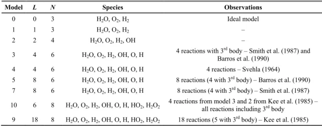
Besides the five physical models, nine different chemical reaction schemes were considered for the frozen and the equilibrium models, taking into account from three to eight species and from null to eighteen chemical reaction equations. The main features of these schemes are summarized at Table 1, where N is the number of chemical species and L is the number of chemical reaction equations. For both frozen and equilibrium flows, different chemical schemes mean at least one different chemical reaction. For non-equilibrium flow, different chemical schemes are related to different efficiencies (of 3rd bodies) and/or different forward reaction rates.

The concept of 3rd _{bodies is associated with the species}

Figure 1. A rocket engine with regenerative cooling.

Table 1. Chemical reaction models for frozen, local equilibrium and non-equilibrium flows.

Model L N Species Observations

0 0 3 H2O, O2, H2 Ideal model

1 1 3 H2O, O2, H2 –

2 2 4 H2O, O2, H2, OH –

3 4 6 H2O, O2, H2, OH, O, H

4 reactions with 3rd body – Smith et al. (1987) and Barros et al. (1990)

4 4 6 H2O, O2, H2, OH, O, H 4 reactions – Svehla (1964)

5 8 6 H2O, O2, H2, OH, O, H 8 reactions (4 with 3rd body) – Barros et al. (1990)

7 8 6 H2O, O2, H2, OH, O, H 8 reactions (4 with 3

rd

body) – Smith et al. (1987)

10 6 8 H2O, O2, H2, OH, O, H, HO2, H2O2

4 reactions from model 3 and 2 from Kee et al. (1985) – all reactions including 3rd body

9 18 8 H2O, O2, H2, OH, O, H, HO2, H2O2 18 reactions (5 with 3rd body) – Kee et al. (1985)

Coolant flow

Once the cross-section area of the rocket engine varies axially, the coolant channels width a (Fig. 1) is not constant, even if the channels height b is. The area variation effect on coolant channels is taken into account, though a one-dimensional model for coolant flow is employed. One-dimension coolant flow comes to the need for quick computational results for thermal analysis of regenerative cooled engines (Naraghi and Foulon, 2008). In this case, only four equations are needed for the quasi-one-dimensional coolant flow: the mass conservation, the momentum conservation, the energy conservation and a polynomial constitutive relation for density. These equations are basically the same ones presented by Rubin and Hinckel (1993) and Marchi et al. (2004). The interaction between the coolant and the combustion gases flows is done by an additional source term in energy equation.

Heat conduction through the wall

As the combustion gases products have high temperature values, heat is transferred from them to thrust chamber walls by convection and radiation mechanisms. This energy is then conducted through walls to the coolant and transmitted to it by convection, respecting the energy conservation principle. Based on this, making a heat balance on the wall surfaces, as presented by Marchi et al. (2004), the temperature of the rocket engine wall is evaluated.

Numerical Model

The mathematical models for reaction gas products and coolant flows (assembly to the heat conduction through the wall) are discretized using the finite volume method (Maliska, 2004; Versteeg

and Malalasekera, 2007). The domain is divided into Nvol control volumes, in both axial directions x and s (Fig. 1). For combustion gases products, a co-located grid arrangement and a methodology appropriated for all the speed flows (Marchi and Maliska, 1994) are used, associated to the second-order central-differencing scheme (CDS), with deferred correction (Lilek et al., 1997). Similar treatment is given to the coolant flow model, except by the fact that the density is provided by a function of the temperature only and not dependent on both the temperature and the static pressure. The systems of algebraic equations obtained are solved by the Tri-Diagonal Matrix Algorithm (TDMA) (Versteeg and Malalasekera, 2007).

Pressure and velocity are coupled by the SIMPLEC algorithm (Van Doormaal and Raithby, 1984), in order to convert the mass equation in a pressure-correction one. Hence, the mass conservation equation is used for the determination of a pressure-correction (P'), while velocity (u) and temperature (T) are obtained from the momentum and the energy equations, respectively. Density (ρ) is obtained from the state equation. The combustion gases composition is evaluated for each control volume, in all the iterations, for local equilibrium and non-equilibrium flows. For this last model, the species-mass conservation equation is also solved.

The boundary conditions for the gases flow at the inlet are: the temperature (T) and the pressure (P) evaluated as functions of the stagnation parameters (T0 and P0); the chemical mixture

composition, obtained from local data (temperature, pressure and the oxidant/fuel ratio, OF); and the entrance velocity (u), estimated by a linear extrapolation from the values obtained in the internal flow. At the exit of the nozzle, temperature (T), velocity (u), pressure (P) and mass fractions (Yi) are obtained by linear extrapolations from internal control volumes.

For the coolant flow, the boundary conditions are: for the channels inlet, both the temperature and the velocity are fixed (Tin

and uin) and the pressure is obtained from linear extrapolation of the internal flow values; the density, for both the inlet and the exit, is estimated by a constitutive relation; the exit pressure is defined as null and both the exit temperature and the exit velocity are obtained by linear extrapolation of internal flow values.

The numerical model implemented consists in simulating the coolant flow in one channel and multiplying the heat transfer values obtained by the number of channels. The coupling between the gases and the coolant flows is made by the heat conduction through the thrust chamber wall, according to the procedures presented by Marchi et al. (2004).

Definition of the Problem

The geometry used in this work is the same one presented by Marchi et al. (2004). It consists of a cylindrical section, called combustion chamber (with radius rin and length Lc) assembled to a nozzle device, whose longitudinal section is defined by a cosine curve (with throat nozzle radius rg and length Ln). The radius r, for

, is evaluated by the following equation: Lc x>

(

)

(

)

⎡ _π −

+ − + = Ln Lc x r r r

r _g in g 1 cos 2

2

(7)

where x corresponds to the axial position where the radius is evaluated. Although the cylindrical section is called combustion chamber, it does not correspond to a real one, once the effects of the fuel, and the oxidant injection, mixture and burning are not considered.

Some parameters of interest taken into account in this work are the nozzle discharge coefficient and the non-dimensional momentum thrust. Both of them are global parameters and evaluate how much the experimental values (laboratorial or numerical ones) are distant from the theoretical values (quasi-one-dimensional isentropic flow). In this work, the experimental values are always related to the numerical ones.

The nozzle discharge coefficient (Cd) and the non-dimensional momentum thrust (F*) are defined as:

th exp m m Cd & &

= (8)

(

)

(

)

exp * ex ex u m u m F & &

= (9)

where m& corresponds to the gases mass flow flux; uex is the exit velocity; and the indexes exp and th refer to experimental and theoretical values, respectively.

In this work, the combustion chamber total length (LT) is equal to 0.5 m, in which 0.1 m is related to combustion chamber length (Lc) and the nozzle length (Ln) is 0.4 m. The nozzle entrance radius (rin) is 0.3 m, while the nozzle throat radius (rg) is 0.1 m. The stagnation properties are T0 = 3420.33 K and P0 = 2.0 MPa, while

the ratio between specific heats is 1.1956, the gas constant (R) is 526.97 J/kg.K, the oxidant/fuel ratio is the stoichiometric one (OF = 7.936682739) and the average wall-gases emissivity is equal to 0.25. Water flows in the regenerative cooling system, through 200 channels, with a total mass flow rate of 200 kg/s and an inlet temperature of 300 K. Although the fin thickness (t = 1.5 mm), the fin height (b = 5.0 mm) and the number of channels are constants, the ratio between the fin height and the channels width (b/a) varies between 0.62 and 2.8, because of the radius nozzle variation along the x-axis.

Discretization Errors

The continuous improvement of the computer resources leads to the opportunity of describing natural phenomena at previously unimaginable scales. This access and this opportunity have served as strong drivers for computational sciences and engineering, especially in the last 20 years (Ghanem, 2009). The consequences of inaccurate CFD results, nevertheless, are at best wasted time, money and effort and at worst catastrophic failure of components, structures or machines. Hence, to address the issue of trust and confidence in CFD, the estimation of numerical errors has a fundamental importance (Versteeg and Malalasekera, 2007).

Numerical errors are composed of four elements: truncation, iteration, round-off and programming errors (Marchi and Silva, 2002). When numerical error consists in the contribution of none but the truncation one, it is also called discretization error (Tannehill et al., 1997), which can be estimated by several techniques, most of them based on the Richardson extrapolation (Richardson, 1910). One of the most commonly used is the Grid Index Convergence (GCI) estimator, proposed by Roache (1997):

1) -( φ φ ) , φ

( 1 1p 2

q Fs p

GCI = − (10)

where Fs is the safety factor (which usually has a value that equals to 3, including in this work); ϕ1 and ϕ2 are, respectively, the numerical

solutions for the fine (h1) and coarse (h2) grids; q is the grid

refinement ratio (q=h₂/h₁); h is the grid spacing or distance

between two successive grid points; and p is related to the asymptotic (pL) or the apparent (pU) order – the lowest value between the two ones (Marchi and Silva, 2002). The asymptotic order depends on the chosen discretization model, while the apparent order, for constant refinement ratio, is evaluated by (Marchi and Silva, 2002):

) log( ) φ φ ( ) φ φ ( log )

( 1 2

3 2 1 q h p_U ⎥ ⎦ ⎤ ⎢ ⎣ ⎡ − −

= (11)

in which ϕ3 corresponds to the numerical solution in a supercoarse

grid (h3) and q=h3 h2=h2 h1.

Numerical Results

Isentropic one-species flow with constant properties

Preliminary studies on the use of GCI estimator for compressible flow are made using the adiabatic isentropic one-species flow with constant properties, which allows the comparison between the numerical uncertainties and the true error. Eleven grids, from 10 up to 10,240 volumes with a refinement ratio of 2, are employed. The asymptotic (a priori) and the apparent (a posteriori) orders (pL and pU, respectively) of the numerical error behaviour in relation to the grid element size (h) are presented in Fig. 2. As can be seen, the apparent order tends to the asymptotic one for all the variables analysed, with the grid refinement, as expected.

10-3 ₁₀-2 ₁₀-1 0.5

1.0 1.5 2.0 2.5 3.0 3.5 4.0

pU

or

pL

h

p_L - all the variables p_U - C_d p_U - F* p_U - P_ex p_U - T_ex p_U - u_ex p_U - M_ex

Figure 2. Asymptotic and apparent orders for all the variables of interest.

Table 2. Numerical solutions for isentropic flow, with error estimates.

Number of volumes Variable of interest Analytical solution

80 1280 10240

Cd [adim.] 1.000000000 1.000 ± 3x10

-3

0.999999 ± 6x10-6 0.99999998 ± 7x10-8

F* [adim.] 1.000000000 1.001 ± 4x10-3 1.000001 ± 5x10-6 1.00000002 ± 6x10-8 Pex [Pa] 29173.41883 2.912x10

4

± 8x101 29173.1 ± 9x10-1 29173.41 ± 1x10-2

Tex [K] 1712.740924 1710 ± 7 1712.73 ± 3x10-2 1712.7408 ± 5x10-4

uex [m/s] 3316.715006 3319 ± 7 3316.72 ± 3x10

-2

3316.7152 ± 4x10-4 Mex [adim.] 3.192834585 3.20 ± 1x10-2 3.19285 ± 5x10-5 3.1928349 ± 8x10-7

Physical and chemical models

Despite the fact that nine chemical schemes are available in the implemented code (for frozen and local equilibrium flows), only results for 6 and 8-species models are presented. This decision is taken based on preliminary studies, in which the other chemical schemes do not present good accuracy compared to CEA (Glenn Research Center, 2005) results. CEA (Chemical Equilibrium with Applications) is a program provided by the Glenn Research Center, a laboratory related to the NASA, which solves frozen and local equilibrium flows for adiabatic one-dimensional conditions. For the non-equilibrium model, results of two chemical models (31 and 32) are presented. The chosen chemical models (3 and 10 for frozen/local equilibrium flows) have good accuracy to the CEA results, with better CPU performance in comparison to their counterparts, although numerical results for chemical models which present the same species are always identical to each other.

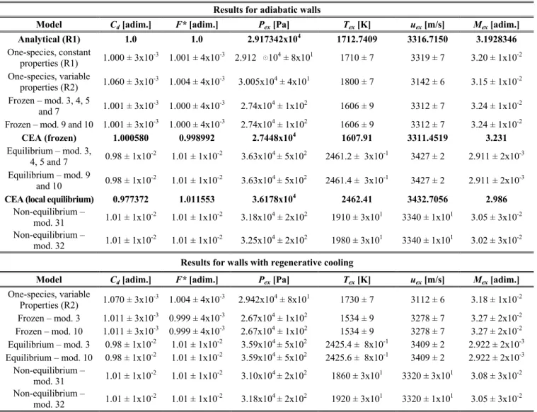
Numerical results for all the variables of interest, including the discretization error estimates, for the 80-volumes grid are presented in Table 3. Six and eight species schemes, for both frozen and equilibrium models and adiabatic or regeneratively cooled walls, present the same results. It means that the inclusion of new species (HO2 and H2O2) has no important role on either the flow conditions

or the variables of interest. Once the increasing of the number of species is related to the growth of the numerical model complexity, six species are preferable to eight species schemes.

Fixing the physical model, based on results in Table 3, it is seen that the heat transfer effects, related to the regenerative cooling system, present only small influence on the global variables of interest (Cd and F*): it is no greater than 1.0%, which is overlapped by the error estimates. The presence of the cooling system, however, is observed for the local variables of interest (Pex, Tex, uex and Mex),

for which the variation is about 1.0 to 4.5% (out of the uncertainties range), depending on the physical model and on the variable of interest considered. Such difference is caused by the fact that the global variables of interest are related to the mass flux flow and the local variables are strongly related to the energy of the flow. While the mass flow through the nozzle, with or without regenerative cooling, is basically the same, the presence of the cooling system reduces the energy of the gases flow by the heat transfer to the coolant. In this way, the presence of the cooling system has smaller effects on Cd and F* and stronger effects on Pex, Tex, uex and Mex.

Cooling system

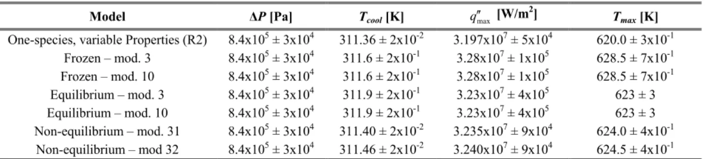
Table 4 provides the numerical results for the coolant properties as well as for the heat transfer parameters: the coolant pressure drop through the channels (∆P), the exit coolant temperature (Tcool), the

maximum heat flux to the coolant ( ) and the maximum wall

temperature (T

max

q′′

max). As can be seen, numerical results are quite independent of the physical model choice: in all the physical models studied, the coolant pressure drop is exactly the same. For the exit coolant temperature, only a small variation is observed (0.54 K, at maximum); it is, however, a bit larger than the numerical uncertainty (0.2 K), and can be attributed to the differences among the physical models. Larger differences are observed for the maximum heat flux: it achieves 8.3x105 W/m2 (comparing the one-species gas to the frozen flow models), what can also be related to the physical models. The effect of such variation on the maximum wall temperature, however, is quite small: only 8.5 K (for the same physical models) and, if frozen and equilibrium results are compared, this difference is even smaller: 5.5 K. Such variation, however, is larger than the numerical uncertainty ranges and can again be attributed to the physical model differences.

Table 3. Numerical results and error estimates for the 80-volumes grid.

Results for adiabatic walls

Model Cd [adim.] F* [adim.] Pex [Pa] Tex [K] uex [m/s] Mex [adim.]

Analytical (R1) 1.0 1.0 2.917342x104 1712.7409 3316.7150 3.1928346

One-species, constant

properties (R1) 1.000 ± 3x10

-3

1.001 ± 4x10-3 2.912 ּ◌104 ± 8x101 1710 ± 7 3319 ± 7 3.20 ± 1x10-2

One-species, variable

properties (R2) 1.060 ± 3x10

-3

1.004 ± 4x10-3 3.005x104 ± 4x101 1800 ± 7 3142 ± 6 3.15 ± 1x10-2

Frozen – mod. 3, 4, 5

and 7 1.001 ± 3x10

-3

1.000 ± 4x10-3 2.74x104 ± 1x102 1606 ± 9 3312 ± 7 3.24 ± 1x10-2

Frozen – mod. 9 and 10 1.001 ± 3x10-3 1.000 ± 4x10-3 2.74x104 ± 1x102 1606 ± 9 3312 ± 7 3.24 ± 1x10-2

CEA (frozen) 1.000580 0.998992 2.7448x104 1607.91 3311.4519 3.231

Equilibrium – mod. 3,

4, 5 and 7 0.98 ± 1x10

-2

1.01 ± 1x10-2 3.63x104 ± 5x102 2461.2 ± 3x10-1 3427 ± 2 2.911 ± 2x10-3

Equilibrium – mod. 9

and 10 0.98 ± 1x10

-2

1.01 ± 1x10-2 3.63x104 ± 5x102 2461.4 ± 3x10-1 3427 ± 2 2.911 ± 2x10-3

CEA (local equilibrium) 0.977372 1.011553 3.6178x104 2462.41 3432.7056 2.986

Non-equilibrium –

mod. 31 1.01 ± 1x10

-2

1.01 ± 1x10-2 3.18x104 ± 2x102 1910 ± 3x101 3340 ± 1x101 3.05 ± 3x10-2

Non-equilibrium –

mod. 32 1.01 ± 1x10

-2

1.01 ± 1x10-2 3.25x104 ± 2x102 1980 ± 3x101 3340 ± 1x101 3.02 ± 3x10-2

Results for walls with regenerative cooling

Model Cd [adim.] F* [adim.] Pex [Pa] Tex [K] uex [m/s] Mex [adim.] One-species, variable

Properties (R2) 1.070 ± 3x10

-3

1.004 ± 4x10-3 2.942x104 ± 8x101 1730 ± 7 3112 ± 6 3.18 ± 1x10-2

Frozen – mod. 3 1.011 ± 3x10-3 0.999 ± 4x10-3 2.67x104 ± 1x102 1534 ± 9 3278 ± 7 3.27 ± 2x10-2

Frozen – mod. 10 1.011 ± 3x10-3 0.999 ± 4x10-3 2.67x104 ± 1x102 1534 ± 9 3278 ± 7 3.27 ± 2x10-2

Equilibrium – mod. 3 0.98 ± 1x10-2 1.01 ± 1x10-2 3.59x104 ± 5x102 2425.4 ± 8x10-1 3409 ± 2 2.922 ± 2x10-3 Equilibrium – mod. 10 0.98 ± 1x10-2 1.01 ± 1x10-2 3.59x104 ± 5x102 2425.6 ± 8x10-1 3409 ± 2 2.922 ± 2x10-3

Non-equilibrium –

mod. 31 1.01 ± 1x10

-2

1.01 ± 1x10-2 3.10x104 ± 2x102 1860 ± 3x101 3320 ± 3x101 3.08 ± 3x10-2

Non-equilibrium –

mod. 32 1.01 ± 1x10

-2

1.01 ± 1x10-2 3.18x104 ± 2x102 1920 ± 3x101 3320 ± 1x101 3.05 ± 3x10-2

(R1): Rg = 526.97 J/kgK; (R2): Rg = 461.525 J/kgK (equivalent to combustion gases mixture for the ideal model)

Figures 3 and 4 provide the temperature distribution for both the gases flow and the wall, respectively, for different physical models. While the physical models have an important role on the temperature of the gases flow, as can be seen in Fig. 3, the distribution of the wall temperatures are little affected by them, Fig. 4, especially at the nozzle throat, where the critical temperature of the whole structure is achieved. In Fig. 3, it is also included numerical results of CEA for both adiabatic frozen and local equilibrium flows, with good concordance between CEA and the ones obtained by the implemented code. In that figure, it is also clear the secondary role of the cooling system on the distribution of the gases flow, once it is only small affected through the whole nozzle profile. It can also be noticed that there is no simple correlation between the highest temperature of the gases flow and the highest temperature at the wall: while temperatures associated to the local equilibrium flow are always higher than the other physical models, as seen in Fig. 3, the highest wall temperature is achieved when the frozen flow model is employed (Fig. 4), which corresponds to the lowest temperature profile through the nozzle.

The higher values for the wall temperatures in the frozen flow model from the thrust chamber entrance to the throat region, seen at Fig. 4, can be explained by differences observed in the convection coefficient: while it achieves 11,691 W/m2K in the nozzle throat

region for the frozen flow, it is about 10,861 W/m2K for the local equilibrium. Thus, even though the local equilibrium model presents recombination reactions, which are exothermic and contribute to higher gases temperatures, the more elevated values for convection coefficient verified for the frozen flow overtake these effects. Because of this, the highest wall temperatures are associated to the frozen model, in spite of the local equilibrium one. Otherwise, the difference between frozen flow and equilibrium flow reaction gas temperatures after the nozzle throat region becomes so expressive that the effects of the more elevated values for convection coefficient are overtaken by the higher gases temperatures of the local equilibrium flow. Because of this, the wall temperatures, from the nozzle throat to the thrust chamber exit, are higher for the local equilibrium model.

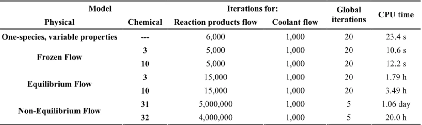
CPU time

flows, as the number of global iterations employed. The number of iterations was high enough to guarantee the achievement of the round-off error for each sub-problem separately, in each global iteration. The only exception was the non-equilibrium flow, for which a tolerance (for the ratio between both the heat transfer rate from the reactive gases flow and the heat transfer rate received by the coolant) of 10-5 was specified by CPU time restrictions. The adopted procedure was needed to minimize the other components of the numerical error to none, but the truncation one (in this case, also named discretization error), in order to allow the use of the GCI estimator.

According to Tab. 5, six species models needed about 87% of the CPU time required by the eight species ones for the frozen flow,

and about 51% of the CPU time of the eight-species for the local equilibrium one. Once the numerical results are the same for both chemical species schemes, six species models should be preferred by the lowest CPU time. Considering the coolant properties and the wall temperatures, seen at Tab. 4, and the CPU time, at Tab. 5, the preferable physical model might be the frozen one. This choice is based on the fact that such model provides the upper bound values for both the temperature and the heat flux in the wall, which are the most critical features in the rocket engine design, with the lowest CPU time: studies with the frozen flow model are at least 500 times faster than the ones with the local equilibrium model and 5,500 times faster the than non-equilibrium ones.

Table 4. Numerical results for the coolant flow and the wall temperature for the 80-volumes grid.

Model ΔP [Pa] Tcool [K] qmax′′ [W/m

2

] Tmax [K] One-species, variable Properties (R2) 8.4x105 ± 3x104 311.36 ± 2x10-2 3.197x107 ± 5x104 620.0 ± 3x10-1

Frozen – mod. 3 8.4x105 ± 3x104 311.6 ± 2x10-1 3.28x107 ± 1x105 628.5 ± 7x10-1

Frozen – mod. 10 8.4x105 ± 3x104 311.6 ± 2x10-1 3.28x107 ± 1x105 628.5 ± 7x10-1

Equilibrium – mod. 3 8.4x105 ± 3x104 311.9 ± 2x10-1 3.23x107 ± 4x105 623 ± 3

Equilibrium – mod. 10 8.4x105 ± 3x104 311.9 ± 2x10-1 3.23x107 ± 4x105 623 ± 3

Non-equilibrium – mod. 31 8.4x105 ± 3x104 311.40 ± 2x10-2 3.235x107 ± 9x104 624.0 ± 4x10-1

Non-equilibrium – mod 32 8.4x105 ± 3x104 311.46 ± 2x10-2 3.240x107 ± 9x104 624.5 ± 4x10-1

(R2): Rg = 461.525 J/kgK (equivalent to combustion gases mixture for the ideal model)

0.0 0.1 0.2 0.3 0.4 0.5

1600 1800 2000 2200 2400 2600 2800 3000 3200 3400 3600

Without regenerative cooling Isentropic (analytical solution) CEA (frozen)

Mod. 3 (frozen) CEA (eq.) Mod. 3 (eq.) Mod. 31 (non-eq.) Mod. 32 (non-eq.) Nozzle profile

With regenerative cooling Mod. 3 (frozen) Mod. 3 (eq.) Mod. 31 (non-eq.) Mod. 32 (non-eq.)

x [m]

T

em

p

er

atu

re [

K

]

Figure 3. Temperature of the gases through the nozzle.

0.0 0.1 0.2 0.3 0.4 0.5

425 450 475 500 525 550 575 600 625

one-species, var. prop. frozen, mod. 3 equilibrium, mod. 3 non-eq., mod. 31 non-eq., mod. 32 nozzle profile

x [m]

Tem

p

era

ture [K]

Figure 4. Temperature of the nozzle wall in contact with the gases.

Table 5. CPU time for the regeneratively cooled nozzle (80-volumes grid).

Model Iterations for:

Physical Chemical Reaction products flow Coolant flow

Global

iterations CPU time

One-species, variable properties --- 6,000 1,000 20 23.4 s

3 5,000 1,000 20 10.6 s

Frozen Flow

10 5,000 1,000 20 12.2 s

3 15,000 1,000 20 1.79 h

Equilibrium Flow

10 15,000 1,000 20 3.49 h

31 5,000,000 1,000 5 1.06 day

Non-Equilibrium Flow

32 4,000,000 1,000 5 20.0 h

Conclusion

Numerical studies for a regeneratively cooled rocket engine were performed, taking into account different physical and chemical models. For all the results, numerical uncertainties were evaluated by the GCI estimator and comparisons between the numerical results provided by the implemented code and the NASA's code CEA provided good concordance, for adiabatic nozzle conditions.

The main results of this work can be summarized as follows:

1. GCI estimator can be employed for compressible flows,

providing accurate results for the numerical uncertainties. 2. Numerical results for the 80-volumes grid are as accurate as the

experimental ones, with numerical and experimental uncertainties of the same magnitude.

3. There are not significant differences on the numerical results between six and eight species models for both frozen and local equilibrium flows. The major difference is observed in the CPU time requirements, which is higher for the eight species models. 4. The assembling of the refrigeration effects to the gases flow has

only small influence on the global parameters of interest in the nozzle. For local parameters of interest, otherwise, larger differences were observed, which can be related to the differences among the physical models.

5. The choice of the physical model has little influence in the coolant parameters, such as the pressure drop and the coolant exit temperature. For the maximum heat flux and the maximum wall temperature, however, the differences are more expressive. 6. Once the frozen flow model presents the upper bound values for

both the maximum heat flux and the maximum temperature in the wall (two of the most important features in the rocket engine design), with lower CPU time, this model should be the preferable one, at least for preliminary studies.

Acknowledgements

The authors would like to acknowledge the Department of Mechanical Engineering (DEMEC), the Federal University of Parana (UFPR), CAPES – Coordenação de Aperfeiçoamento de Pessoal de Nível Superior, CNPq – Conselho Nacional de Desenvolvimento Científico e Tecnológico and the UNIESPAÇO Program of the Brazilian Space Agency (AEB) for physical and financial support given to this work. The second author is supported by a scholarship from CNPq. The authors thank the Associate Editor for his suggestions and comments.

References

AIAA, 1998, “Guide for the Verification and Validation of Computational Fluid Dynamics Simulations”, AIAA G-077-1998.

Anderson Jr., J.D., 2003, “Modern Compressible Flow with Historical Perspective”, 3 ed., McGraw-Hill, New York, United States, 760 p.

Barros, J.E.M., Alvin Filho, G.F. and Paglione, P., 1990, “Estudo de Escoamento Reativo em Desequilíbrio Químico através de Bocais Convergente-Divergente” (in Portuguese), Proceedings of the 3rd Brazilian Congress of Thermal Engineering and Sciences, Itapema, Brazil, pp. 771-776.

Dunn, S.S. and Coats, D.E., 1997, “Nozzle Performance Predictions Using the TDK 97 Code”, AIAA 97-2807, Proceedings of the 33rd Joint Propulsion Conference and Exhibit, Seattle, United States, pp. 1-13.

Glenn Research Center, 2005, CEA – Chemical Equilibrium with Applications, available at: <http://www.grc.nasa.gov/WWW/CEAWeb/ceaHome.htm>, access in: Feb 16, 2005.

Ghanem, R.G., 2009, “Uncertainty Quantification in Computational and

Prediction Science”, International Journal for Numerical Methods in

Engineering, Vol. 80, pp. 671-672.

Habiballah, M., Vingert, L., Duthoit, V. and Vuillermoz, P., 1998, “Research as a Key in the Design Methodology of Liquid-Propellant

Combustion Devices”, Journal of Propulsion and Power, Vol. 14, pp. 782-788.

Kee, R.J., Grcar, J.F., Smooke, M.D., and Miller, J.A., 1985, “A Fortran Program for Modeling Steady Laminar One-Dimensional Premixed Flames”, Sandia National Laboratories, SAND85-8240.

Kuo, K.K., 2005, “Principles of Combustion”, 2 ed., John Wiley & Sons, New York, United States, 732 p.

Lilek, Z., Muzaferija, S. and Perić, M., 1997, "Efficiency and Accuracy

Aspects of a Full-Multigrid Simple Algorithm for Three-Dimensional

Flows", Numerical Heat Transfer, Part B, Vol. 31, pp. 23-42.

Maliska, C.R., 2004, “Transferência de Calor e Mecânica dos Fluidos Computacional”, LTC Editora, Brazil, 453 p.

Marchi, C.H. and Maliska, C.R., 1994, “A Nonorthogonal Finite Volume Method for the Solution of all Speed Flows Using Co-Located

Variables”, Numerical Heat Transfer, Part B, Vol. 26, pp. 293-311.

Marchi, C.H. and Silva, A.F.C., 2002, “Unidimensional Numerical

Solution Error Estimation for Convergent Apparent Order”, Numerical Heat

Transfer, Part B, Vol. 42, pp. 167-188.

Marchi, C.H., Laroca, F., Silva, A.F.C. and Hinckel, J.N., 2004, “Numerical Solutions of Flows in Rocket Engines with Regenerative

Cooling”, Numerical Heat Transfer, Part A, Vol. 45, pp. 699-717.

Naraghi, M.H., and Foulon, M., 2008, “A Simple Approach for Thermal Analysis of Regenerative Cooling of Rocket Engines”, Proceedings of the 2008 ASME International Mechanical Engineering Congress and Exhibition, Boston, United States, pp. 1-8.

Metha, U.B., 1996, “Guide to Credible Computer Simulations of Fluid

Flows”, Journal of Propulsion and Power, Vol. 12, pp. 940-948.

Oberkampf, W.L., and Trucano, T.G., 2008, “Verification and Validation

Benchmarks”, Nuclear Engineering and Design, Vol. 238, pp. 716-743.

Richardson, L.F., 1910, “The Approximate Numerical Solution by Finite Differences of Physical Problems involving Differential Equations, with an

Application to the Stresses in a Masonry Dam”, Philosophical Transactions

of the Royal Society of London, Series A, Vol. 210, pp. 307-357.

Roache, P.J., 1994, “Perspective: A Method for Uniform Reporting of Grid

Refinement Studies”, Journal of Fluids Engineering, Vol. 116, pp. 405-413.

Roache, P.J., 1997, “Quantification of Uncertainty in Computational

Fluid Dynamics”, Annual Review of Fluid Mechanics, Vol.29, pp. 129-160.

Rubin, R.L. and Hinckel, J.N., 1993, “Regenerative Cooling for Liquid Propellant Rocket Thrust Chambers”, Proceedings of the 12th Brazilian Congress of Mechanical Engineering, Brasília, Brazil, pp. 737-740.

Smith, T.A., Pavli, A.J. and Kacynski, K.J., 1987, “Comparison of Theoretical and Experimental Thrust Performance of a 1030:1 Area Ratio Rocket Nozzle at a Chamber Pressure of 2413 kN/m2 (350 psia)”, NASA Lewis Research Center, NASA Technical Paper 2725.

Sutton, G.P. and Biblarz, O., 2001, “Rocket Propulsion Elements”, 7 ed., John Wiley & Sons, New York, United States, 751 p.

Svehla, R.A., 1964, “Thermodynamic and Transport Properties for the Hydrogen-Oxygen System”, NASA Lewis Research Center, NASA SP-3011.

Szabó B. and Babuska, I., 1991, “Finite Element Analysis”, Wiley & Sons., New York, United States, 380 p.

Tannehill, J.C., Anderson, D.A. and Pletcher, R.H., 1997, “Computational Fluid Mechanics and Heat Transfer”, 2 ed., Taylor & Francis, Philadelphia, United States, 790 p.

Van Doormaal, J.P. and Raithby, G.D., 1984, “Enhancements of the

SIMPLE Method for Predicting Incompressible Fluid Flow”, Numerical

Heat Transfer, Vol. 7, pp. 147-163.

Versteeg, H.K., Malalasekera, W., 2007, “An Introduction to Computational Fluid Dynamics: The Finite Volume Method”, 2 ed., Pearson Education Limited, Harlow, England, 503 p.

Wang, T.S., 2006, “Multidimensional Unstructured-Grid Liquid

Rocket-Engine Nozzle Performance and Heat Transfer Analysis”, Journal of

Propulsion and Power, Vol. 22, pp. 78-84.

Wang, T.S., 2009, “Transient Three-Dimensional Startup Side Load Analysis

of a Regeneratively Cooled Nozzle”, Shock Waves, Vol. 19, pp. 251-264.

Wang, T.S., and Guidos, M., 2009, “Transient Three-Dimensional Side

Load Analysis of a Film-Cooled Nozzle”, Journal of Propulsion and Power,

Vol. 25, pp. 1272-1280.

Zhang, H.W., He, Y.L., and Tao, W.Q., 2007, “Numerical Study of Film

and Regenerative Cooling in a Thrust Chamber at High Pressure”, Numerical

Heat Transfer, Part A, Vol. 52, pp. 991-1007.

Zhang, X.D., Pelletier, D., Trépanier, J.-Y. and Camarero, R., 2001,

“Numerical Assessment of Error Estimators for Euler Equations”, AIAA

Journal, Vol. 39, pp. 1706-1715.