Hélio Aparecido Navarro
[email protected] Universidade de São Paulo – USP Escola de Engenharia de São Carlos Departamento de Engenharia Mecânica 13566-590 São Carlos, SP, BrazilLuben Cabezas-Gómez
[email protected] Pontifícia Universidade Católica de Minas Gerais Departamento de Engenharia Mecânica 30535-901 Belo Horizonte, MG, BrazilJoão R. Bastos Zoghbi Filho
[email protected]Gherhardt Ribatski
[email protected] Universidade de São Paulo – USP Escola de Engenharia de São Carlos Departamento de Engenharia Mecânica 13566-590 São Carlos, SP, BrazilJosé Maria Saiz-Jabardo
[email protected] Universidad de la Coruña Escuela Politécnica Superior 15403 Ferrol, Coruña, SpainEffectiveness - NTU Data and
Analysis for Air Conditioning and
Refrigeration Air Coils
A simulation program based on a control volume analysis has been used in the evaluation of the (ε, NTU) relationship for coils of complex geometry and flow arrangement. The simulation program has been evaluated through simple geometry and flow arrangement coils. The program results compare very well with correlations for simple cross flow coils, and a number of rows up to four. It has also been determined that closed form correlations developed for coils of an infinite number of tube rows are inadequate for those with number of rows in the range between 5 and 10. In addition, it has been found that closed form (ε, NTU) correlations for cross flow coils with the same tube arrangement and number of rows might lead to inaccuracies higher than 10% in the evaluation of the effectiveness of coils of complex flow arrangement.
Keywords: effectiveness, NTU, air coil
Introduction
1
Refrigeration and air conditioning air coils present a wide range of geometric configurations and flow arrangements. They are part of the family of the so-called “compact heat exchangers”, Kays and London (1998). Overall analysis of this kind of heat exchanger has been generally made through the so-called (ε, NTU) procedure, as suggested by Kays and London (1998). One of the problems faced by the designer in using this procedure is to find adequate correlations between the coil effectiveness, ε, and the Number of Transfer Units, NTU. These correlations involve other coil parameters such as the ratio between fluids heat capacity rates, the geometry, and the relative flow arrangement of the fluids. During the past fifty years, several studies have been dedicated to the development of (ε, NTU) correlations for compact heat exchangers. One of the best-known publications is the book by Kays and London (1998), referred above, which contains graphical and table information relating to the effectiveness and the Number of Transfer Units for numerous compact heat exchangers for different geometries and flow arrangements. Despite its completeness, the Kays and London text does not cover some of the coil arrangements used in the refrigeration and air conditioning industry. Bowman et al. (1940) addressed the problem by calculating the factor F, for the mean logarithmic temperature difference, for cross flow, several pass heat exchangers. Later on, Stevens et al. (1957) proposed closed form series correlations and plots for cross flow, multiple
Paper accepted January, 2010. Technical Editor: José A. dos Reis Parise
row heat exchangers, including the three possible arrangements of the fluids: unmixed/unmixed, mixed/unmixed, and both mixed. Pignotti and Cordero (1983) proposed closed form expressions for the factor F of the logarithmic mean temperature for several arrangements of cross flow compact heat exchangers. Later on Pignotti (1988) suggested a matrix formalism for the evaluation of the thermal effectiveness of complex heat exchangers configurations that can be broken into simple constitutive parts, connected to each other by unmixed streams. Baclic (1990) provided a list of closed form (ε, NTU) correlations for a number of flow arrangements used in compact heat exchangers. Pignotti and Shah (1992) discussed some methods for the determination of the (ε, NTU) relationship for complex heat exchanger flow arrangements, among them the Domingos’ rules (1969), the chain rule and the rules for heat exchangers with a mixed fluid. Eighteen (ε, NTU) closed form correlations were developed from these rules. Pignotti and Shah (1993) considered complex heat exchanger flow arrangements and related them to simple ones for which a closed form either is available or an approximate solution can be obtained. Wang et al. (2000) referred to several (ε, NTU) correlations developed by the 1998 ESDU (Engineering Science Data Unit) version for coils of complex geometry, including those with parallel circuits of the tube fluid and several rows, typical of those used in the refrigeration and air conditioning industry.
but used local heat transfer coefficients instead of average ones extensive to the overall heat exchanger area. Vardham and Dhar (1997) proposed a model that, similarly to the previous ones, divides the coil into finite volumes along the tube fluid path and carries out iterative marches between the tube fluid entrance and exit, while simultaneously updating the air-side properties. In each volume element, the effectiveness is computed as if it were a mixed/unmixed cross flow heat exchanger. Corberán and Melón (1998) used similar approach as the others to simulate evaporation and condensation of refrigerant R-134a in order to check the performance of different change of phase correlations.
In the present study, a computer simulation program has been used to raise effectiveness – NTU data for coils of complex geometry and flow arrangements. The present paper uses the same approach of works published by Navarro and Cabezas-Gómez (2005) and Cabezas-Gómez et al. (2007). To follow a description of the working model and computer simulation program is provided for reader information. Then, the program performance is evaluated for coils of simpler geometry for which closed form (ε, NTU) relations are available. Finally, this program is used in developing (ε, NTU) plots for air conditioning and refrigeration air coils with complex flow arrangement.
Nomenclature
A = overall heat transfer area of the coil, m2 C = heat capacity rate, W/K
C* = heat capacity ratio, Cmin/Cmax, dimensionless L = length of the tube, m
m& = mass flow rate, Kg/s Nc = number of tube fluid circuits Ne = number of elements per tube Nr = number of rows
Nt = number of tubes per row
NTU = number of transfer units, (UA/Cmín) q = heat transfer rate, kW
Pl = longitudinal pitch of tubes, m Pt = transversal pitch of tubes, m T = temperature, °C
U = overall heat transfer coefficient, W/(m2 K)
Greek Symbols
Δ = denotes difference
ε = effectiveness of heat exchanger Γ = effectiveness of the tube element δ = deviation
Subscripts
a air side av average i inlet max higher value min lower value o outlet t tube side
Superscripts
e element
Governing Equations for Tube Elements
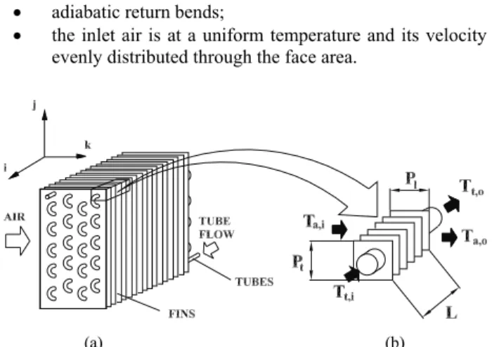
The geometry of the air coil considered in the present study is schematically shown in Fig. 1(a). The fluid flowing inside the tubes is designated as “tube fluid”. Air flows externally to the tubes, in the space between fins, in a general cross flow configuration. The model consists in dividing the air coil in small (finite) volumes
designated as “tube elements”, each encompassing a segment of tube and the corresponding fins, as illustrated in Figs. 1(a) and (b).
The center of a tube element is a nodal point, its spatial location being characterized by the triplet (i, j, k), corresponding to the space directions, as shown in Fig. 1(a). The number of tube elements in each direction is respectively equal to Ne, Nt and Nr, with the first being the number of elements in a tube, the second the number of tubes in a row (tubes in the normal direction to the air flow), and the third the number of rows in the air coil. The tube fluid is distributed into Nc parallel circuits. Finally, the following additional assumptions are considered in model development:
• constant overall heat transfer coefficient and thermodynamic and transport properties;
• adiabatic return bends;
• the inlet air is at a uniform temperature and its velocity is evenly distributed through the face area.
(a) (b)
Figure 1. (a) Schematic representation of the air coil considered in the present study; (b) a tube element.
Energy balances for the tube fluid and air in a tube element can be written as
(
e)
i, t e o , t e t
e C T T
q =− − (1a)
(
e)
i, a e o , a e a e
T T C
q = − (1b)
The superscript “e” refers to the tube element (i, j, k). The product of the element mass flow rate of each fluid by its specific heat have been designated by and , respectively for the tube
fluid and for the air, and will be referred to as “heat capacity rates” for simplification purposes. The mass flow rate of each fluid in the element can be determined from the corresponding overall mass flow rate according to the following equations:
e t
C
C
aet e
a e a
N N
m
m& = & (2a)
c t e t
N m
m& = & (2b)
Since the tube elements are relatively short (the shorter the better), the tube fluid temperature variation is small. Thus, as a first approximation, the tube fluid temperature could be assumed constant in the element. This temperature is assigned to the corresponding nodal point, and can be determined as
(
e)
o , t e i , t e
t . T T
T =05 + (3)
remaining constant. In such a case, the individual thermal effectiveness of each tube element can be written as
⎥⎦ ⎤ ⎢⎣ ⎡ − − = − − = e a C e ) UA ( e ) NTU (
e 1 e 1 e
Γ (4)
Actually, the air heat capacity rate, , is clearly smaller than
the tube fluid one, since the air flow rate is of the same order as the length of the tube element. The product of the overall heat transfer coefficient by the heat transfer area of the element, (UA)
e a
C
e , is given by
( )
r t e e N N N UAUA = (5)
It must be noted that the overall heat transfer coefficient, U, is assumed constant over the air coil. Thus, the remaining terms of the right hand side of Eq. (5) correspond to the heat transfer area of each tube element.
Finally, introducing the definition of heat exchanger effectiveness, a relationship between the temperatures of the fluids and the element effectiveness, , can be established according to the following equation:
e
Γ
(
)
) T T ( T T q q e i , a e i , t e i , a e o , a e máx e − − = ⎟⎟ ⎠ ⎞ ⎜⎜ ⎝ ⎛ =Γ (6)
The exit temperatures of both fluids in each tube element can be obtained through the solution of the above set of equations, providing that the following overall parameters are known: the geometry and the overall heat transfer coefficient, mass flow rate of both fluids, the number of tubes in a row, the number of rows and the number of parallel circuits of the tube fluid along with the number of tube elements for each tube (arbitrarily chosen) and the inlet temperature of both fluids in the element.
Computational Procedure
The air coil simulation program has been developed from the set of governing equations for each tube element described in the preceding section. When the objective is the air coil simulation, the input parameters are the following: geometry, mass flow rates and inlet temperatures of both fluids, and the overall heat transfer coefficient. The exit temperatures of both fluids along with the coil effectiveness would result from this mode of application. In the present paper, the objective is to determine the (ε, NTU) relationship. In this case, using the mass flow rate as an input parameter would not be adequate. As a result, the overall air-coil NTU and the heat capacity rates substitute for the mass flow rates of both fluids as input parameters. Individual tube element heat capacities can thus be determined from the following equations:
• If Cmin = Ca
t e e a N N NTU / UA
C = and
c * e t N C NTU / UA
C = (7a)
• If Cmin = Ct
t e * e a N N C NTU / UA
C = and
c e t N NTU / UA
C = (7b)
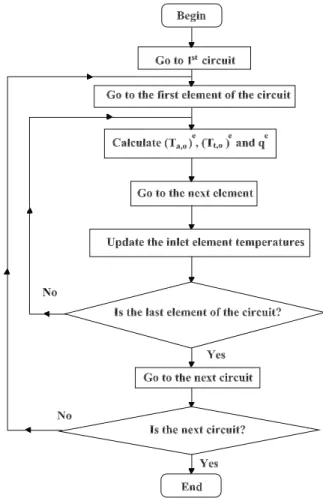
A block diagram of the algorithm for the effectiveness determination (evaluation) is presented in Figs. 2 and 3. A step-by-step discussion will be presented next in order to make it easier to the reader to follow the adopted procedure.
Step 1
Read the input data. The air coil geometry is read from a file containing information such as the number of rows, tubes, and the number of circuits of the tube fluid and their arrangement. The given value of NTU is introduced along with the capacity ratio, C*, and the value of Cmin. The tube element size (length) is also evaluated at this stage. Its value is determined from a trial and error procedure consisting in running the program for an increasing number of tube elements and checking the obtained results. The adequate number of tube elements would be the one that causes no further variation in the determined parameters. An adequate number of elements has been found to be as low as 10. The number of elements actually used throughout the present investigation exceeded the amount considered adequate by a factor of three or more, since in most of the runs, the number of elements was of the order of 100.
Step 2
Arbitrary values are assigned to the overall air coil entrance temperatures of both fluids, Ta,i and Tt,i, and to the product of the overall heat transfer coefficient by the heat transfer area, UA.
Step 3
Values of (UA)e, , and Γe for the tube element are evaluated.
e a
C Cte
Step 4
At this point, the temperature distribution along the air coil is evaluated through the subroutine TEMPERATURE, described in the block diagram of Fig. 3. Starting from the entrance of the tube fluid in one of the parallel circuits, the procedure in this subroutine consists in determining the outlet temperatures of both fluids in successive tube elements in the path of the tube fluid. The starting temperatures are always the air coil inlet temperatures. It must be noted that, depending on the flow arrangement, the actual starting tube element could correspond to one in which the inlet air temperature might not be the air coil inlet temperature. Thus, as a general procedure, the inlet air temperature of the first tube element is assumed to be the one at the air coil entrance, and a trial procedure must be carried out in order to determine the exit air and tube fluid temperatures, as described in the block diagram of Fig. 2. The air and tube fluid temperatures in the tube elements along the particular circuit are determined in the subroutine TEMPERATURE along with the rate of heat transfer in each tube element. In the present step, the first trial is performed.
Step 5
The first trial exit average air temperature is determined, according to the following equation:
e t j , i r e o , a o , a N N ) N , j , i ( T T ∑
Figure 2. Block diagram of the main program.
Step 6
The second trial is performed calling the subroutine TEMPERATURE, using as input data in the tube elements the inlet air temperatures obtained in the first trial. The new exit average air temperature is determined and compared with the old one (previous step). New trials will be performed until the relative difference between the average exit air temperature in successive trials is lower than a given value, δp. The program proceeds to determine overall air coil parameters such as average exit tube fluid temperature, effectiveness, and overall rate of heat transfer, according to the following equations:
c c N
m t,o,m o
,
t N
T T
∑
= =1 (9)
) T T ( C ) T T ( C q
q t t,o ti, a a,o a,i k
, j , i
k , j , i
e =− − = −
∑
= (10)
i , a i , t
max
max T T
T
q q
− =
= Δ
ε (11)
The values of the different terms in Eq. (10), determined independently, must be close enough to each other to warrant the energy conservation.
Figure 3. Block diagram of the subroutine TEMPERATURE.
Program Performance Evaluation
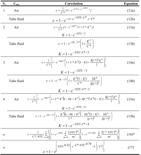
A series of multi-row air coils with in-line tube distribution has been considered for evaluation of the performance of the proposed model. The arrangement is the typical cross-flow, as shown in Fig. 4, where one can also note that the tube fluid is distributed in as many circuits as the number of tube rows. Both fluids flow in an unmixed/unmixed arrangement, except in the coil of Fig. 4(a), for a single tube-fluid circuit. Closed form (ε, NUT) equations are available in the literature for this kind of coils. Some of the ones listed in Table 1 have been proposed by ESDU 98005 (1998) and are valid for different number of tube rows. These correlations also depend on the thermal capacity ratio, C*, and on which of the fluids is the one with lower thermal capacity (either the air or the tube fluid).
adequacy of the simplified form, Eq. (17), for coils with a large
number of rows. ∑
− = N t t s av N 1 100 ε ε ε
δ (19)
The program has been run for values of the heat capacity ratio, C*, varying in the range between 0.1 and 1, and NTU from 0.1 up to a maximum of 6, with increments of 0.1 for each parameter, performing a total of 600 computer program runs. Tables 2 and 3 present a summary of the performed comparisons. Results for coils up to 4 rows are presented in Table 2. Columns 2 and 3, for the two possible conditions of minimum heat capacity rate, present information regarding the maximum absolute relative deviation and the heat capacity ratio and the NTU for which this deviation has been obtained. The resulting deviations can be considered as negligibly small for all practical purposes.
Figure 4. Cross-flow coils geometry for simulation program evaluation.
Two different parameters have been used in the simulation program evaluation: the absolute relative deviation, δ, and the average absolute relative deviation, δav, both of them related to the deviation of simulation program with respect to correlation results. Their expressions are as follows:
t t s ε ε ε
δ=100 − (18)
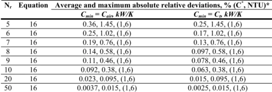
Table 3 presents comparisons of results from the simulation program with those from Eq. (16), used as reference for that purpose. The average absolute relative deviation, extensive to all the data points, has been included in this table in addition to the parameters of Table 2. It can be noted that deviations diminish with the number of rows, as should be expected. Though relatively small, deviations for coils with a number of rows lower than 10 are much higher than those obtained for the other coils. In fact, for the 5 rows coil, the maximum obtained deviation is of the order of 1.45%, threefold that for the 9 rows coil. Results from the simulation program and those from the Stevens et al. (1957) correlation compare very well for coils with more than 20 rows, since, in such cases, the average deviations are lower than 0.023%.
Table 1. Closed form (ε, NTU) correlations for coils with different number of rows according to ESDU (1998).
Nr Cmin Correlation Equation
1 Air [ e ]
* C ) NTU e ( * C −− −
−
= 1 1 1
ε (12a)
Tube fluid ε=1−e−(1−e−NTU⋅C*)/C* (12b)
2 Air [ e ( C*K )]
* C * KC 2 2 1 1 1 + − = − ε (13a) 2
1 e NTU/
K= − −
Tube fluid ⎟⎟
⎠ ⎞ ⎜ ⎜ ⎝ ⎛ + − = − * C K e K/C*
2
2 1
1
ε (13b)
2 1 e NTUC*/
K= − − ⋅
3 Air ( ) ( )
⎥ ⎥ ⎦ ⎤ ⎢ ⎢ ⎣ ⎡ ⎟ ⎟ ⎠ ⎞ ⎜ ⎜ ⎝ ⎛ + − + − = − 2 3 3 1 1
1 e3 C*K2 K C*2K4
* C * KC ε (14a) 3 1 e NTU/ K= − −
Tube fluid ( )
( ) ⎟⎟⎠ ⎞ ⎜ ⎜ ⎝ ⎛ + − + − = − 2 4 2 3 2 3 3 1 1 * C K * C K K e K/C*
ε (14b)
3 1 e NTUC*/
K = − − ⋅
4 Air
(
)
( ) ( ) ( ) ⎥⎥⎦ ⎤ ⎢ ⎢ ⎣ ⎡ ⎟ ⎟ ⎠ ⎞ ⎜ ⎜ ⎝ ⎛ + − + + − + − = − 3 8 2 4 4 6 1 1
1 e4 C*K2 K K2 C*2K4 K C*3K6
* C * KC ε (15a) 4
1 e NTU/
K= − −
Tube fluid
(
)
( )( ) ( ) ⎟⎟⎠ ⎞ ⎜ ⎜ ⎝ ⎛ + − + + − + − = − 3 6 2 4 2 2 4 3 8 2 4 4 6 1 1 * C K * C K K * C K K K e K/C*
ε (15b)
4 1 e NTUC*/
K= − − ⋅
∞ ∑ ( ) ( ) ⎪⎭ ⎪ ⎬ ⎫ ⎪⎩ ⎪ ⎨ ⎧ ⎥ ⎥ ⎦ ⎤ ⎢ ⎢ ⎣ ⎡ ∑ − ⎥ ⎥ ⎦ ⎤ ⎢ ⎢ ⎣ ⎡ ∑ − = ∞ = = − = −
0 0 0
1 1 1 n n m m NTU * C n m m NTU ! m NTU * C e ! m NTU e NTU * C ε (16)* ∞ ⎥⎥ ⎦ ⎤ ⎢ ⎢ ⎣ ⎡ ⎟ ⎟ ⎠ ⎞ ⎜ ⎜ ⎝ ⎛ − − − = * C / . NTU * C e . NTU e 1 78 0 22 0 1 ε (17)
Table 2. Comparison in terms of the maximum absolute relative deviation of the effectiveness determined according to the present model, with respect to Table 1 correlations for coils with number of rows from 1 to 4.
Maximum absolute deviation, % (C*, NTU)* Coil Equation
Cmin= Cair, kW/K Cmin= Ct, kW/K Fig. 4(a) 12 (a) and (b) 2.07 x 10⁻⁵ , (1, 4.6) 2.77 x 10⁻⁵ , (0.35, 6) Fig. 4(b) 13 (a) and (b) 2.17 x 10⁻⁵ , (0.99, 5.8) 2.91 x 10⁻⁵ , (0.38, 6) Fig. 4(c) 14 (a) and (b) 2.18 x 10⁻⁵ , (1, 6) 2.95 x 10⁻⁵ , (0.41, 6) Fig. 4(d) 15 (a) and (b) 2.18 x 10⁻⁵ , (1, 5.6) 2.97 x 10⁻⁵ , (0.48, 6) * C* and NTU corresponding to the maximum deviation.
Table 3. Comparison in terms of the average and maximum absolute relative deviations of the effectiveness determined according to the simulation program, with respect to that from the Stevens et al. (1957) correlation for coils with different number of rows.
Average and maximum absolute relative deviations, % (C*, NTU)* Nr Equation
Cmin= Cair, kW/K Cmin= Ct, kW/K
5 16 0.36, 1.45, (1,6) 0.25, 1.45, (1,6)
6 16 0.25, 1.02, (1,6) 0.17, 1.02, (1,6)
7 16 0.19, 0.76, (1,6) 0.13, 0.76, (1,6)
8 16 0.14, 0.58, (1,6) 0.097, 0.58, (1,6)
9 16 0.11, 0.46, (1,6) 0.078, 0.46, (1,6)
10 16 0.092, 0.38, (1,6) 0.063, 0.38, (1,6)
20 16 0.023, 0.095, (1,6) 0.015, 0.095, (1,6)
50 16 0.0037, 0.015, (1,6) 0.0025, 0.015, (1,6) * C* and NTU corresponding to the maximum deviation.
Effectiveness - NTU Relations for Coils of Complex Flow
Arrangement
Closed form accurate (ε, NTU) expressions for coils with simple geometry and flow arrangement were considered in the preceding section. Contrary to geometry and flow arrangement of those coils, refrigeration and air conditioning coils can be rather complex. In such cases, accurate (ε, NTU) expressions are not readily available, and simulation programs like the one considered in this paper could provide useful results in that respect. In order to illustrate such a capability, the simulation program has been applied to the four coils shown schematically in Fig. 5. Three of these coils, (b), (c) and (d), are similar to the ones considered by Rich (1975). The number of volume elements considered in each run was set equal to one hundred, a very high value considering comments made under the development of the simulation program. For each coil, the program has been run for heat capacities ratio and Number of Transfer Units in the following ranges: 0≤C*≤1 and 0.01≤NTU≤6, with corresponding steps of 0.25 and 0.01 respectively.
When the tube fluid undergoes a phase change, the heat capacity ratio, C*, is equal to zero, and the (ε, NTU) correlation is the same as that of a counter flow heat exchanger, regardless of the flow arrangement
) NTU (
e−
− =1
ε (20)
which corresponds to the maximum heat exchanger effectiveness. All the correlations of Table 1 satisfy this asymptotic limit and so do the simulation program results.
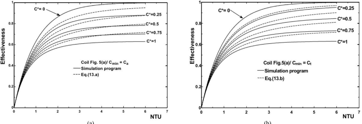
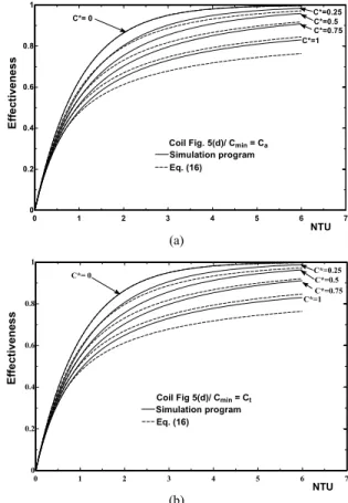
Figures 6 to 9 present the plots of effectiveness versus the Number of Transfer Units for the coils of Fig. 5. Two plots are included in each figure corresponding to either the tube fluid or the air with the lower heat capacity rate. The upper continuous line in each plot corresponds to C* = 0, Eq. (20). For comparison purposes, results from Table 1 correlations have been superposed with those from the program in each plot (broken lines). The correlation from Table 1 used for comparison in each plot is the one with the same number of rows as the corresponding coil in Fig. 5. A close examination of these plots allows one to draw several conclusions, which can be summarized as follows:
(1) For the same value of NTU, the coil effectiveness increases with the number of rows. This is an expected result given that the heat transfer area increases with the number of rows and, as a result, so does the exit temperature of both fluids.
(2) The (ε, NTU) relationship depends on which of the fluids is the one with the lowest heat capacity rate. This trend is clearly reproduced by the correlations of Table 1, and by the simulation program results as plots (a) and (b) differ from each other.
Figure 5. Tube fluid flow arrangement of the coils. The air flows from left to right. (a) Z-shape cross-flow Nt = 12; (b) staggered row and two-circuit arrangement, Nt = 10; (c) staggered three-row two-two-circuit arrangement, Nt = 10; (d) staggered six-row five-circuit arrangement, Nt = 10.
(4) As a general rule, in the range of higher NTU (roughly NTU>1.5), the correlations tend to underestimate the coil effectiveness. An exception to this rule is the geometry of Fig. 5(a), since, in this case, Eqs. 13(a) and (b), for two row coils, over-predict the effectiveness.
(5) In the range of lower NTU, correlations results with respect to those from the simulation program do not follow a clear trend, and the relative behavior depends on the particular geometry and flow arrangement. For example, in the case of the geometry of Fig. 5(d), for both conditions of lower heat capacity rate, Figs. 9(a) and (b) clearly display a trend shift in the relative behavior of the (ε, NTU) relationship. In fact, in the lower NTU range, the correlation effectiveness slightly overestimates the simulation program. This trend changes for higher NTU values, with the shifting point depending on the heat capacity ratio. The lower the latter, the higher the shifting NTU. Notice that the same conclusion applies to Figs. 7 and 8 and the shift point behavior is also the same.
(6) Deviations of correlation with respect to program results are presented in Table 4, reaching values as high as 12.0%, obtained for the coil of Fig. 5(a). Deviations for the other coils are limited to a maximum of 8.39% for the Fig. 5(d) coil. The
least deviations occur for the coil of Fig. 5(b), with two parallel tube fluid circuits.
(7) The deviations for cases (a) and (b) of the plots of Figs. 6 to 9 tend to be very close to each other.
(8) It is interesting to note, as clearly shown in Table 4, that the maximum deviations occur preferably for a heat capacity ratio of the order of one, and relatively high NTU values (of the order of 5). An exception to this rule is the geometry of Fig. 5(b), which coincidently is the one with lower deviations. In this case, the maximum deviation is obtained at a heat capacity ratio of 0.1 and a NTU equal to 0.1.
(9) A comparison of the Stevens et al. (1957) correlation results, Eq. (16), with those from the simulation program, for the coil of Fig. 5(d), has also been included in the last row of Table 4. Deviations are similar to those obtained for the ESDU (1998) correlation, Eq. (17). The maximum deviation of results from these correlations with respect to those from the simulation program are of the order of 8%, a value that makes their use questionable for coils with this flow arrangement and number of tube rows.
Table 4. Deviations of correlations from Table 1 with respect to simulation program results for the coils of Fig. 5.
Average relative error , %, maximum relative error, % (C*, NTU)* Coil Equation
Cmin= Cair, kW/K Cmin= Ct, kW/K Fig. 5(a) 13 (a) and (b) 6.40, 12.02, (0.9, 6) 4.49, 11.93, (1, 6) Fig. 5(b) 13 (a) and (b) 2.08, 4.61, (0.1, 0.1) 2.14, 4.52, (0.1, 0.1) Fig. 5(c) 14 (a) and (b) 3.12, 6.29, (1, 5.1) 3.18, 6.29, (1, 5.1)
Fig. 5(d) 17 3.29, 8.31, (1, 6) 3.45, 8.39, (0.9, 6)
Fig. 5(d) 16 3.67, 7.81, (1, 4.6) 3.86, 7.81, (1, 4.6) * C* and NTU corresponding to the maximum deviation.
0 1 2 3 4 5 6 7
0 0.2 0.4 0.6 0.8 1
NTU
Simulationprogram
Simulationprogram
Eq.(13.a)
Eq.(13.a)
C*=1
CoilFig.5(a)/Cmin=Ca
C*=0.75 C*=0.5 C*=0.25
C*=0
Effecti
v
eness
0 1 2 3 4 5 6 7
0 0.2 0.4 0.6 0.8 1
NTU
Simulationprogram Simulationprogram Eq.(13.b) Eq.(13.b)
C*=1
Coil Fig.5(a)/Cmin=Ct
C*=0.75 C*=0.5 C*=0.25 C*= 0
Effecti
ven
ess
(a) (b)
0 1 2 3 4 5 6 7 0
0.2 0.4 0.6 0.8 1
NTU
Simulation program Simulation program Eq. (13.a) Eq. (13.a)
C*=1
Coil Fig.5(b)/ Cmin = Ca
C*=0.75 C*=0.5 C*=0.25
Effecti
v
en
es
s
C*= 0
(a)
0 1 2 3 4 5 6 7
0 0.2 0.4 0.6 0.8 1
NTU
Simulation program Simulation program Eq. (13.b) Eq. (13.b)
C*=1
Coil Fig. 5(b)/ Cmin = Ct
C*=0.75 C*=0.5 C*=0.25
E
ffe
ct
iv
e
n
es
s
C*= 0
(b)
Figure 7. Effectiveness variation with NTU for the coil of Fig. 5(b). Correlation results are plotted as broken lines (two rows). (a) Ca < Ct; (b) Ct < Ca.
0 1 2 3 4 5 6 7
0 0.2 0.4 0.6 0.8 1
NTU
Simulationprogram
Simulationprogram
Eq.(14.a)
Eq.(14.a)
C*=1
CoilFig.5(c)/Cmin=Ca
C*=0.75 C*=0.5 C*=0.25 C*=0
E
ffecti
venes
s
(a)
0 1 2 3 4 5 6 7
0 0.2 0.4 0.6 0.8 1
NTU
Simulationprogram
Simulationprogram
Eq.(14.b)
Eq.(14.b)
C*=1
CoilFig.5(c)/Cmin=Ct
C*=0.75 C*=0.5 C*=0.25 C*=0
E
ffec
tiv
en
es
s
(b)
Figure 8. Effectiveness variation with NTU for the coil of Fig. 5(c). Correlation results are plotted as broken lines (three rows). (a) Ca < Ct; (b) Ct < Ca.
0 1 2 3 4 5 6 7
0 0.2 0.4 0.6 0.8 1
NTU
Simulation program Simulation program Eq. (16) Eq. (16)
C*=1
Coil Fig. 5(d)/ Cmin = Ca
C*=0.75 C*=0.5 C*=0.25
Eff
ec
ti
v
en
ess
C*= 0
(a)
0 1 2 3 4 5 6 7
0 0.2 0.4 0.6 0.8 1
NTU
Simulation program Simulation program Eq. (16) Eq. (16)
C*=1
Coil Fig 5(d)/ Cmin = Ct
C*=0.75 C*=0.5 C*=0.25
Effe
c
tiv
en
es
s
C*= 0
(b)
Figure 9. Effectiveness variation with NTU for the coil of Fig. 5(d). Correlation results are plotted as broken lines (six rows). (a) Ca < Ct; (b) Ct < Ca.
Conclusions
The computer simulation program described herein has been applied in the evaluation of (ε, NTU) relationships for air conditioning and refrigeration coils. It has been determined that, for the case of strictly cross-flow geometries, the available (ε, NTU) correlations are adequate up to four tube rows. Correlations for an infinite number of tube rows, such as the Stevens et al. (1957), are relatively inaccurate when applied to coils with rows varying in the range between 5 and 10. Caution must be exercised when applying (ε, NTU) closed form correlations to complex flow arrangement and geometry coils, since it has been shown that moderate inaccuracies might result. In such cases, the use of simulation programs like the one of the present paper is recommended.
As a concluding remark, it must be stressed that the results discussed herein regarding coils of complex geometry allow one to conclude that the indiscriminate use of closed form correlations could lead to unacceptable inaccuracies in the determination of either the effectiveness or the NTU. An example of the latter would be the case when air-side heat transfer data are being determined from experiments involving flow of water inside the tubes. Since the tube-side heat transfer characteristics are readily known, the air-side ones are obtained from the overall coil conductance (UA), which in turn results from the (ε, NTU) relationship. Thus, NTU inaccuracies could cause same order inaccuracies in the air-side heat transfer characteristics.
Acknowledgements
Desenvolvimento Científico). The second author thanks CNPq and FAPEMIG (Fundação de Amparo à Pesquisa do Estado de Minas Gerais). G. Ribatski acknowledges the support given by The State of São Paulo Research Foundation – FAPESP, Brazil.
References
Baclic, B.S., 1990, “ε-NTU analysis of complicated flow arrangements”. In: R.K. Shah, A.D. Kraus, and D. Metzger (editors) “Compact Heat Exchangers”. Hemisphere Publishing, New York, pp.31-90.
Bansal, P.K. and Purkayastha, B., 1998, “An NTU-ε model for alternative refrigerants”, International Journal of Refrigeration, Vol. 21, No. 5, pp. 381-397.
Bensafi, A., Borgand, S. and Parent, D., 1997, “CYRANO: a computational model for the detailed design of plate-fin-and-tube heat exchangers using pure and mixed refrigerants”, International Journal of Refrigeration, Vol. 20, No. 3, pp. 218-238.
Bowman, R.A., Mueller, A.C. and Nagle, W.M., 1940, “Mean temperature difference in design”, ASME Transactions, Vol. 62, pp. 283-293.
Cabezas-Gómez, L., Navarro, H.A. and Saiz-Jabardo, J.M., 2007, “Thermal performance of multi-pass parallel and counter cross-flow heat exchangers”, ASME Heat and Mass Transfer (in press).
Corberán, J.M. and Melón, M.G., 1998, “Modelling of plate finned tube evaporators and condensers working with R134a”, International Journal of Refrigeration, Vol. 21, No. 4, pp. 273-284.
Domanski, P.A., 1991, “Simulation of an evaporator with non-uniform one-dimensional air distribution”, ASHRAE Transactions, Vol. 97, No. 1, pp. 793-802.
Domingos, J.D., 1969, “Analysis of complex assemblies of heat exchangers”, International Journal of Heat and Mass Transfer, Vol. 12, pp. 537-548.
ESDU 98005, 1998, “Design and Performance Evaluation of Heat Exchangers: The Effectiveness – NTU Method”. Engineering Science Data Unit 98005, London: ESDU International Publishing, July, pp. 46-61.
Kays, W.M. and London, A.L., 1998, “Compact Heat Exchangers”. New York: McGraw-Hill.
Mason, J.L., 1955, “Heat transfer in crossflow”, Proceedings 2nd US National Congress of Applied Mechanics, ASME, New York, pp. 801-803.
Navarro, H.A. and Cabezas-Gómez, L., 2005, “A new approach for thermal performance calculation of cross-flow heat exchangers”,
International Journal of Heat Mass Transfer, Vol. 48, pp. 3880-3888. Pignotti, A., 1988, “Linear matrix operator formalism for basic heat exchanger thermal design”, ASME Journal of Heat Transfer, Vol. 110, pp. 297-303.
Pignotti, A and Shah, R.K., 1992, “Effectiveness-number of transfer units relationships for heat exchanger complex flow arrangements”,
International Journal of Heat and Mass Transfer, Vol. 35, pp. 1275-1291. Pignotti, A. and Cordero, G.O., 1983, “Mean temperature difference in multipass crossflow”, ASME Journal of Heat Transfer, Vol. 105, pp. 592-597.
Rich, D.G., 1975, “The effect of the number of tube rows on heat transfer performance of smooth plate fin-and-tube heat exchangers”,
ASHRAE Transactions, Vol. 81, pp. 307-319.
Shah, R.K. and Pignotti, A., 1993, “Thermal analysis of complex crossflow exchangers in terms of standard configurations”, ASME Journal of Heat Transfer, Vol. 115, pp. 353-359.
Stevens, R.A., Fernandez, J. and Woolf, J.R., 1957, “Mean temperature difference in one, two and three-pass crossflow heat exchangers”,
Transactions ASME, Vol. 79, pp. 287-297.
Vardhan, A. and Dhar, P.L., 1998, “A new procedure for performance prediction of air conditioning coils”, International Journal of Refrigeration, Vol. 21, No. 1, pp. 77-83.