J. Braz. Soc. Mech. Sci. & Eng. vol.32 número4

Cristiano V. da Silva

cristiano@uricer.edu.br Universidade Regional Integrada do Alto Uruguai e das Missões – URI Campus de Erechim Department of Eng. and Computational Science GEAPI – Group of Applied Engineering to Industrial Processes LABSIM – Numerical Simulation Laboratory 99700-000 Erechim, RS, Brazil

Maria Luiza S. Indrusiak

sperbindrusiak@via-rs.net UNISINOS – Universidade do Vale do Rio dos Sinos Graduate Program in Mechanical Engineering 93022-000 São Leopoldo, RS, Brazil

Arthur B. Beskow

Arthur@uricer.edu.br Universidade Regional Integrada do Alto Uruguai e das Missões – URI Campus de Erechim Department of Eng. and Computational Science GEAPI – Group of Applied Engineering to Industrial Processes LABSIM – Numerical Simulation Laboratory 99700-000 Erechim, RS, Brazil

CFD Analysis of the Pulverized Coal

Combustion Processes in a 160 MWe

Tangentially-Fired-Boiler of a Thermal

Power Plant

The strategic role of energy and the current concern with greenhouse effects, energetic and exergetic efficiency of fossil fuel combustion greatly enhance the importance of the studies of complex physical and chemical processes occurring inside boilers of thermal power plants. The state of the art in computational fluid dynamics and the availability of commercial codes encourage numeric studies of the combustion processes. In the present work the commercial software CFX © Ansys Europe Ltd. was used to study the combustion of coal in a 160 MWe commercial thermal power plant with the objective of simulating the operational conditions and identifying factors of inefficiency. The behavior of the flow of air and pulverized coal through the burners was analyzed, and the three-dimensional flue gas flow through the combustion chamber and heat exchangers was reproduced in the numeric simulation.

Keywords: coal combustion, computational fluid dynamics, thermal power plant

Introduction

1

In many parts of the world, coal is an important energy resource to meet the future demand for electricity, as coal reserves are much greater than for other fossil fuels. However, the efficient and clean utilization of this fuel is a major problem in combustion processes. In recent years, the interest on performance optimization of large utility boilers has become very relevant, aiming at extending their lifetime, increasing the thermal efficiency and reducing the pollutant emissions, particularly the NOx emissions.

Coal reserves in Brazil, which are used mainly for electricity production in large utility boilers, are enough to meet the next 1,109 years demand, considering the consumption levels of 2006 (EIA/U.S. Department of Energy, 2009). Nonetheless, in order to face the competition from renewable, natural gas and nuclear energy sources, some main problems must be solved, as to reduce CO2

emissions through increasing efficiency (Williams et al., 2000). Also NOx and SOx emissions should be reduced to environmentally

acceptable levels. An efficient operation of combustion chambers of these boilers depends on the proper knowledge of the oxidation reactions and heat transfer between the combustion products and the chamber walls and heat exchangers, which requires a detailed analysis of the governing mechanisms. Many combustion modeling methodologies are now available, but only a few are able to deal with the process in its entirety. Eaton et al. (1999) present a revision of combustion models. The models are generally based on the fundamental conservation equations of mass, energy, chemical species and momentum, while the closure problem is solved by turbulence models such as the k−

ε

(Launder and Sharma, 1974),

Paper accepted February, 2010. Technical Editor: Demétrio Bastos Neto.

combustion models like Arrhenius (Kuo, 1996; Turns, 2000), Magnussen – EBU – “Eddy Breakup” (Magnussen and Hjertager, 1976); radiative transfer models based on the Radiative Transfer Equation – RTE (Carvalho et al., 1991) and models to devolatilization and combustion of solid and liquid fuels.

Abbas et al. (1993) describe an experimental and predicted assessment of the influence of coal particle size on the formation of NOx of a swirl-stabilized burner in a large-scale laboratory furnace.

Three particle size distributions, 25, 46, and 121 μm average size, of high volatile coal were fired under similar operation conditions. The data presented combine detailed in-flame measurements of gas temperature, gas species concentrations of CO, CH4, O2, NOx, HCL,

NH3, particle burnout, and “on-line” N2O, with the complementary

predicted studies. The predicted results are in good agreement with experimental data. Although the NOx emission trends with particle

size are similar, predicted values for each fraction are higher, suggesting a limitation in the NOx reducing mechanisms used in the

model. Three mechanisms – thermal, fuel and prompt – were used to calculate the NOx formation.

Xu et al. (2000) employed the CFD code to analyze a coal combustion process in a front wall pulverized coal fired utility boiler of 350 MW with 24 swirl burners installed at the furnace front wall. Five different cases with 100, 95, 85, 70 and 50% boiler full load were simulated. Comparisons were addressed, with good agreement between predicted and measured results in the boiler for all but one case thus validating the models and the algorithm employed in the computation.

p

k

k

−

ε

−

two-phase turbulence model and a second-order-moment (SOM) reactive rate model were proposed. The proposed models were used to simulate NOx formation of methane-air

combustion, and the prediction results were compared with those using only the presumed-PDF (Probability Density Function)-finite-reaction-rate model and experimental data. The proposed models were also used to predict the coal combustion and NOx formation at

the exit of a double air register swirl pulverized-coal burner. The results indicate that a pulverized coal concentrator installed in the primary air tube of the burner has a strong effect on the coal combustion and NOx formation.

In a numerical investigation, Kurose et al. (2004) employed a tree-dimensional simulation to the pulverized coal combustion field in a furnace equipped with a low-NOx burner, called CI-α, to

investigate in details the combustion processes. The validities of available NOx formation and reduction models were investigated

too. The results show that a recirculation flow is formed in high-gas-temperature region near the CI-α burner outlet, and this lengthens the residence time of coal particles in this high-gas-temperature region, promotes the evolution of volatile matter and the process of char reaction, and produces an extremely low-O2 region for effective

NO reduction.

Zhang et al. (2005) presented a numerical investigation on the coal combustion process using an algebraic unified second-order moment (AUSM) turbulence-chemistry model to calculate the effect of particle temperature fluctuation on char combustion. The AUSM model was used to simulate gas-particles flows in coal combustion including sub-models as the

k

−

ε

−

k

_p two-phase turbulence model, the EBU-Arrhenius volatile and CO combustion model, and the six-flux radiation model. The simulation results indicate that the AUSM char combustion model presented good result, since the latter totally eliminates the influence of particle temperature fluctuation on char combustion rate.

Bosoaga et al. (2006) presented a study developing a CFD model for the combustion of low-grade lignite and to characterize the combustion process in the test furnace, including the influence of the geometry of burner and furnace. A number of computations were made in order to predict the effect of coal particle size, the moisture content of lignite, and the influence of combustion temperature and operation of the support methane flame on the furnace performance and emissions. The influence of lignite pre-drying was also modeled to investigate the effects of reduced fuel consumption and CO2 emissions. It was found that the increase of

moisture tends to reduce NOx, and the methane support flame

greatly increases NOx.

In another work, Backreedy et al. (2006) presented a numerical and experimental investigation of the coal combustion process to predict the combustion process of pulverized coal in a 1 MW test furnace. The furnace contains a triple-staged low-NOx swirl burner.

A number of simulations were made using several coal types in order to calculate NOx and the unburned carbon-in-ash, the latter

being a sensitive test for the accuracy of the char combustion model. The NOx modeling incorporates fuel-NO, thermal, and prompt

mechanisms to predict the NO formation on the combustion processes.

Kumar and Sahur (2007) studied the effect of the tilt angle of the burners in a tangentially fired 210 MWe boiler, using commercial code FLUENT. They showed the influence of the tilt angle in the residence time of the coal particles and consequently in the temperature profiles along the boiler.

Asotani et al. (2008), also using the code FLUENT, studied the ignition behavior of pulverized coal clouds in a 40 MW commercial tangentially fired boiler. The results for unburned carbon in ash and for outlet temperature were validated respectively by the operating

data and by the design parameter. A qualitative comparison between the results for temperature and ignition behavior in the vicinity of the burners was made, using the images of a high temperature resistant video camera system. At the same line Choi and Kim (2009), also using the code FLUENT, investigated numerically the characteristics of flow, combustion and NOx emissions in a 500 MWe tangentially fired pulverized-coal boiler. They showed that the relation among temperature, O2 mass

fraction and CO2 mass fraction has been clearly demonstrated

based on the calculated distributions, and the predicted results have shown that the NOx formation in the boiler highly depend on

the combustion process as well as the temperature and species concentration.

The strategic role of energy and the current concern with greenhouse effects enhance the importance of the studies of complex physical and chemical processes occurring inside boilers of thermal power plants. Combustion comprises phenomena such as turbulence, radiative and convective heat transfer, particle transport and chemical reactions. The study of these coupled phenomena is a challenging issue. The state of the art in computational fluid dynamics and the availability of commercial codes encourage numeric studies of the combustion processes. In the present work, a commercial CFD code, CFX © Ansys Europe Ltd., was used to study the pulverized-coal combustion process in a 160 MWe thermal power plant erected in the core of the Brazilian coal reserves region, with the objective of simulating the operation conditions and identifying inefficiency factors.

Nomenclature

x

NO = Oxides of nitrogen

4

CH = Methane

2

O = Oxygen

2

N = Nitrogen

2

CO = Carbon dioxide

CO = Carbon monoxide O

H₂ = Water vapor

3

NH = Ammonia

k = Constant of chemical reaction rate; or turbulent kinetic energy, m2/s2

x = Spatial coordinate, m r = Vector position, m

s

= Vector direction, m

"

S = Radiation source term, W/m

α

K = Absorption coefficient, m-1

~

U = Average velocity, m/s Sc = Schmidt number

μ

C = Empirical turbulence model constant

o

C = Mass fraction of raw coal, kg/kg

ch

C = Mass fraction of char, kg/kg

*

p = Modified pressure, Pa

A

p = Atmospheric pressure, Pa

p = Average pressure, Pa D = Dynamic mass diffusivity, m2/s

~

Y = Average mass fraction kg/kg

1

Y = First reaction

2

I = Total radiation intensity, W/m2

R = Chemical reaction rate, kg/(s.m3) or rate of formation/destruction of chemical species, W/m3_.kg

ℜ = Universal ideal gas constant 8314.5 kJ/(kmol K) E = Activation energy, J/kmol

A = Empirical coefficient, (m3/s)/kmol

~

C = Average molar concentration, kmol/m3

MM = Molecular mass, kg /kmol

1

K = Empirical constant

2

K = Empirical constant

~

h = Average enthalpy of mixture, kJ/kg 0

ref

h = Enthalpy of formation, kJ/kg

t

= Time, s

p

c = Specific heat, kJ/(kg.K)

S = Path length, m; or source term, W/m3

Greek Symbols

k

σ = Prandtl number

ϖ

σ = Prandtl number

w

τ = Shear stress in the wall, Pa ρ = Density, kg/m3

μ = Dynamic viscosity, (N.s)/m2

ε = Dissipation of turbulent kinetic energy, m2/s3 β = Temperature exponent or empirical constant

'

β = Empirical constant

α = Empirical constant or α-th chemical species Π = Product symbol

γ = Concentration exponent η = Stoichiometric coefficient, kmol κ = Thermal conductivity, W/(m.K)

σ = Stefan-Boltzmann constant, 5.678x10-8 W/(m2.K4) δ = Krönecker delta function

Subscripts

j Index

i Index or Chemical species k Chemical reaction or index t Turbulent

rad Radiation rea Chemical reaction g Gas

s Surface

d Oxygen diffusion o Raw coal

c

Char ref Reference

p Products or particles eff Effective

Superscripts

* Represents the

α

-reacting component that leads to the smallest value for R

p Represents the combustion gas products

Mathematical Formulation

A steady-state combustion of raw coal in air for a boiler combustion chamber is considered in order to determine the temperature, chemical species concentrations and the velocity fields for multi-component-flow (gas mixture and raw coal particles), as well as to study the influence of the operational parameters, such as heterogeneous condition for fuel and air flow in the chamber, on the combustion process and NOx formation.

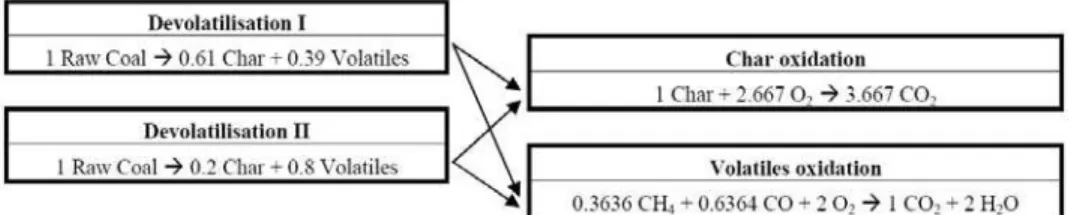
The complete chemical reaction of the raw coal used at this work, including two devolatilization processes, is modeled according to the basic scheme showed in Fig. 1.

As basic assumptions, it is considered that the mass fractions of volatiles are 0.3636 of methane and 0.6364 of carbon monoxide, and that the combustion processes of these volatiles occur at finite rates. The methane oxidation is modeled by two global steps, given by:

(

( ) ( )

)

( ) ( ) ( )

) (

N . O H CO N

. O

CH416 3 232 376 228 2 28 4 2 18 1128 228

2 + + → + + (1)

(

( ) ( )

)

( ) ( )

)

( _{O . N CO . N}

CO28 1 ₂32 376 ₂28 2 ₂28 376 ₂28

2 + + → + (2)

Equation 2 also models the combustion of carbon monoxide resulting from the devolatilisation processes. The formation of NOx

is modeled using two different paths, the thermal-NO (Zeldovich mechanism) and the prompt-NO (Fennimore mechanism), where the first, predominant at temperatures above 1800 K, is given by tree-step chemical reaction mechanisms (CFX Inc., 2004):

) ( ) ( ) ( )

( _{N NO N}

O16 + ₂28 → 30 + 14 (3)

) ( ) ( ) ( ) (

O NO O

N14 + 232 → 30 + 16 (4)

In sub or near stoichiometric conditions, a third reaction is also used:

) ( ) ( ) ( ) (

H NO N

OH17 + 14 → 30 + 1 (5)

where the chemical reaction rates are predicted by Arrhenius equation.

For the prompt-NO, formed at temperatures lower than 1800 K, radicals can react with molecular nitrogen to form HCN, which may be oxidized to NO under flame conditions. The complete mechanism is not straightforward. However, De Soete proposed a single reaction rate to describe the NO source by Fennimore mechanism, which is used at this work. Arrhenius equations are used for predicting this chemical reaction rate (CFX Inc., 2004).

For multi-component-fluid, scalar transport equations are solved for velocity, pressure, temperature and chemical species. Additional equations are solved to determine how the components of the fluid are transported within the fluid. The bulk motion of the fluid is modeled using single velocity, pressure, temperature, chemical species and turbulence intensity fields.

Mass and Species Conservation

Each component has its own Reynolds-Averaged equation for mass conservation which, considering incompressible and stationary flow can be written in tensor notation as:

i j i ~ j ~ ij ~

i ~

j j

~ j i ~

S " U " U U x x

U

+ ⎟ ⎟ ⎠ ⎞ ⎜

⎜ ⎝ ⎛

− ⎟⎟ ⎠ ⎞ ⎜⎜

⎝ ⎛

− ∂

∂ = ∂

⎟⎟ ⎠ ⎞ ⎜⎜ ⎝ ⎛ ∂

ρ ρ

ρ

where _{∑ ρ ⎟⎟ ρ} ⎠ ⎞ ⎜⎜ ⎝ ⎛ = ij ~ i ~ j ~ U U . ~ i

ρ and ρ are the mass-average density of

fluid component

i

in the mixture and average density, respectively,

x

is the spatial coordinate,

~

U is the vector of velocity and

~ ij

U

is

the mass-averaged velocity of fluid component i. The term

⎟⎟ ⎠ ⎞ ⎜⎜ ⎝ ⎛ − j ~ ij ~ i ~ U U

ρ represents the relative mass flow, and Si is the source

term for component

i

which includes the effects of chemical reactions. Note that if all the equations represented by Eq. (6) are added over all components, and the source term is set to zero, the result is the standard continuity equation.

The relative mass flow term accounts for differential motion of the individual components. At this work, this term is modeled for the relative motion of the mixture components and the primary effect is that of concentration gradient. Therefore,

i ~ i i j ~ ij ~ i ~ x D U U ∂ ∂ = ⎟⎟ ⎠ ⎞ ⎜⎜ ⎝ ⎛ − ρ ρ ρ

ρ (7)

where

D

_i is the kinetic diffusivity. The mass fraction of component

i

is defined as i ρ~_i ρ

~

Y = . Substituting this expression into Eq. (7)

and modeling the turbulent scalar flows using the eddy dissipation assumption, it follows that

i j ~ i t t i j ~ i j ~ j S x Y Sc D x Y U

x _⎟⎟+

⎟ ⎠ ⎞ ⎜ ⎜ ⎜ ⎝ ⎛ ∂ ∂ ⎟⎟ ⎠ ⎞ ⎜⎜ ⎝ ⎛ + ∂ ∂ = ⎟⎟ ⎠ ⎞ ⎜⎜ ⎝ ⎛ ∂

∂ _{ρ ρ} μ

(8)

where

μ

_t is the turbulent viscosity and Sc_t is the turbulent Schmidt number. Note that the sum of component mass fractions over all components is equal to one.

Momentum Conservation

For the fluid flow the momentum conservation equations are given by: U i j ~ j i ~ eff j * j ~ j ~ i j S x x U x U x x p U U

x ∂ ∂ +

∂ + ⎟ ⎟ ⎟ ⎠ ⎞ ⎜ ⎜ ⎜ ⎝ ⎛ ∂ ∂ ∂ ∂ + ∂ ∂ − = ⎟⎟ ⎠ ⎞ ⎜⎜ ⎝ ⎛ ∂

∂ _{ρ δ μ (9)}

where μeff =μ+μt and

μ

is the mixture dynamic viscosity and μt is

the turbulent viscosity, defined as μt=C_μρ k2/ε . The term k

) / ( p

p*= − 2 3 is the modified pressure, C_μ is an empirical constant of the turbulence model and equal to 0.09, p is the time-averaged pressure of the gaseous mixture, and δ is the Krönecker delta function. SU is the source term, introduced to model the buoyancy and drag force due to the transportation particles, and other mathematical terms due to turbulence models. The Boussinesq model is used to represent the buoyancy force due to density variations.

The k−ϖ Turbulence Model

The equations for turbulent kinetic energy, k, and its turbulent frequency,

ϖ

, are (Menter, 1994):

ϖ ρ β σ μ μ

ρ P ' k

x k x

k U

x _{k j} k

t j ~ j j − + ⎟ ⎟ ⎠ ⎞ ⎜ ⎜ ⎝ ⎛ ∂ ∂ ⎟⎟ ⎠ ⎞ ⎜⎜ ⎝ ⎛ + ∂ ∂ = ⎟⎟ ⎠ ⎞ ⎜⎜ ⎝ ⎛ ∂

∂ ₍₁₀₎

2 βρϖ ϖ α ϖ σ μ μ ϖ ρ

ϖ ⎟+ −

⎟ ⎠ ⎞ ⎜ ⎜ ⎝ ⎛ ∂ ∂ ⎟⎟ ⎠ ⎞ ⎜⎜ ⎝ ⎛ + ∂ ∂ = ⎟⎟ ⎠ ⎞ ⎜⎜ ⎝ ⎛ ∂ ∂ k j t j ~ j j P k x x U

x (11)

where β', β and

α

are empirical constants of the turbulence model, σk and σϖ are the Prandtl numbers of the kinetic energy

and frequency, respectively, and

P

_k is the term which accounts for the production or destruction of the turbulent kinetic energy.

⎟ ⎟ ⎠ ⎞ ⎜ ⎜ ⎝ ⎛ ∂ ∂ + ∂ ∂ = i j j i t k x U x U

P μ (12)

Energy Conservation

Considering the transport of energy due to the diffusion of each chemical species, the energy equation can be written as

rea rad Nc i j ~ i i ~ i j ~ t t p j ~ ~ j j S S x Y h D x h Pr c x h U

x _⎟⎟+ +

⎟ ⎠ ⎞ ⎜ ⎜ ⎜ ⎝ ⎛ ∂ ∂ + ∂ ∂ ⎟ ⎟ ⎠ ⎞ ⎜ ⎜ ⎝ ⎛ + ∂ ∂ = ⎟⎟ ⎠ ⎞ ⎜⎜ ⎝ ⎛ ∂

∂ _ρ κ μ

_∑

_ρ

(13)

where

~

h

and

c

p are the average enthalpy and specific heat of the mixture. The latter is given by

∑

=

α α p,α

~

p Y c

c (14)

where c_p,α and

~

Y are the specific heat and the average mass

fraction of the α-th chemical species,

κ

is the thermal conductivity of the mixture, Prt is the turbulent Prandtl number, and Srad and

rea

S represent the sources of thermal energy due to the radiative transfer and to the chemical reactions. The term Srea can be written as:

α α

α α α

α _{c dT R}

MM h S ~ ~ T , ref ~ T , p

rea

∑

∫

⎥ ⎥ ⎥ ⎥ ⎦ ⎤ ⎢ ⎢ ⎢ ⎢ ⎣ ⎡ +

= 0 (15)

where

~

T is the average temperature of the mixture, h_α0 and ref,α ~

T are the formation enthalpy and the reference temperature of the α-th chemical species. To complete the model, the density of mixture can be obtained from the ideal gas state equation (Kuo, 1996; Spalding,

1979; Turns, 2000), −1

⎟⎟ ⎠ ⎞ ⎜⎜ ⎝ ⎛ ℜ

=pMM T~

ρ , where

p

is the combustion

chamber operational pressure, which is here set equal to 1 atm (Spalding, 1979), and MM is the mixture molecular mass. The aforementioned equations are valid only in the turbulent core, where

μ

μ >>t . Close to the wall, the logarithmic law of the wall is used.

inside the combustion chamber and its value is 0.5 m-1. Then, the Radiative Transfer Equation – RTE is integrated within its spectral band and a modified RTE can be written as

( )

_{( )}

"

a ~

a T _{K I r,s S}

K dS

s , r

dI _{= − +}

π σ 4

(16)

At the equation above, σ is the Stefan-Boltzmann constant (5.672 x 10-8 W/m2K4),

r

is the vector position,

s

is the vector direction, S is the path length, Ka is the absorption coefficient,

I is the total radiation intensity which depends on position and direction, and S" is the radiation source term, where the radiative emission of the solid particles can be computed. The radiative properties required for an entrained particle phase are the absorption coefficients and scattering phase function, which depend on the particle concentration, size distribution, and effective complex refractive indices. However, optical properties of coal are not well characterized (Eaton et al., 1999). Generally, as a starting point to arrive at a tractable method for calculating radiative properties, the particles are assumed to be spherical and homogeneous. At this work, the heat transfer from gas mixture to particle considers that the particles are opaque bodies with emissivity equal to one, and the Hanz-Marshall correlation is used to model the heat transfer coupling between the gas mixture flow and the particles (CFX Inc., 2004).

The E-A (Eddy Breakup – Arrhenius) Chemical Reactions Model

The reduced chemical reactions model employed in this work assumes finite rate reactions and a steady state turbulent process to volatiles combustion. In addition, it is considered that the combined pre-mixed and non-premixed oxidation occurs in two global chemical reaction steps, and involving only six species: oxygen, methane, nitrogen, water vapor, carbon dioxide and carbon monoxide. A conservation equation is required for each species but nitrogen. Thus, one has the conservation equation for the α-th chemical species, given by Eq. (8), where the source term, Si,

considers the average volumetric rate of formation or destruction of the α-th chemical species at all chemical reactions. This term is computed from the summation of the volumetric rates of formation or destruction in all the k-th equations where the α-th species are

present, Rα,k . Thus, =

∑

k

k ,

R R_{α α} .

The rate of formation or destruction, Rα,k, can be obtained

from an Arrhenius kinetic rate relation, which takes into account the turbulence effect, such as Magnussen equations (Eddy Breakup) (Magnussen and Hjertager, 1976), or a combination of the two formulations, the so called Arrhenius-Magnussen model (Eaton et al., 1999; CFX Inc., 2004). Such relations are appropriate for a wide range of applications, for instance, laminar or turbulent chemical reactions with or without pre-mixing. The Arrhenius equation can be written as follows:

⎟⎟ ⎟ ⎠ ⎞ ⎜⎜ ⎜ ⎝ ⎛

ℜ − −

= ~ ,k _~k

k k ~ k , Chemical , k ,

T E exp C A T MM R

α γ α α β α α

α η Π (17)

where β_k is the temperature exponent in each chemical reaction k, which is obtained empirically together with the energy activation

k

E and the coefficient Ak. Πα is the product symbol, α

~

C

is the

molar concentration of the α-th chemical species, γα,k is the

concentration exponent in each reaction k, ℜ is the gas constant,

α

MM and ηα,k are the molecular mass and the stoichiometric

coefficient of

α

in the

k

-th chemical reaction.

In the Eddy-Breakup or Magnussen model, the chemical reaction rates are based on the theories of vortex dissipation in the presence of turbulence. Thus, for diffusive flames:

* k , *

* ~

k , EBU , k ,

MM Y k A MM R

α α

α α

α α

η ε ρ η

−

= (18)

where the index α* represents the reactant

α

that has the least value of R_α,k,EBU .

In the presence of premixing, a third relation for the Eddy Breakup model is necessary, so that

∑

∑

=

p

p k , p

p p ~

k , emixing ,Pr k ,

MM Y

k AB MM R

η ε ρ

ηα α

α (19)

where the index p represents the gaseous products of the combustion. A and B are empirical constants that are set as 4 and 0.5 (Magnussen and Hjertager, 1976). Magnussen model, Eqs. (18) and (19), can be applied to both diffusive and pre-mixed flames, or for the situation where both flames coexist, taking the smallest rate of chemical reaction.

Finally, for the Arrhenius-Magnussen model, given by Eqs. (17), (18) and (19), the rate of formation or destruction of the chemical species is taken as the lowest one between the values obtained from each model. It follows that Silva et al. (2007) used this formulation in this work to simulate the combustion process of methane and air in a cylindrical chamber obtaining good results. At this way:

(

,k,Chemical ,k,EBU ,k,Premixed

)

k

, min R ,R ,R

R_α = _{α α α} (20)

The Coal Decomposition

Figure 1. Basic scheme of the full chemical reactions of the raw coal.

The Coal Devolatilization Model

The devolatilization of the coal is modeled using the generic Arrhenius reactions capability in two steps (Ubhayakar et al., 1976) in which two reactions with different rate parameters and volatiles yields compete to pyrolyse the raw coal. The first reaction dominates at lower particle temperatures and has a yield Y1 lower

than the yield Y2 of the second reaction which dominates at higher temperatures. As a result, the final yields of volatiles will depend on the temperature history of the particle, and will increase with temperature, lying somewhere between Y1 and Y2. In this model, the mass fraction of the raw coal is specified as the mass fraction of volatiles (here methane and carbon monoxide, see Fig. 1) since all this material could be converted to volatiles.

At time t, it is assumed that a coal particle consists of mass of raw coal (CO), mass of residual char (Cch) after devolatilization

has occurred, and mass of ash (A). The rate constants k1 and k2 of two reactions determine the rate of conversion of the raw coal:

(

)

O

O _{k k C}

dt dC

2 1+ −

= (21)

the rate of volatiles production is given by

(

Yk Y k

)

CO

dt dV

2 2 1 1 +

= (22)

and so the rate of char formation is

(

) (

)

(

)

O

ch _{Y k Y k C}

dt dC

2 2 1

1 1

1− + −

= (23)

The Field Char Oxidation Model

The oxygen diffusion rate is given by k_d

(

p_g−p_S

)

, where pg is

the partial pressure of oxygen in the furnace gases far from particle boundary layer and p_S is the oxygen pressure at the particle surface.

The value of k_d is given by

(

)

p p T

T T R D

k ref A

~ g p p ref d

α

⎟⎟ ⎠ ⎞ ⎜⎜

⎝ ⎛

−

= −1 −1

2 , (24)

where

p

R is the particle radius, T_p is the particle temperature, T~g

is the far-field gas temperature, p_A is atmospheric pressure, D_ref is

the dynamic diffusivity, and α is the exponent with value 0.75. The char oxidation rate per unit area of particle surface is given by k_cp_s. The chemical rate coefficient is given by,

(

c p

)

c

c A exp T T

k = − (25)

where the parameters A_c and T_c depend on the type of coal. The overall char reaction rate of a particle is given by

(

kd kc

)

CO Rp p pA

2 2 1 1 1

4π

− −

− ₊

(26)

and is controlled by the smallest of the two rates, k_d and kc.

Boiler Description

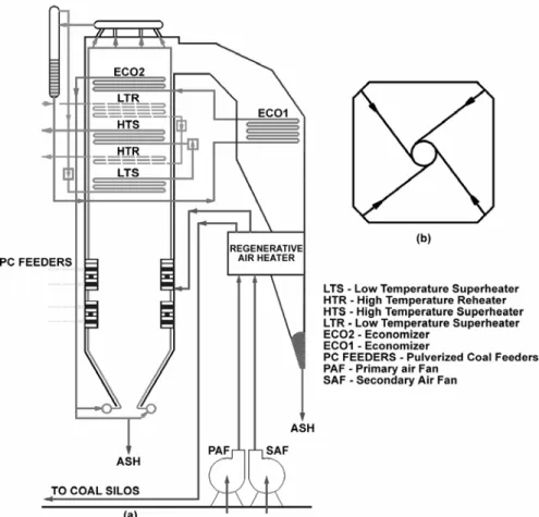
Figure 2. (a) General disposition of the boiler components; (b) Horizontal cross section.

Mesh Settings and Convergence Criteria

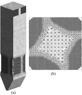
The domain under consideration comprises the first stage of the boiler: the combustion chamber with the burners at the corners and the heat exchangers until the top. The entrance to the second stage was considered the outlet of the domain. The discretization was done using tetrahedral volumes, and the grid details are depicted in Fig. 3. Other type of mesh volumes were not used due to software license limitations. As the boiler height corresponds to only six equivalent diameters of the boiler, the boundary layer is not developed at the whole domain. Nevertheless, prismatic volumes were used at the walls in order to capture the boundary layer behavior. Due to computational limitations, the mesh size used has approximately 1.5 × 106 elements, using mesh refinements in the combustion reactions zone. The convergence criterion adopted was the RMS – root mean square of the residual values, and the value adopted was 1 × 10-6 for all equations.

Boundary Conditions

The boundary conditions were obtained from the design data set and also from the daily operation data sheets. The operating conditions considered were the rated ones, for 160 MW. The following parameters were considered:

Inlet: The inlet conditions are those for air and coal flows entering the domain from the burner nozzles. Total primary and secondary combustion air and pulverized coal mass flow rates were set as 79.5 kg/s, 100 kg/s and 50 kg/s respectively. Temperatures of primary air and coal, and secondary combustion air were set as 542 K and 600 K respectively. Pulverized coal size was modeled by a probabilistic distribution and limited between 50 μm and 200 μm.

Outlet: The outlet boundary is the flue gas passage at lateral wall near the top of the boiler, just above the ECO 2 heat exchanger, where the mean static pressure was. The outlet region was considered as black body to thermal radiation.

Boiler walls: The boiler walls are covered with slanting tubes from the bottom until the beginning of the heat exchangers region. From there to the top the tubes are vertically positioned. Wall roughness to steel was used, and the temperature was set as 673 K, the water saturation temperature at the working pressure of the boiler. The thermal radiation coefficient set for that two wall regions was 0.6.

Results

The temperature field is shown at Fig. 4(b) for a vertical plane diagonally positioned. The large amount of heat released by the devolatilization and oxidation of the volatiles is pointed up by the near black regions at the edge of the flames originated at each burner. Devolatilization is the first reaction of the combustion process and takes place where the air and coal mixture injected by the burners achieve the adequate temperature. The central vortex created by the tangential layout of the burners is visible at the center of the combustion chamber.

the absence of new inflows and the strong turbulence and vorticity of the flow. The velocity fields, Figs. 4(m) to 4(q), represented by means of vectors, show that at the lower burner level the vortex region is narrow and increases in the upstream direction, due to the vorticity moment imparted by the burners jets at each level. Figure 4(m) shows the final aspect of the vortex which dominates the section, with a characteristic dimension of the same magnitude of the boiler wall horizontal length.

There is an intense formation of volatiles very near to the burner nozzles, denoting the action of the first reaction which is activated at relatively low temperatures. The oxidation of the resulting volatile yields is almost immediate, according to the set of equations which models the combustion process.

Figures 4(c) to 4(g) show the distribution of NOx mass

concentration along the boiler. The NOx formation takes place

mainly after the coal devolatilization and volatile oxidation, at the top edges of the air-fuel jets from each burner, where the higher temperatures were achieved. The major role of high temperature along with high oxygen concentration levels in NOx formation is

also emphasized by the impressive enlargement of NOx production

at the higher burner levels. An enhancement of the oxygen concentration is expected at these levels, where the inlet air jets are reinforced by the residual oxygen of the lower levels.

Figure 3. Grid details: (a) At the cross-sections under burner lines; (b) At horizontal cross section in the reactive zone (burners level).

Figure 4. (a) NOx mass fraction; (b) Temperature fields; (c) to (g): NOx mass fraction field, at horizontal planes; (h) to (l): Temperature field; (m) to (q):

Table 1. Main control parameters used to validate the results.

Heat transfer rate [kW/m2_]

Outlet Temperature

[o_C]

% O2 % CO2

CO [ppm]

NOx

[ppm]

Experimental

data 170 414 6.5 13.2 58 168

Simulation

results 177 484 4.4 20.8 0.7 8.53

The results obtained were analyzed and compared with known data of the boiler operation. The main control parameters used to validate the results, shown at Table 1, were the heat transfer rate at the walls, outlet temperature and mass fractions of gases at the boiler outlet where there are regular measurements. The simulation results for heat rate, outlet temperature and %O2 match

quite well with experimental data. The additional amount of %O2

and CO (ppm) in experimental results point out that the actual combustion process is less efficient than at the simulation, with more CO and O2 and less CO2 as products. Several simulations

were done with more and less fuel and air and the results indicate that the model response is adequate to those variations. However, more experimental information is necessary in order to improve the agreement between actual data and simulation results. Indeed, there are strong uncertainties in the experimental data on account of the old and not properly calibrated field instruments used by the power plant staff for the measurements. The continuity of the research would provide adequate instruments in order to get better confidence in the analyses of the results.

Experimental and simulation results for NOx do not match at

all. In the present work only prompt and thermal NO were simulated. The fuel NO, which accounts for 75-95% of the total NO in coal combustors (Kurose et al., 2004), was not simulated, being the next goal of the research.

Conclusions

The general description of the numeric model of a thermal power plant boiler using a commercial CFD code was presented in this article. The aim of the work is using of the results to better understand the complex processes occurring within the boiler. Some results were presented and discussed. The temperature and velocity fields are in agreement with the expected behavior of a tangentially fired coal combustion chamber.

The simulation of NOx production by means of only two

mechanisms points up the role of high temperature and oxygen concentration on the process. Nevertheless, the total production of NOx

must be analyzed, considering also the amount of N2 within the fuel.

The code shows good sensibility to variations in the inlet and boundary conditions and this was explored in order to study the performance of the boiler at out of design and part-load operation conditions and also to other conditions at the burners, like the vertical tilt.

Acknowledgements

Authors gratefully acknowledge the support by CNPq – Brazilian Scientific and Technological Council.

References

Abbas, T., Costen, P., Lockwood, F.C. and Romo-Millares, C.A., 1993, “The Effect of Particle Size on NO Formation in a Large-Scale Pulverized

Coal-Fired Laboratory Furnace: Measurements and Modeling”, Combustion and Flame, Vol. 93, pp. 316-326.

Asotani, T., Yamashita, T., Tominaga, H., Uesugi, Y., Itaya, Y. and Mori, S., 2008. “Prediction of ignition behavior in a tangentially fired pulverized coal boiler using CFD”, Fuel, Vol. 87, pp. 482-490.

Backreedy, R.I., Fletcher, L.M., Ma, L., Pourkashanian, M. and Williams, A., 2006. “Modelling Pulverised Coal Combustion Using a Detailed Coal Combustion Model”, Combust. Sci. and Tech., Vol. 178, pp. 763-787.

Bosoaga, A., Panoiu, N., Mihaescu, L., Backreedy, R.I., Ma, L., Pourkashanian, M. and Williams, A., 1995, “The combustion of pulverized low grade lignite”, Fuel, Vol. 85, pp. 1591-1598.

Brown, W.K., 1995, “Derivation of the Weibull distribution based on physical principles and its connection to the Rosin-Rammler and lognormal distributions”, Journal of Applied Physics, Vol. 78, pp. 2758-2763.

CFX © Ansys Europe Ltd. 2004. “CFX Solver Theory”.

Carvalho, M.G., Farias, T. and Fontes, P., 1991, “Predicting radiative heat transfer in absorbing, emitting and scattering media using the discrete transfer method”, ASME HTD, Vol. 160, pp. 17-26.

Choi, C.R. and Kim, C.N., 2009, “Numerical investigation on the flow, combustion and NOx emission characteristics in a 500 MWe tangentially fired pulverized-coal boiler”, Fuel, Vol. 88, pp. 1720-1731.

Eaton, A.M., Smoot, L.D., Hill, S.C. and Eatough, C.N., 1999, “Components, formulations, solutions, evaluations, and application of comprehensive combustion models”, Progress in Energy and Comb. Sci., Vol. 25, pp. 387-436.

EIA/U.S. Department of Energy 2009. “International Energy Outlook”. Available in: <www.eia.doe.gov/oiaf/ieo/index.html.>, downloaded in 2009/11.

Kanury, A.M., 1975, “Introduction to Combustion Phenomena”. New York: Gordon and Beach Science Publishers.

Kumar, M. and Sahu, S.G., 2007, “Study on the Effect of the Operating Condition on a Pulverized Coal-Fired Furnace Using Computational Fluid Dynamics Commercial Code”, Energy & Fuels, Vol. 21, pp. 3189-3193.

Kuo, K.K., 1996. “Principles of combustion”. New York: John Wiley & Sons.

Kurose, R., Makino, H. and Suzuki, A., 2004, “Numerical analysis of pulverized coal combustion characteristics using advanced low-NOx burner”, Fuel, Vol. 83, pp. 693-703.

Launder, B.E. and Sharma, B.I., 1974, “Application of the energy-dissipation model of turbulence to the calculation of flow near a spinning disc”, Letters in Heat and Mass Transfer, Vol. 19, pp. 519-524.

Li, Z.Q., Wei, Y. and Jin, Y., 2003, “Numerical simulation of pulverized coal combustion and NO formation”, Chemical Engineering Science, Vol. 58. pp. 5161-5171.

Magnussen B.F. and Hjertager B. H. 1976. “On mathematical models of turbulent combustion with special emphasis on soot formation and combustion”, Proceedings of the 16th _{Int. Symp. on Comb., The Combustion}

Institute, pp. 719-729.

Menter, F.R., 1994, “Two-equation eddy-viscosity turbulence models for engineering applications”, AIAA-Journal, Vol. 32, pp. 1598-1605.

Silva, C.V., França, F.H.R and Vielmo H.A., 2007, “Analysis of the turbulent, non-premixed combustion of natural gas in a cylindrical chamber with and without thermal radiation”, Combust. Sci. and Tech., Vol. 179, pp. 1605-1630.

Spalding, D.B., 1979, “Combustion and Mass Transfer”. New York: Pergamon Press Inc.

Turns, S. T., 2000, “An introduction to combustion – Concepts and applications”. 2nd ed.. New York: McGraw-Hill.

Williams, A., Pourkashanian, M., Jones, J.M. and Skorupska, N., 2000, “Combustion and Gasification of Coal”. New York: Taylor & Francis.

Xu, M., Azevedo, J.L.T. and Carvalho, M.G., 2000, “Modelling of the combustion process and NOx emission in a utility boiler”. Fuel, Vol. 79,

pp. 1611-1619.