!" ! !#! $% & '
!
The present work compares the high resolution schemes of (1) Yee, Warming and Harten, (2) Harten, (3) Yee and Kutler and (4) Hughson and Beran applied to the solution of aeronautical and aerospace problems. All schemes are TVD flux difference splitting type and are second order accurate in space. The Euler equations in conservative form, employing a finite volume formulation and a structured spatial discretization, are solved in two-dimensions. The time integration is performed by a dimensional splitting method and is first order accurate. The steady state physical problems of the supersonic flows along a ramp and around a blunt body configuration are studied. In the ramp problem, the Hughson and Beran scheme was the most critical because presented the most intense pressure field and the most intense Mach number field. Moreover, this scheme predicts the best value to the shock angle of the oblique shock wave. The shock and the expansion fan pressure distributions are better captured by the Yee, Warming and Harten and the Yee and Kutler schemes. In the blunt body problem, the Harten scheme presented the most intense pressure field. The Harten scheme estimates the best value to the stagnation pressure on the configuration nose.
Keywords: Yee, Warming and Harten algorithm, Harten algorithm, Yee and Kutler algorithm, Hughson and Beran algorithm, Euler equations
Introduction
1High resolution upwind schemes have been developed since 1959, aiming to improve the generated solution quality, yielding more accurate solutions and more robust codes. The high resolution upwind schemes can be of flux vector splitting type or flux difference splitting type. In the former case, more robust algorithms are yielded, while in the latter case, more accuracy is obtained. Several studies were performed involving high resolution algorithms in the literature, as follows.
Roe (1981) presented a work that emphasized that several numerical schemes for the solution of the hyperbolic conservation equations were based on exploring the information obtained in the solution of a sequence of Riemann problems. It was verified that in the existent schemes the major part of this information was degraded and that only certain solution aspects were solved. It was demonstrated that the information could be preserved by the construction of a matrix with a certain “U property”. After the construction of this matrix, its eigenvalues could be considered as wave velocities of the Riemann problem and the UL-UR projections over the matrix’s eigenvectors are the jumps which occur between intermediate stages.
Harten (1983) developed a class of new finite difference schemes, explicit and with second order of spatial accuracy for calculation of weak solutions of the hyperbolic conservation laws. These highly non-linear schemes were obtained by the application of a first order non-oscillatory scheme to an appropriately modified flux function. The so derived second order schemes reached high resolution, while preserving the robustness property of the original non-oscillatory scheme.
Yee and Kutler (1985) presented a work which extended the Harten (1983) scheme to a generalized coordinate system, in two-dimensions. The TVD (Total Variation Diminishing) scheme was applied to the physical problem of a moving shock impinging on a cylinder. The numerical results were compared with the MacCormack (1969) scheme, presenting good results.
Paper accepted February, 2008. Technical Editor: Amir Antônio M. de Oliveira.
Hughson and Beran (1991) proposed an explicit, second order accurate in space, TVD scheme to solve the Euler equations in axis-symmetrical form, applied to the studies of the supersonic flow around a sphere and the hypersonic flow around a blunt body. The scheme was based on the modified flux function approximation of Harten (1983) and its extension from the two-dimensional space to the axis-symmetrical treatment was developed. Results were compared to the MacCormack (1969) algorithm’s solutions. High resolution aspects, capability of shock capture and robustness properties of this TVD scheme were investigated.
In this work, the Yee, Warming and Harten (1982), the Harten (1983), the Yee and Kutler (1985) and the Hughson and Beran (1991) schemes are implemented, on a finite volume context and using an upwind and structured spatial discretization, to solve the Euler equations, in the two-dimensional space. The results are compared with each other and with analytical solutions. All schemes are second order accurate in space and are applied to the solution of the supersonic flows along a ramp and around a blunt body configuration. A spatially variable time step procedure is implemented aiming to accelerate the convergence of the schemes to the steady state condition. This technique has proved excellent gains in terms of convergence ratio as reported in Maciel (2005). The results have demonstrated that the Hughson and Beran (1991) scheme yields the most intense and accurate results in the ramp problem, while the Harten (1983) scheme yields the most accurate and the most intense results in the blunt body problem. More complete studies, involving other different physical problems, are aimed by this author with the intention of better highlighting the characteristics of these schemes.
Nomenclature
a = speed of sound, m/s
CFL = “Courant-Friedrichs-Lewy” number e = total energy per unity volume, J/m3
Ee = inviscid flux vector (or Euler flux vector) in x direction Fe = inviscid flux vector (or Euler flux vector) in y direction H = total enthalpy, J/Kg
Q = vector of conserved variables
R = matrix for construction of the dissipation function u = x component of velocity vector q, m/s
v = y component of velocity vector q, m/s V = volume of a given computational cell, m3
Greek Symbols
α = attack angle, degrees, or projection vectors ∆t = time step, s
γ = ratio of specific heats, adopted 1.4 for atmospheric medium
λ = eigenvalues of the Euler equations ψ = entropy function
ρ = density, kg/m3
Subscripts
e = Euler Euler Equations
The flow is described by the Euler equations, which express the conservation of mass, of linear momentum and of energy of an inviscid, non-heat-conducting and compressible fluid, in the absence of external forces. In the integral and conservative forms, these equations can be represented by:
(
+)
=0 +∂
∂ t
∫
VQdV∫
S Eenx FenydS , (1)where Q is written for a Cartesian system, V is a cell volume, nx and ny are the components of the normal unity vector on the cell faces, S is the cell surface area and Ee and Fe represent the components of the convective flux vector. Q, Ee and Fe are represented by:
(
)
(
)
+ + = + + = = v p e p v uv v F and u p e uv p u u E e v uQ e e 2
2 , ρ ρ ρ ρ ρ ρ ρ ρ ρ
, (2)
being ρ the fluid density; u and v the Cartesian components of the velocity vector in the x and y directions, respectively; e the total energy per unity volume of the fluid; and p the static pressure of the fluid.
In all solutions, the Euler equations were nondimensionalized with respect to the freestream density, ρ∞, and with respect to the freestream speed of sound, a∞. The matrix system of the Euler equations is closed with the state equation of an ideal gas:
[
0.5 ( )]
)1
( e u2 v2
p= γ − − ρ + , (3)
where γ is the ratio of specific heats. The total enthalpy is determined by H=
(
e+ p)
ρ.Yee, Warming and Harten (1982) Algorithm
The Yee, Warming and Harten (1982) algorithm, second order accurate in space, is specified by the determination of the numerical flux vector at the (i+½,j) interface. The convective numerical flux vector to the (i+½,j) interface is described by:
(
)
() int ) ( int ) ( int ) ( , 2 /1 0.5
l YWH y l x l l j
i E h F h V D
F+ = + + , (4)
with:
(
() ())
) ( int 0.5
l L l R l E E
E = + and int() 0.5
(
() L(l))
l R lF F
F = + , (5)
where “R” and “L” indicate right and left states, respectively; and “l” varies from 1 to 4.
The Yee, Warming and Harten (1982) dissipation function, to second order of spatial accuracy, is constructed by the following matrix-vector product:
{
DYWH}
i+1/2,j=[ ]
Ri+1/2,j{
(
βl(
gi,j+gi+1,j)
−ψα)
∆ti,j}
i+1/2,j. (6)The various terms presented above are described below. Following a finite volume formalism, which is made equivalent to a generalized coordinate system, the right and left cell volumes, as well as the interface volume, necessary for coordinate change, are defined by:
j i
R
V
V
=
+1, , VL=Vi,j andV
int=
0.5(
V
R+
V
L)
. (7) The cell volume is defined in Maciel (2007a). The interface area components, Sx_int and Sy_int, necessary to define the metric terms, are also defined in Maciel (2007a). The metric terms to this generalized coordinate system are defined as:int int
_ V
S
hx= x , hy =Sy_int Vint and hn =S Vint. (8)
The properties calculated at the flux interfaces are obtained either by arithmetic average or by Roe (1981) average. In this work, the arithmetic average was used. The speed of sound at the interface is determined by aint=
( )
γ−1[
Hint−0.5(
uint2 +vint2)
]
, where Hint, uint and vint are the total enthalpy and the Cartesian components of velocity calculated at the flux interface. The eigenvalues of the Euler equations, in the ξ generalized coordinate direction, are given by:y x
cont
u
h
v
h
U
=
int+
int ,λ
1=
U
cont−
a
inth
n,λ
2=
λ
3=
U
cont andλ
4=
U
cont+
a
inth
n. (9)The jump of the conserved variables, necessary to the construction of the Yee, Warming and Harten (1982) dissipation function, are detailed in Maciel (2006), as well as the α vectors on the (i+½,j) interface. The Yee, Warming and Harten (1982) dissipation function uses the matrix of the right eigenvector of the Jacobian matrix in the direction normal to the flux face:
(
)
+
+
−
+
−
−
+
−
+
−
−
=
+ int int ' int int ' int int ' int ' 2 int 2 int int int ' int int ' int int ' int ' int int ' int int ' int ' int int ' int , 2 / 15
.
0
1
0
1
1
a
v
h
a
u
h
H
u
h
v
h
v
u
a
v
h
a
u
h
H
a
h
v
h
v
a
h
v
a
h
u
h
u
a
h
u
R
y x y x y x y x y x y x jwhere h'x and h'y are metric terms also defined in Maciel (2006). Two options of entropy condition are implemented. The first is:
l l l =∆tλ =Z
ν ; (11)
25 . 0 2+ = l l Z
ψ ; (12)
and the second is:
(
)
< + ≥ = f l f f l f l l l Z if Z Z if Z δ δ δ δ ψ , 5 . 0 , 22 , (13)
where “l” varies from 1 to 4 (two-dimensional space) and δf assuming values between 0.1 and 0.5, being 0.2 the value recommended by Yee, Warming and Harten (1982).
The g numerical flux function, responsible to the second order of accuracy of the scheme, is a limited function to avoid the formation of new extremes and is given by:
× ×
= + − l
l j i l j i l l j
i signal MAX MIN g g signal
g, 0.0; ~ 1/2, ,~ 1/2, ,(14)
where signall is equal to 1.0 if g~il+1/2,j ≥ 0.0 and -1.0 otherwise.
The g~ function at the (i+½,j) interface is defined by:
(
)
ll l l
Z
g~ =0.5ψ − 2α . (15)
The θ term, responsible to the artificial compressibility, which enhances the resolution of shock waves and contact discontinuities, is defined as follows:
(
)
= α + α ≠ α + α α + α α − α = θ − + − + − + − + 0 . 0 , 0 . 0 0 . 0 , , 2 / 1 , 2 / 1 , 2 / 1 , 2 / 1 , 2 / 1 , 2 / 1 , 2 / 1 , 2 / 1 , l j i l j i l j i l j i l j i l j i l j i l j i l j i if if ;(16)The β parameter at the (i+½,j) interface is given by the following expression: ) , ( 0 .
1 l il,j il1,j
l = +ω MAXθ θ+
β , (17)
in which ωl assumes the following values: ω1 = 0.25 (non-linear field), ω2 = ω3 = 1.0 (linear field) and ω4= 0.25 (non-linear field). The ϕl function, the numerical speed of propagation of information of the function g, at the (i+½,j) interface is defined by:
(
)
= ≠ − = + 0 . 0 , 0 . 0 0 . 0 , , , 1 l l l l j i l j i l if if g g α α αϕ . (18)
The entropy function is redefined considering
ϕ
l andβ
l: ll l l
Z
=
ν
+
β
ϕ
, andψ
l is recalculated according to Eq. (12) or to Eq. (13).The time integration follows the dimensional splitting method, first order accurate, which divides the integration in two steps, each one associated with a specific spatial direction. Details of this method are found in Yee, Warming and Harten (1982), in Maciel (2006) and in Maciel (2007b).
Harten (1983) Algorithm
The Harten (1983) algorithm, second order accurate in space, follows the Eqs. (7) to (10). The next step is the definition of the entropy condition, which is defined by Eqs. (11) and (13).
The g~ function at the (i+½,j) interface is defined according to Eq. (15) and the g function of second order accuracy is given by Eq. (14). The ϕl function at the (i+½,j) interface is defined according
to Eq. (18)
The entropy function is redefined considering ϕl: Zl=νl+ϕl,
and
ψ
l is recalculated according to Eq. (13). Finally, the Harten(1983) dissipation function, to second order spatial accuracy, is constructed by the following matrix-vector product:
{
D
Harten}
i+1/2,j=
[ ]
R
i+1/2,j{
(
g
i,j+
g
i+1,j−
ψα
)
∆
t
i,j}
i+1/2,j. (19)Equations (4) and (5) are used to conclude the numerical flux vector of the Harten (1983) scheme and the time integration is performed by the dimensional splitting method defined in Yee, Warming and Harten (1982), in Maciel (2006) and in Maciel (2007b).
Yee and Kutler (1985) Algorithm
The Yee and Kutler (1985) algorithm, second order accurate in space, follows Eqs. (7) to (10). The next step consists in determining the θ function of artificial compressibility:
(
)
(
)
= + ≠ + + − = − + − + − + − + 0 . 0 , 0 . 0 0 . 0 , , 2 / 1 , 2 / 1 , 2 / 1 , 2 / 1 , 2 / 1 , 2 / 1 , 2 / 1 , 2 / 1 , l j i l j i l j i l j i l j i l j i l j i l j i l j i if if α α α α α α α αθ . (20)
The κ function at the (i+½,j) interface is defined as follows:
(
)
(
l)
j i l j i l
l =181+ω MAXθ, ,θ+1,
κ . (21)
The g numerical flux function is determined by:
(
)
(
l)
l j i l j i l l j
i
signal
MAX
MIN
signal
g
,=
×
0
.
0
;
α
+1/2,,
α
−1/2,×
, (22)where signall assumes value 1.0 if
l j i+1/2,
α
≥ 0.0 and -1.0 otherwise. The σl function, the numerical speed of propagation of information, at the (i+½,j) interface is calculated by the following expression:(
)
= ≠ − = + 0 . 0 , 0 . 0 0 . 0 , , , 1 l l l l j i l j i l l if if g g α α α κσ . (23)
The ϕl function at the (i+½,j) interface is defined by:
(
+)
2+0.25= l l
l ν σ
ϕ , (24)
with νl defined according to Eq. (11). Finally, the Yee and Kutler (1985) dissipation function, to second order spatial accuracy, is constructed by the following matrix-vector product:
Equations (4) and (5) are used to conclude the numerical flux vector of Yee and Kutler (1985) scheme and the time integration is performed by the dimensional splitting method defined in Yee, Warming and Harten (1982), in Maciel (2006) and in Maciel (2007b).
Hughson and Beran (1991) Algorithm
The Hughson and Beran (1991) algorithm, second order accurate in space, follows Eqs. (7) to (10). The next step consists in determining the numerical flux function. To non-linear fields (l = 1 and 4), it is possible to write:
(
)
(
)
0.0 0.0, 0 . 0 , , 2 / 1 , 2 / 1 , 2 / 1 , 2 / 1 , 2 / 1 , 2 / 1 , 2 / 1 , 2 / 1 , 2 / 1 , 2 / 1 , ≠ = + + + + = − + − + − + − + − + l j i l j i l j i l j i l j i l j i l j i l j i l j i l j i l j i if if g α α α α α α α α α α
. (26)
For linear fields (l = 2 and 3), it is possible to write: × ×
= l il− j il+ j l
l j
i signal MAX MIN signal
g, 0.0; α 1/2, ,α 1/2, ,(27)
where signall is equals to 1.0 if
l j i−1/2,
α
≥ 0.0 and -1.0 otherwise. After that, Equations (11) and (13) are employed and the σl term at the (i+½,j) interface is defined:(
2)
5 . 0 l l
l = ψ −Z
σ . (28)
The ϕl function, the numerical speed of propagation of
information, at the (i+½,j) interface is defined by:
(
)
= α ≠ α α − σ = ϕ + 0 . 0 , 0 . 0 0 . 0 , , , 1 l l l l j i l j i l l if if g g. (29)
The entropy function is redefined considering the
ϕ
l term:l l l
Z
=
ν
+
ϕ
andψ
l is recalculated according to Eq. (13). Finally, the Hughson and Beran (1991) dissipation function, to second order accuracy in space, is constructed by the following matrix-vector product:{
DHughson/Beran}
i+1/2,j=[ ]
Ri+1/2,j{
[
σ(
gi,j+gi+1,j)
−ψα]
∆ti,j}
i+1/2,j. (30)Equations (4) and (5) are used to conclude the numerical flux vector of Hughson and Beran (1991) scheme and the time integration is performed by the dimensional splitting method defined in Yee, Warming and Harten (1982), in Maciel (2006) and in Maciel (2007b).
Spatially Variable Time Step
The basic idea of this procedure consists in keeping constant the CFL number in all computational domain, allowing, hence, the use of appropriated time steps to each specific mesh region during the convergence process. Details of the present implementation can be found in Maciel (2002), in Maciel (2006) and in Maciel (2007b).
Initial and Boundary Conditions
Initial Condition
Values of freestream flow are adopted for all properties as initial condition, in the whole calculation domain, to the physical problems studied in this work. Due to the nondimensionalization, only the freestream Mach number, the angle of attack and the ratio of specific heats are necessary to initialize the flows. Details are found in Maciel (2002), in Maciel (2006), and in Maciel (2007b).
Boundary Conditions
The boundary conditions are basically of three types: solid wall, entrance and exit. These conditions are implemented in special cells named ghost cells. Details are found in Maciel (2002), in Maciel (2006) and in Maciel (2007b).
Results
Tests were performed in a CELERON-1.2GHz and 128 Mbytes of RAM memory microcomputer. Converged results occurred to 4 orders of reduction in the value of the maximum residue. To all problems, the attack angle was adopted equal to 0.0°.
Ramp Physical Problem
To this physical problem, an algebraic mesh with 61x100 points was used, which is composed of 5,940 rectangular volumes and of 6,100 nodes, on a finite volume context. Figures 1 and 2 show the ramp configuration and the ramp mesh adopted for this problem, respectively.
The freestream Mach number adopted for this simulation was 2.0, characterizing a low supersonic flow regime.
Figure 1. Ramp configuration.
Figure 2. Ramp mesh.
Figure 3. Pressure field (YWH/82).
Figure 4. Pressure field (H/83).
Moreover, the Yee, Warming and Harten (1982) and the Yee and Kutler (1985) schemes present nearly identical solutions. Although differences exist between the algorithms, both schemes have the same behavior in this example. Equations (16) and (17) behave in the same way as Eqs. (20) and (21), respectively. The different ways of providing artificial compressibility have the same effects in this problem to these schemes.
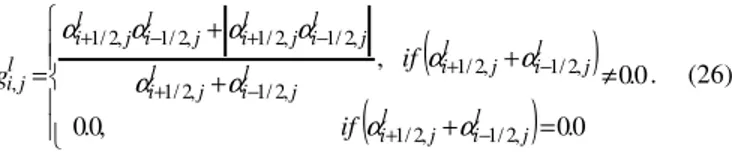
Figure 5. Pressure field (YK/85).
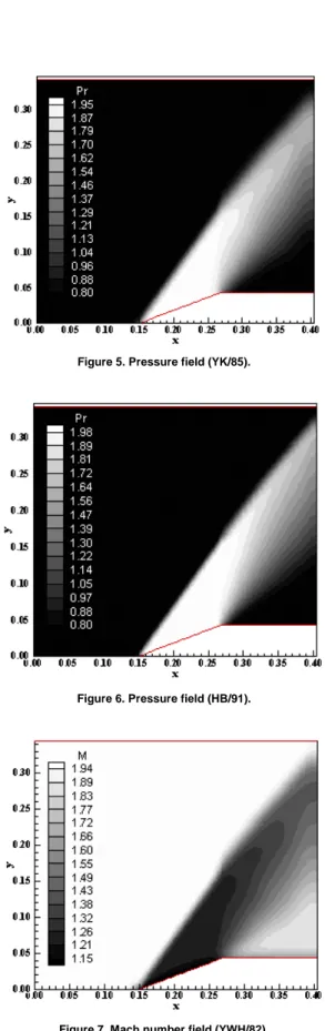
Figure 6. Pressure field (HB/91).
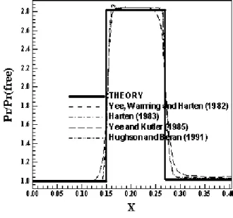
Figure 7. Mach number field (YWH/82).
(black area) than the Yee, Warming and Harten (1982) and the Yee and Kutler (1985) schemes.
Figure 8. Mach number field (H/83).
Figure 9. Mach number field (YK/85).
Figure 10. Mach number field (HB/91).
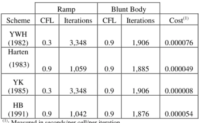
Figure 11 shows the wall pressure distributions along the ramp obtained by the Yee, Warming and Harten (1982), the Harten (1983), the Yee and Kutler (1985) and the Hughson and Beran (1991) schemes. They are compared with the oblique shock wave and the expansion wave Prandtl-Meyer theories. It is possible to note that the YWH/82 and the YK/85 solutions are smoother than
the H/83 and HB/91 solutions, but they do not present oscillations around the shock region, what characterizes better solutions, in qualitative terms, than the H/83 and HB/91. They are doing what high resolution schemes are expected to do: present solutions of second order schemes free of oscillations in shock regions. In the H/83 and HB/91 solutions, the shock presents a small peak, but the shock is thinner and the expansion fan is less smoothed. The HB/91 scheme is the only one which has the highest value of pressure exactly at the beginning of the ramp, where the shock position should be. The YWH/82 and the YK/85 schemes also present nearly the same solution in terms of pressure distribution.
Figure 11. Wall pressure distributions.
One way to quantitatively verify if the solutions generated by each scheme are satisfactory consists in determining the shock angle of the oblique shock wave, β, measured in relation to the initial direction of the flow field. Anderson (1984) (pages 352 and 353) presents a diagram with values of the shock angle, β, to oblique shock waves. The value of this angle is determined as function of the freestream Mach number and of the deflection angle of the flow after the shock wave, φ. To φ = 20º (ramp inclination angle) and to a freestream Mach number equals to 2.0, it is possible to obtain from this diagram a value to β equals to 53.0º. Using a transfer in Figures 3 to 6, it is possible to obtain the values of β to each scheme, as well the respective errors, shown in Tab. 1. The results highlight that the Hughson and Beran (1991) scheme is the most accurate of the studied schemes in this problem.
Table 1. Shock angle and percentage errors for the ramp problem.
Algorithm β (°) Error (%) Yee, Warming and Harten (1982) 54.2 2.26
Harten (1983) 53.9 1.70 Yee and Kutler (1985) 53.8 1.51 Hughson and Beran (1991) 53.2 0.38
Blunt Body Physical Problem
body mesh, respectively. The freestream Mach number adopted for this simulation as initial condition was 5.0, characterizing a high supersonic flow regime.
Figure 12. Blunt body configuration.
Figure 13. Blunt body mesh.
Figures 14 to 17 show the pressure field generated by the Yee, Warming and Harten (1982), the Harten (1983), the Yee and Kutler (1985) and the Hughson and Beran (1991) schemes, respectively. The pressure field generated by the H/83 scheme is the most intense in relation to the others schemes. Good symmetry properties are observed in all solutions.
Figure 14. Pressure field (YWH/82).
Figure 15. Pressure field (H/83).
Figure 16. Pressure field (YK/85).
Figure 17. Pressure field (HB/91).
Figure 18. Mach number field (YWH/82).
Figure 19. Mach number field (H/83).
Figure 20. Mach number field (YK/85).
Figure 22 shows the -Cp distribution around the blunt body geometry obtained by all four schemes. There are no meaningful differences among the solutions generated by the schemes, with all solutions obtaining the same value to the Cp peak at the configuration nose (Cp = 1.68).
Figure 21. Mach number field (HB/91).
Figure 22. -Cp distribution on the blunt body surface.
The aerodynamic coefficients of lift and drag are shown in Tab. 2 to each scheme. Due to the symmetry of the blunt body configuration in relation to the y axis and due to the zero angle of attack, the expected value to the lift coefficient (cL) is zero. As can be seen the best value is obtained by the Hughson and Beran (1991) scheme.
Table 2. Aerodynamic coefficients of lift and drag for the blunt body problem.
Algorithm cL cD
Yee, Warming and Harten (1982) 3.99x10⁻⁴ 4.82x10⁻¹ Harten (1983) 1.30x10⁻⁴ 4.82x10⁻¹ Yee and Kutler (1985) 3.99x10⁻⁴ 4.82x10⁻¹ Hughson and Beran (1991) 1.26x10⁻⁴ 4.81x10⁻¹
Another possibility for quantitative comparison of all schemes is the determination of the stagnation pressure on the configuration nose. In that region the shock wave presents a normal shock behavior and the stagnation pressure jump can be obtained from the tables encountered in Anderson (1984). With that it is possible to determine the ratio
pr
0pr
∞ , where pr0 is the stagnation pressure in front of the configuration and pr∞ is the freestream pressure (equal to 1/γ for the adopted nondimensionalization).pressure to each scheme and the respective percentage errors. As can be observed, the Harten (1983) scheme presents the most accurate value.
Table 3. Stagnation pressure for the blunt body problem.
Algorithm pr0 Error (%)
Yee, Warming and Harten (1982) 20.30 12.9 Harten (1983) 20.39 12.5 Yee and Kutler (1985) 20.30 12.9 Hughson and Beran (1991) 20.35 12.7
For the ramp and blunt body results, two schemes are the best in relation to the others. The solution generated by the Hughson and Beran (1991) scheme in the ramp problem, in the determination of the shock angle, is the most accurate, although the Yee, Warming and Harten (1982) and the Yee and Kutler (1985) schemes present better wall pressure distribution. In the blunt body problem, the solution generated by the Harten (1983) scheme is the most accurate with respect to shock jump conditions.
Table 4 presents the CFL number, the number of iterations to convergence and the computational cost of the algorithms in the present simulations. As can be seen, the Yee and Kutler (1985) scheme, the cheapest scheme, is about 810% less expensive than the Yee, Warming and Harten (1982) scheme, the most expensive.
Table 4. Numerical results from the simulations.
Ramp Blunt Body
Scheme CFL Iterations CFL Iterations Cost(1)
YWH
(1982) 0.3 3,348 0.9 1,906 0.000076 Harten
(1983) 0.9 1,059 0.9 1,885 0.000049
YK
(1985) 0.3 3,348 0.9 1,906 0.000008
HB
(1991) 0.9 1,042 0.9 1,876 0.000054 (1): Measured in seconds/per cell/per iteration
Conclusions
The present work compares the flux difference splitting TVD algorithms of Yee, Warming and Harten (1982), of Harten (1983), of Yee and Kutler (1985) and of Hughson and Beran (1991), all schemes second order accurate in space, applied to aeronautical and aerospace problems in the two-dimensional space. The Euler equations, on a finite volume context, using an upwind and a structured spatial discretization, were solved. A spatially variable time step was employed to accelerate the convergence process to the steady state solution. The steady state physical problems of the supersonic flows along a ramp and around a blunt body configuration were solved.
All schemes have presented good solutions in qualitative and quantitative terms. In the ramp problem, the Hughson and Beran (1991) scheme was the most critical because presented the most intense pressure field and Mach number field in relation to the other schemes. The shock and the expansion fan are better captured by the Yee, Warming and Harten (1982) and the Yee and Kutler (1985) schemes, even though they are smoother than the solutions
generated by the Harten (1983) and the Hughson and Beran (1991) schemes, which presented a shock peak. The shock angle is best estimated by the Hughson and Beran (1991) scheme. In the blunt body problem, the Harten (1983) scheme presented the most intense pressure field in relation to the other schemes, characterizing the most critical solution. The Mach number and the pressure coefficient distributions of all schemes were practically the same. The lift aerodynamic coefficient was better predicted by the Hughson and Beran (1991) scheme. The stagnation pressure on the configuration nose is best determined by the Harten (1983) scheme. The Yee and Kutler (1985) scheme, the cheapest scheme, is about 810% less expensive than the Yee, Warming and Harten (1982) scheme, the most expensive. The Yee, Warming and Harten (1982) and the Yee and Kutler (1985) schemes have presented virtually the same solutions, where the different forms of defining the artificial compressibility terms of both schemes do not present meaningful differences. A more complete study, with more physical problems, will be carried out by this author aiming to better highlight the characteristics of these schemes.
As initial conclusion, the Harten (1983) and the Hughson and Beran (1991) TVD schemes are better than the Yee, Warming and Harten (1982) and the Yee and Kutler (1985) TVD schemes. References
Anderson, J. D., 1984, “Fundamentals of Aerodynamics”, McGraw-Hill, Inc., EUA, 563p.
Harten, A., 1983, “High resolution schemes for hyperbolic conservation laws”, Journal of Computational Physics, Vol. 49, pp. 357-393.
Hughson, M. C., and Beran, P. S., 1991, “Analysis of hyperbolic blunt-body flows using a total variation diminishing (TVD) scheme and the MacCormack scheme”, AIAA 91-3206-CP.
MacCormack, R. W., 1969, “The effect of viscosity in hypervelocity impact cratering”, AIAA Paper 69-354.
Maciel, E. S. G., 2002, “Simulação Numérica de Escoamentos Supersônicos e Hipersônicos Utilizando Técnicas de Dinâmica dos Fluidos Computacional” (in Portuguese), Ph.D. thesis, ITA, CTA, São José dos Campos, SP, Brazil, 258 p.
Maciel, E. S. G., 2005, “Analysis of convergence acceleration techniques used in unstructured algorithms in the solution of aeronautical problems – part I”, Proceedings of the 18th COBEM International Congress of Mechanical Engineering, Ouro Preto, MG, Brazil.
Maciel, E. S. G., 2006, “Comparison between the Yee, Warming and Harten and the Hughson and Beran high resolution algorithms in the solution of the Euler equations in two-dimensions – theory”, Proceedings of the 27th CILAMCE Iberian Latin-American Congress on Computational Methods in Engineering, Belém, PA, Brazil.
Maciel, E. S. G., 2007a, “Comparison among structured first order algorithms in the solution of the Euler equations in two-dimensions”,
Journal of the Brazilian Society of Mechanical Sciences and Engineering, Brazil, Vol. 29, No. 4, pp. 420-430.
Maciel, E. S. G., 2007b, “Comparison among predictor-corrector, symmetrical and TVD upwind schemes in the solution of the Euler equations in two-dimensions – theory”, Proceedings of the 19th COBEM International Congress of Mechanical Engineering, Brasília, DF, Brazil.
Roe, P. L., 1981, “Approximate Riemann solvers, parameter vectors, and difference schemes”, Journal of Computational Physics, Vol. 43, pp. 357-372.
Yee, H. C., and Kutler, P., 1985, “Application of second-order-accurate total variation diminishing (TVD) schemes to the Euler equations in general geometries”, NASA-TM-85845.