! " # # $ %
&
' ( ) *
! " # # $ %
!
A variational formulation and solution of general three-dimensional potential flows gave rise to the construction of a special family of ‘trial functions’. This family is composed by circular-sector vortex rings, here named
α
-rings, i.e., rings that are positioned on the border of a circular sector with aperture angleα
. An explicit formula for the velocity potential describing theα
-rings family is here derived. A particular case is the well-known circular vortex-ring. The formula is given in terms of a uniformly valid series involving trigonometric and Hypergeometric functions. Results concerning the complete circular ring are compared to the well-known solution given, in closed form, in terms of Bessel functions, validating the present formula. Convergence is discussed. Graphical examples are shown for various rings of different sector angles. As an elementary application, the steady potential flow around three-dimensional bodies in unbounded fluid is formulated and solved under the variational approach. The variational method is fully validated through the sphere problem and for a family of spheroids. Examples concerning either translatory or rotatory motion around a transversal axis are presented for the spheroid family.Keywords: potential flow, sector vortex-rings, variational method, three-dimensional bodies
Introduction1
23Potential flow problems around three-dimensional bodies
represent a core of important applications in hydrodynamics. Particularly the hydromechanic interactions of floating bodies with free-surface waves, usually referred to as the radiation and diffraction problems, form a formidable source of very interesting and practical applications in marine hydrodynamics and ocean engineering.
A number of methods, as those based on the Green function method, are well established in this area, leading not only to the solution of linear (first-order) problems but also to the high-order ones. Nevertheless, the precise computation of some important hydrodynamic coefficients, as added mass or wave-damping terms, depends on the degree of accuracy obtained in the solution of the respective potential problem, particularly in regions where the curvature of the body surface is high, as in the neighborhood of sharp edges. A high degree of mesh refinement is usually applied locally, leading then to intensive numerical work.
On the other hand, variational approaches are rather common in continuum mechanics and, despite being classical, have been subject of many and recent investigations; see, e.g., Irshik & Holl, 2002, Mušicki, 2005. A previous, general and rigorous treatment of such a matter can be found in Seliger & Whitham, 1968. Such approaches are quite powerful, enabling to treat dynamical problems in a systematic and rather general way. In this context, the application of Lagrangian formalisms to problems involving the interaction of bodies with a liquid flow - sometimes named hydromechanics, whenever the kinetic energy of the fluid is given in terms of the
Paper accepted January, 2008. Technical Editor: Francisco Ricardo Cunha.
2
This article is an updated extract of an unpublished monograph, written by the authors in 1998, under the same title.
well-known added mass tensor - is also classic; Lamb, 1932, art. 137.
In the above cited linear radiation and diffraction problems, a variational approach was successfully used, for instance, leading to a variational method; see Aranha & Pesce, 1989. In this method all the hydrodynamic coefficients are shown to be stationary points of well-defined functionals, analogous to the well-known Rayleigh quotient in applied mechanics. The most important consequence of this fact is that a considerably rough approximation for the potential solution, with error of orderδ, say, gives rise to an order δ2-error approximation for the hydrodynamic coefficients. The variational solution is searched in a finite-dimensional space, spanned by a set of conveniently chosen ‘trial functions’. Elementary singularities can be elected to form the core of such a set, like poles, dipoles, line densities of poles and dipoles. The set of ‘trial-functions’ must satisfy the field equation (Laplace) and some of the boundary conditions (or, likewise, conditions at infinity), but the corresponding natural condition on the body surface. This latter condition is enforced by solving the variational ‘weak equation’ that arises from the variational formulation.
Systems composed by rectilinear line vortices were used, together with poles, dipoles and related elementary solutions, as ‘trial functions’, efficiently completing the construction of a finite-dimensional space in which the solution of three-finite-dimensional potential flows around advancing bodies was determined with accuracy; Pesce et al, 1997. A special family may be also sought, however, that not only comprises much of the behavior of dipoles, but does have the additional and important ability of representing the large variations in the potential solution in the neighborhood of high curvature regions: a family of vortex rings or reentrant vortex filaments. Even more complex problems, as the radiation and diffraction of water waves by floating bodies, might make use of this ability.
of the well-known circular line vortex potential in unbounded fluid, into a useful family, is not so trivial. We should remember that even the simple circular vortex ring potential is given in terms of elliptic integrals (see Lamb, art. 161), or can be constructed in terms of hypergeometric functions and Legendre polynomials (Lamb, art.84) or else, in terms of Bessel functions (Lamb, art. 161 and 102).
The formula here presented for the α-rings family is given in terms of a uniformly valid series involving simple trigonometric functions and hypergeometric functions or, alternatively to the latter, in terms of incomplete Beta functions. The results have been tested concerning convergence, and by properly stating analytic continuations and asymptotic behaviors. Results have been fully and consistently compared to the circular vortex solution. Examples concerning some particular α-angle values are shown in detail.
The α−rings family is then used within the variational method. Firstly the sphere problem is addressed, validating the method and the vortex family: the analytical solution is completely recovered with the use of only one vortex ring. Then, a family of oblate spheroids is analyzed, for which the analytical solution is also available, in either steady translatory or rotatory motion around any transversal axis, when the α−rings family demonstrates its ability.
Nomenclature
a = sphere radius, or semi-diameter of revolution of an oblate spheroid, or a parameter
jj
a = nondimensional added mass tensor
) , , (z pq
B = the incomplete Beta function b = radius of an oblate spheroid, or a parameter c = parameter
) ; ; ; (abcw
F = Hypergeometric function )
, (φψ kl
F = Rayleigh quotient functional )
, (φψ
G = kinetic energy functional
[
G(Ti,Tj)]
=G = kinetic energy matrix )
, (ϕα n
I = recursive trigonometric function
) (
Lφ = Lagrangian of the potential field φ kl
m = added mass tensor
kl
m~ = variational approximation for the added mass tensor n = natural number
q = vector of coefficients R = radius of the vortex ring r = distance
r = position vector ) , ( 2 1
φ φ ρG
T= = kinetic energy of the potential field φ
) (r j
T = trial function
U = free stram velocity vector )
(ψ
V = work functional
{
V(Ti)}
=
V = work vector )
; , , (ξ ζ ϕ α
ξ
v = nondimensional velocity ξ−component )
; , , (ξ ζ ϕα
ζ
v = nondimensional velocity ζ−component )
; , , (ξ ζ ϕ α
ϕ
v = nondimensional velocity ϕ−component )
V (
) 1 ( 2
W = Sobolev space
z = height in cylindrical coordinates
Greek Symbols
α = aperture angle of a circular sector of radius R δ = variation
r U⋅ + =
Φ φ = velocity potential function φ = velocity potential function
) ( ~
r
φ = variational approximation for φ
Γ = Gamma function. κ = strength of a vortex filament
ρ = radial variable in cylindrical coordinates θ = angular variable in cylindrical coordinates
) (r
ψ = square integrable function ξ = nondimensional ρ
ζ = nondimensional z
ΩP = solid angle subtended at P by any diaphragm that closes the ring C
Mathematical Formulation
The theoretical basis for the study of vortex rings or reentrant vortex filaments, (or even else, closed line vortices) was well established since the end of the nineteenth century. Lamb dedicates an entire chapter (VII) to the study of vortex motion, giving some emphasis to the analysis of vortex rings. Truesdell, 1954, in his thorough Kinematics of Vorticity puts some attention on the subject, but only from the conceptual perspective. Saffman, 1992 in his superb and complete monograph on vortex dynamics, treats the problem in depth, but attributes minor practical importance to its use when, concerning the singular behavior of the Bio-Savat integral as distance r to the line goes to zero, states that (page 37) “the logarithmically infinite, non-circulatory, velocity along the binormal inhibits the curved line vortex (of zero-cross-section) from being a useful dynamical model”.
Nevertheless, if kinematics of potential flow around three-dimensional bodies is concerned, vortex rings can play an important practical role. In fact, as well known, perturbed potential flows resulting from the presence of a body, behave asymptotically like dipoles and, as pointed out by Saffman, “the line vortex is kinematically equivalent to a surface distribution of dipoles with uniform density, the axis of the dipoles being aligned along the normal to the barrier ”.
It is not difficult to visualize the superposition of a circular vortex and a uniform stream: a spheroidal-like body. In fact the curious Hill spherical vortex (see Lamb, art. 165) gives the exact solution for the flow pasting a sphere. Moreover, a line vortex might help, as emphasized before, to simulate the very large variation in the velocity field near regions of high curvature, as the edges of a finite cylinder advancing along its own axis or even rotating around any transversal axis.
Vortex Rings
As shown for instance in Milne-Thomson, 1979, page 572, if the vorticity is concentrated into a single closed vortex filament C, being κ the strength, i.e. ‘the product of the magnitude of the vorticity and the (infinitesimal) area of the cross-section of such a filament’, the potential velocity induced at a point P is given by
dS r n S
=
∫∫
14 ∂
∂ π κ
φ (1)
P S
dS
r = Ω
= κπ
∫∫
θ κπφ
4 cos
4 2 (2)
where ΩP is the solid angle subtended at P by any diaphragm that closes the ring C. The velocity potential φ is a many-valued function decreasing or increasing by 4π as P rounds the filament once. However, as pointed out by Saffman, 1992, page 35, “it can be made single valued by introducing a barrier consisting of a surface bounded by the vortex, across which the velocity potential jumps by amount of -κ”.
Circular Vortex Rings
Let the vortex filament be of circular form. In this important particular case the potential can be either expressed by means of complete elliptic integrals, as in the analogue case concerning electro-magnetic phenomena; Jackson, 1975, section 5.5, or in a more tractable manner, expressed in closed form involving Bessel functions. In fact, see Lamb, Art. 161 and 102, taking polar cylindrical coordinates, with z as the symmetry axis, the velocity potential of a circular vortex ring, of radius R, positioned at the plane z=0, can be proven to be given by,
∫
∞ − =
0
1
0( ) ( )
2 1 ) ( sign ) ; ,
(ρ z R z κR e kzJ kρ J kRdk
φ (3)
The corresponding stream function reads, for z > 0
∫
∞ − −
=
0
1
1( ) ( )
2 1 ) ; ,
(ρ z R κRρ e kzJ kρ J kR dk
ψ (4)
As pointed out by Lamb, the regions inside and outside the circle constitute two distinct equipotential surfaces (a jump occurs) over which it was assumed
κ ρ
φ ρ φ
2 1 ) ; 0 , (
0 ) ; 0 , (
± = <
= >
± R
R R R
(5)
Well known, besides remarkable, is the already mentioned fact that the value of φ is the same as that corresponding to a system of dipoles distributed over the whole circle with a constant density κ. As it will be seen, this behavior is one of the reasons for the good performance achieved when vortex rings are chosen as elementary trial functions spanning a proper vector space in which a solution for the flow around a body is searched, by means of a variational method. Moreover and intuitive, vortex rings may be suitable representations for the local potential flow around sharp edges, as in the case of a moving cylinder along its own axis of symmetry.
Circular-Sector Vortex-Rings or αααα-Rings
Let now the vortex filament be placed over the border of a circular sector of radius R and aperture angle α as shown in Figure 1. This kind of rings will be named “αααα-rings”. The circular vortex ring is, of course, a particular case when α=2π : a ‘2π-ring’.
Take then, as shown in Figure 1, a α-ring with radius R, aperture angle α, at the plane z=0.
ϕ
P
ρ
α
0 O
z
R
κ
Figure 1. Circular-sector vortex ring or ‘αααα-ring’
Let the circular sector be the surface S in Eq.(3), P’ being a point of integration, inside the diaphragm enclosed by the ring, and P a point at which the velocity potential is searched for. Elementary geometry gives Eq.(2) in polar cylindrical coordinates in the form
(
ρ ρ ϕ ϕ)
ϕ ρρ
π κ α ϕ ρ φ
α
′ ′ −
′ − + ′ + ′ =
=
∫
∫
d dz I
zI R
z
R
0
2 3 2
2 2
0 2cos( )
1 4 ) , ; , , (
(6)
By a convenient transformation in the integrand the velocity potential function can be expressed in terms of incomplete elliptic integrals of second kind for a general angle α. This derivation will not be worked out here, however; see Batchelor, chapter 7, section 7.2 for similar reasoning applied to the stream function of a complete vortex ring. This solution is not explicit but still given in closed form.
Perhaps a wiser manner, or at least an alternative form, to deal with the problem is to separate the angular dependence by transforming and then expanding the integrand in a standard power series. For, let
2 3 2 2 2
2 2 2
) (
) ; , (
2 ) ; , (
− + ′ + = ′
+ ′ +
′ =
′
z z
z z
ρ ρ ρ ρ η
ρ ρ
ρ ρ ρ
ρ γ
(7)
By applying the above defined functions Eq.(6) transforms into
(
γ ρ ρ ϕ ϕ)
ϕ ρρ ρ η ρ
π κ α ϕ ρ φ
α
′ ′ −
′ ′ −
′ ′
=
=
∫
∫
d dz z
I
zI R
z
R
0
2 3 0
1
1
) cos( ) ; , ( 1
1 )
; , (
4 ) , ; , , (
(8)
Notice that
1 2 ) (
2 2
2 2
2 − ′ + ′≤
′ =
′ +
′ ≤
ρ ρ ρ ρ
ρ ρ ρ
ρ ρ ρ
γ , so
1 ) cos(ϕ′−ϕ ≤
γ (9)
1 ; ! 2 )! 1 2 ( 1 ) 1 ( 1
1 2 2
2 3 < + + = −
∑
∞= ε ε
ε n n n n n (10)
Eq.(8) can be written in the following form,
ϕ ϕ ϕ ρ ρ γ ρ α ρ ρ η ρ π κ α ϕ ρ φ α ′ − ′ ′ = ′ + + ′ ′ =
∫
∫
∑
∞ = d z G d G n n z z R z n n R n n 00 1 2 2
) ( cos ) ; , ( ) ! 2 )! 1 2 ( )( ; , ( 4 ) , ; , , ( (11)
Defining the integrals
[
]
) , ( 1 sin cos ) sin( ) ( cos 1 ) , ( sin ) sin( ) , ( ) , ( ) ( cos ) ; ( 2 1 1 1 0 0 α ϕ ϕ ϕ ϕ α ϕ α α ϕ ϕ ϕ α α ϕ α α ϕ ϕ ϕ ϕ α ϕ α − − − − + + + − − = + − = = ′ − ′ =∫
n n n n n n I n n n I I I d I (12)where the recursive relationship immediately comes from elementary calculus, Eq.(11) can be put in the form
) ; , ( ) ; ( ! 2 )! 1 2 ( 4 ) , ; , , ( 0 2 R z g I n n R z R
z n n
n n ρ α ϕ π κ α ϕ ρ
φ
∑
∞= + = (13) being
(
)
2 2 2 2 10 2 2 32
1 0 ) ; , ( where , = ) ( ) ; , ( ) ; , ( or , ) ; , ( ) ; , ( 2 ) ; , ( R z R z du u u f R z r f R R z g d z z R R z g n n n n n n R n n n + = + = ′ ′ ′ ′ =
∫
∫
+ + ρ ρ σ σ σ ρ ρ ρ ρ ρ ρ η ρ ρ γ ρ (14)It follows at once that, for n=0,
) 1 1 ( 1 ) ( ) ; , ( 2 0 0 σ σ σ σ ρ + − = = f R z f (15)
For n≥1, however, the definite integral in equation (14) can be written in terms of Hypergeometric functions (see Appendix A) leading to 1 ) ; 2 2 ; 2 3 , 2 1 ( ) ( 1 ) 2 ( 1 ) ( ) ; , ( 2 2 3 2 > − + + + × × + = = − + σ σ σ σ ρ n n n F n f R z f n n n (16)
The Hypergeometric functionF(a;b;c;w);w∈C is usually expressed in terms of the Gauss Hypergeometric series, see
Abramowitz & Stegun, 15.1.1, or Erdélyi, Magnus, Oberhettinger and Tricomi, 1953, v.1, chapter II, as
∑
∞= =
0 ( ) !
) ( ) ( ) ; ; ; ( k k k k k k w c b a w c b a F (17), Where 1,2,3... = ); 1 ( ) 1 ( ) ( ) ( ) ( 1 ) ( 0 k k a a a a k a a a
k = + ⋅ ⋅⋅ + −
Γ + Γ = = (18a) or, explicitly, + + + + + + + + + = ;... ) 2 )( 1 ( ) 2 )( 1 ( ) 2 )( 1 ( ; ) 1 ( ) 1 ( ) 1 ( ; . ; 1 ) ( ) ( ) ( c c c b b b a a a c c b b a a c b a c b a k k k (18b)
The Gauss series is convergent in the circle w<1. In equation (16) this condition holds if σ2 >1, i.e.,
1 2 2 2 > + R z ρ (19)
i.e., outside the sphere of radius R (the sphere of non-dimensional radius 1). However, constructing the analytic continuation of (16) (Appendix B; see Erdélyi, Magnus, Oberhettinger & Tricomi, 1953, pp. 105-108) we get a uniformly valid formula, for all σ >0,
) ) 1 ( 1 ; 2 2 ; 2 2 1 , 2 1 ( ) 1 ( ) ) 1 ( 1 ; 2 2 ; 1 , 2 3 ( ) 1 ( ) ; 2 2 ; 2 3 , 2 1 ( 2 2 2 σ σ σ + + − + − = + + + − = − + + + − − − n n n F z n n F z n n n F a b
so that Eq.(16) can be replaced by
0 all ) ) 1 ( 1 ; 2 2 ; 1 , 2 3 ( ) ( 1 ) 2 ( 1 ) ( ) ; , ( 2 2 3 2 > + + + + = = = + σ σ σ σ ρ n n F n f R z f n n n (16a)
or, alternatively, by
0 all ) ) 1 ( 1 ; 2 2 ; 2 2 1 , 2 1 ( ) ( 1 ) 2 ( 1 ) ( ) ; , ( 2 2 2 3 2 > + + − + × × + = = + σ σ σ σ ρ n n n F n f R z f n n n (16b)
The final formula for the velocity potential function is then given by
n
n n
n n R
R z f I n n R z R z + =
∑
∞ = ρ ρ α ϕ π κ α ϕ ρφ ( ; ) ( , ; )
! 2 )! 1 2 ( 4 ) , ; , , ( 0 2 (20)
n n n
n n
f I n
n ϕα σ ξ
ζ π α ϕ ζ ξ
φ ( ; ) ( )
! 2
)! 1 2 ( 4
1 ) ; , , (
0 2
∑
∞=
+
= (20a)
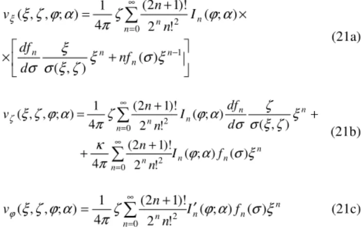
The usefulness of the Hypergeometric functions, despite some technical difficulties concerning the above-mentioned series, resides in the recursive relationships involving the derivatives, as those will be necessary in computing the velocity field. In polar cylindrical coordinates, the velocity components, in nondimensional form read (see Appendix C),
+ ×
× +
=
− ∞
=
∑
1
0 2
) ( )
, (
) ; ( ! 2
)! 1 2 ( 4
1 ) ; , , (
n n n n
n
n n
nf d
df
I n n v
ξ σ ξ
ζ ξ σ ξ σ
α ϕ ζ
π α ϕ ζ ξ
ξ
(21a)
n n n
n n
n n
n
n n
f I n n
d df I
n n v
ξ σ α ϕ π
κ
ξ ζ ξ
σ ζ
σ α ϕ ζ
π α ϕ ζ ξ ζ
) ( ) ; ( ! 2
)! 1 2 ( 4
) , ( ) ; ( ! 2
)! 1 2 ( 4
1 ) ; , , (
0 2
0 2
∑
∑
∞
= ∞
=
+ +
+ +
=
(21b)
n n n
n n
f I n n
v ζ ϕ α σ ξ
π α ϕ ζ ξ
ϕ ( ; ) ( )
! 2
)! 1 2 ( 4
1 ) ; , , (
0 2
′ +
=
∑
∞=
(21c)
Notice that the Gauss series in Eq.(16a) (and (C11a)) are not convergent if σ =0. However the asymptotic limit for the potential function for ξ=0 is given, in non-dimensional form, by (see Appendix C)
+ − =
2
1 1 4 ) ; , 0 (
ζ ζ π
α ζ ζ α ζ
φ (22)
so that,
π α α φ
4 ) ; 0 , 0
( ± =± (23)
Notice (see Appendix C) that the asymptotic behavior as
∞ →
σ is, in nondimensional form,
∞ →
≈ σ
σ ζ π α α ϕ ζ ξ
φ ;
2 4 ) ; , , (
3 (24)
so that
ξ ζ
ζ π α α ϕ ζ ξ
φ ; , allfinite
2 1 4 ) ; , , (
2 →±∞
±
≈ (25)
In words, the vortex ring behaves like a ζ-dipole, as expected, what completes the analysis. It should be noticed that analogous formula for the velocity potential could be obtained by the classical expansion of the potential function in spherical harmonics; see Lamb, arts. 84-86.
Circular Vortex Ring
A particular case is the ‘complete’ circular vortex ring (α =2π). The integrals in Eq.(12) are now simplified into,
) 2 , ( 1 ) 2 , (
0 ) 2 , (
2 ) 2 , (
2 1
0
π ϕ π
ϕ π ϕ
π π ϕ
−
− = = =
n
n I
n n I
I I
(26)
and, obviously,
0 ) 2 ,
( =
′ ϕ π
n
I (27)
Equations (20a) (and (C13a,b)), with (C27), (C28), will be used for numerical comparison purposes with the closed-form solution given by Eq.(3).
Numerical Analysis and Examples
This section is dedicated to the numerical validation of the present formulation as well as to discuss interesting features of this particular kind of potential flow, through some selected examples. Convergence is not exhaustively discussed but only exemplified by means of numerical experiments.
Numerical Examples for a ‘Complete’ Vortex Ring
We start by comparing, for the complete vortex ring, the present formulation (Equations 20a-26, 27) with the closed form solution given by Eq.(3). The vortex ring of unit radius is circular, positioned at plane z=0.
Figures 2 and 3 show, as function of radial distance, the comparison between the present formulation and the closed form solution Eq.(3) for the velocity potential function. Two distinct values of z, corresponding to ζ =0.5;1.0 are taken. N is the number of terms in the truncated series. The agreement is complete in the whole range.
Figure 4a,b shows the same comparison, but now as a function of axial distance z, for radial distance, ξ=ρ/R=0.5 and for N=30,200. The agreement is very good for ζ=z/R>0.3, but convergence rate is slow for smaller values. Notice that the jump in the potential caused by the presence of the potential barrier is noticeable but can be better represented by the present formulation if the number of terms in the series is increased. If N is increased further, graphical results become undistinguishable. The asymptotic representation for the unitary jump provided by the series is quite evident. In fact, Figures 5a,b show this behavior quite well, for ξ=ρ/R=1.0.
Figures 6a,b show the axial component of velocity for two different values of z. Notice that there is a value for ζ=z/R below which the maximum absolute value is no more in the center, but at a distance ξ=ρ/R that goes to 1 as ζ→0. In Fig.7a the curve below represents the solution given by Eq.(3). In Fig.7b curves corresponding to the present solution and to equation (3) are undistinguishable. Series are truncated at N=100, even though N=30 would be enough for the curves corresponding to ζ >0.5.
ξξξξξξξξ
ξξξξξξξξ
Figure 3. Nondimensional Velocity Potential for a ‘Complete’ Circular Vortex Ring comparison between present formulation (♦♦♦♦) and closed form solution (3); α====2π;ζ====zR====1.0;N====30.
(a) α=2π;ξ=ρ R=0.5;N=200
(b) α=2π;ξ=ρ R=0.5;N=200
Figure 4. Nondimensional Velocity Potential for a ‘Complete’ Circular Vortex Ring comparison between present formulation (♦♦♦♦) and closed form solution (4).
(a) α=2π;ξ=ρ R=1.0;N=30
(b)α=2π;ξ=ρ R=1.0;N=150
Figure 5. Nondimensional Velocity Potential for a ‘Complete’ Circular Vortex Ring comparison between present formulation (♦♦♦♦) and closed form solution (3).
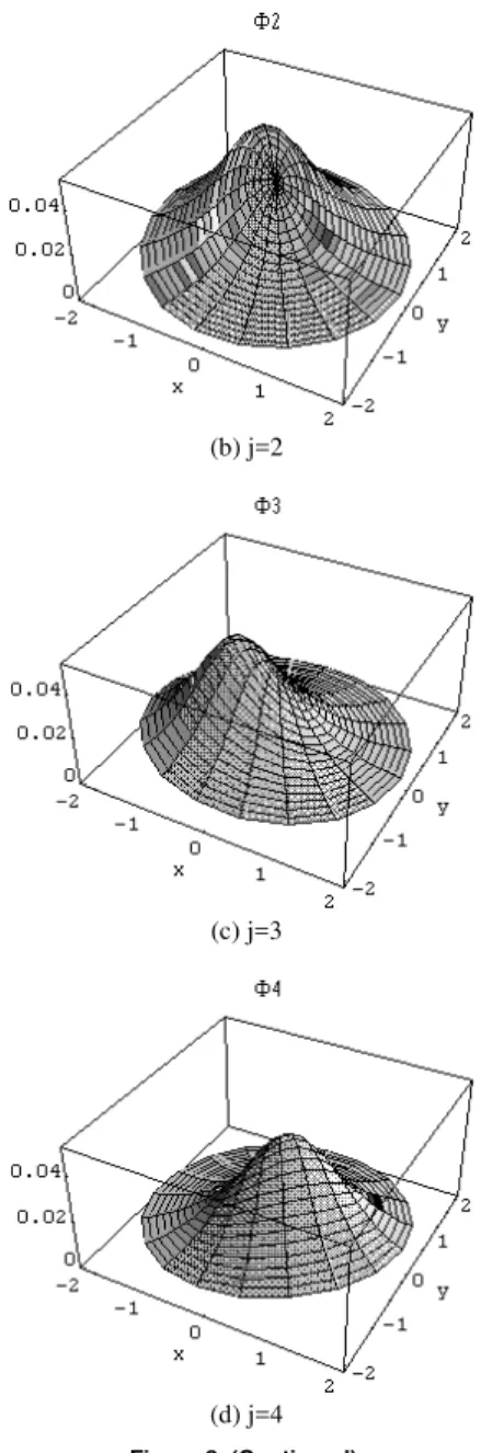
As 3D-plot examples, Figures 7a,b,c,d show the potential function and the three velocity components for a quarter- vortex rings α=π/2. Notice that for ζ=1.0 convergence is verified for N=30. Notice also the presence of the azimuthal component.
Finally, a complete circular vortex ring was taken again as the paradigm, in order to confirm the numerical results for arbitrary α. In fact we can construct the complete circular vortex ring with a sequence of 2π/K-rings, in the form
∑
=
− − = K
j K K
j 1
2 ; 2 ) 1 ( , , ) 2 ; , ,
(ξ ζ ϕ π φ ξζ ϕ π π
φ (28)
Figure 8 shows such a construction for the case treated above,α=π/2 (Κ=4). Notice that the agreement is complete, comparison with the paradigm being undistinguishable.
ξξξξξξξξ
(a) ζ =z R=0.25
ξξξξξξξξ
(b) ζ=z R=1.00
Figure 6. Nondimensional Axial Velocity Component for a ‘Complete’ Circular Vortex Ring; comparison between present formulation (♦♦♦♦) and closed form solution (3);α====2π;ζ====zR====0.25;1.0;N====100.
(a) potential function
Figure 7. Nondimensional Potential and Cylindrical Polar Velocity
Components for a ‘Quarter’ Circular Vortex Ring;
30 0 1 2 ==== ==== ====
====π ;ζ zR .;N
vξξξξ vξξξξ
(b) radial velocity component
vζζζζ vζζζζ
(c) axial velocity component
vφφφφ vφφφφ
(d) azimuthal velocity component
Figure 8. (Continued).
(a) j=1
Figure 8. Nondimensional Potential for a system of 4 ‘Quarter’ Circular Vortex Ring. α====π2;ζ====zR====1.0;N====30.
(b) j=2
(c) j=3
(d) j=4
Figure 8. (Continued).
ξξξξξξξξ
Figure 8(e). Constructed circular vortex-ring with 4 ‘quarter-rings (♦♦♦♦)’.
Comparison with a closed form solution, eq. (3).
30 0 1 2 ==== ==== ==== ====π ;ζ zR .;N
α .
A Variational Application to Potential Flows Around Bluff Bodies in Unbounded Liquid
variational method is to adopt a “dessingularized” approach. Numerical problems with singularities are avoided since the trial functions are placed “inside” the body. No singularities therefore exist concerning integrations over the body surface.
The Variational Approach
Consider a standard problem concerning a stationary incompressible and irrotational flow around a body described by a velocity potential,Φ, satisfying the usual field equation and boundary conditions
∞ → → Φ ∇
= ⋅ Φ ∇
= Φ ∇
r U n
,
on 0 0
2
S (29)
being S the body surface and n the unit outward (from the fluid body) normal vector. We write
r U⋅ + =
Φ φ (30),
where φ(r) is the perturbed velocity potential, due to the presence of the body in the otherwise steady stream, with constant velocity
U, satisfying
) r 1 (as
on -0
3 2
∞ → → ∇
= ⋅ − = ⋅ ∇
= ∇
r 0,
n U n
φ φ φ
S
Un (31).
Let ψ(r) be any square integrable function in the sense of the energy norm
( )
[
]
12V 2
V d
∫
∇= ψ
ψ (32)
This class of functions is a Hilbert space (W2(1)(V) in the specialized literature). Defining now the functional
) V ( ,
; V )
,
( 2(1)
V d W
Gφψ =
∫
∇φ⋅∇ψ φψ∈ (33)the kinetic energy associated to the perturbed potential can be written4
) , ( 2 1
φ φ ρG
T= (34)
Taking now the Laplacian of φ Eq.(31a), multiplying it by
ψ
, integrating in the whole infinite fluid volume and using the divergence theorem together with the boundary conditions given by Eq.(33b,c) we get an weak equation for the potential problem) V ( all
; ) ( ) ,
( V W2(1)
Gφψ = ψ ψ∈ (35)
Where
∫
∫
− =
⋅ ∇ =
S n
S dS U V
dS G
ψ ψ
ψ φ ψ φ
) (
) ,
( n
(36).
4
The same symbol ρ is here used for mass density, as usual.
Notice that the Lagrangian of the fluid system can be put in the form
) ( ) , ( 2 1 ) (
Lφ = ρGφ φ −ρV φ (37)
and, as we treat a stationary problem, that the Lagrange equation comes from the stationarity condition for L(φ), namely
0 ) ( Lφ =
δ (38).
It is a standard exercise on variational calculus to prove that (38) just imply the weak equation (35) and reciprocally.
Let now a numerical approximation for φ(r) be denoted by )
( ~
r
φ . The weak equation (37) will be solved in a finite dimensional sub-space of finite energy spanned by a linearly independent set of ‘trial functions’
{
Tj(r);j=1,...,N}
. The ‘trial functions’ are chosen to satisfy Eq.(31a) and Eq.(31c). We write∑
=
= N
j j jT q
1
) ( )
( ~
r r
φ (39)
that transforms Eq.(35) into a linear algebraic system in the unknown coefficients
{
qj;j=1,...,N}
[
]
{ }
{
V(T)}
q ) T , T ( G
i j
j i
= =
= =
V q G
V Gq with
(40).
It should be noticed that solving Eq.(40) is, in fact, to search for a stationary point of the Lagrangian (a minimum in this case), the result so obtained being the best approximation in the finite sub-space spanned by
{
Tj(r);j=1,...,N}
.Notice also that, considering the solution φk(r′); k=1,2,...,6 for a unitary velocity or rotation in the direction of xk, now in the body reference frame, such that
) 1 (as
6 , 5 , 4 ; ) (
3 , 2 , 1 ; on and , 0
3 3
2
r k v
k n v
S v
k k k
k k k
k k
k
∞ → → ∇
= ×
′ =
= = ⋅ =
= ⋅ ∇
= ∇
− r 0,
n r
n u
n
φ φ φ
(41)
the added mass tensor can be written in terms of the defined functionals as
) ( ) ( ) , ( ) ,
( k l l k k l l k
kl G G V V
m ρ= φ φ = φ φ = φ = φ (42)
With
∫
= S k
k v dS
V (ψ) ψ (43)
and where the usual reciprocity (symmetry) relations were shown explicitly.
As in Aranha & Pesce (1989), let
) , (
) ( ) ( ) , (
ψ φ
ψ φ ψ φ
G V V
be a functional defined in the Cartesian product space (V)
(V) 2(1)
) 1 (
2 W
W × 5. Then
) , ( k l kl kl F
m =ρ φ φ (45)
If we write for the finite-space solution
) ~ ( ) ~ ( ) ~ , ~ ( ) ~ , ~ ( ~
k l l k k l l k
kl G G V V
m
φ φ φ
φ φ φ
ρ = = = = (46)
Where
6 ,..., 1 ; ~
= +
= k k k
k φ δφ
φ (47)
it can be shown (see Appendix D) that ψ
ψ
δφ ,~) 0; all~
( k =
G (48)
or, in words, that a Galerkin orthogonality condition holds, as pointed out above. This leads to
) , ( ~
l k kl
kl m G
m = +ρ δφ δφ (49)
finally yielding (see Aranha & Pesce, 1989, for mathematical details)
{
}
[
]
2;
max k l
kl c
m δφ δφ
δ ≤ (50)
where c is an independent constant.
Notice that in terms of the ‘trial-functions expansion’ the added mass tensor is written
∑ ∑
= =
= N
i N j
l j k i l j k i
kl q qGT T
m
1 1
) , (
~ ρ (46a)
The results (equations 48-50) indicate that the variational method provides an approximation for the added mass tensor coefficients with an error of order δ2, if δ is the error of the
approximated potential solution.
Notice also that from Eq.(32) and Eq.(48), see Appendix D,
[
]
12[
]
12[
]
12) ( )
, ( ) ,
( k k k k k k
k Gδφ δφ Gφ δφ V δφ
δφ = = = (51)
As a matter of fact this method is rather general and can be extended and applied for problems satisfying more complex boundary conditions (see Aranha & Pesce, 1989), as in the case of a multi (rigid) body system, even in the presence of a free surface (see Pesce, 1988) or, e.g., for flexible bodies with the b.c.’s corresponding to each vibration mode.
The choice of the ‘trial function’ set is particular for each problem. In the present case, stationary and incompressible potential flow around bodies in unbounded fluid, an interesting choice could comprise poles, dipoles, line and surface densities of poles and dipoles and, of course and of our present interest, vortex rings. Previous work on the variational method (Aranha and Pesce, 1989) has shown that a proper choice of the trial functions, based on the expected flow pattern, may reduce drastically the number of trial functions required for convergence. Anyway, this is not mandatory,
5
We should note, as in Aranha & Pesce (1989), that F(⋅,⋅) is well defined and zero when G(⋅;⋅)=0.
and the flow may always be reproduced by an extensive set of sources/sinks, following the procedure adopted in BEM codes with source distributions.
Examples Using Solely Vortex-Rings
As well known, general axi-symmetrical potential flows can be worked out and solved, by separation of variables in spherical polar coordinates, in terms of multipoles and Legendre polynomials; see, for example, Newman, 1978, section 4.9, Kochin et al, 1964, chapter 7 or Lamb, art. 84. Two cases will be analyzed: a sphere and a highly oblate spheroid. The first, besides being the simplest one, for which a simple analytical solution exists, is here used as a definite demonstration concerning the power of the variational method. For some other simple geometries, as the spheroidal family chosen as a paradigm, analytical solution is also found. The oblate spheroid is as a kind of application for which the vortex ring is useful to simulate flow around the edges and semi-vortex rings are useful in solving the problem of rotation about the diameter.
Variational Solution for a Sphere
The sphere is the simplest case among all three-dimensional potential flows. The well-known analytical solution for a sphere of radius a advancing with unitary velocity in a still and unbounded fluid is given in spherical polar coordinates (fixed in the body) by
θ
φ cos
2 1
2 3
r a
= (52)
or in cylindrical coordinates, being z the axis in the direction of motion, by
z z a a
z
2 3
2 2
2
2 1 ) ; ,
(
+ =
ρ ρ
φ (53)
Let
) ; , ( ) ; ,
( z R z R
T ρ =φcv ρ (54)
be the only ‘trial function’ in the variational method, in which )
; , ( z R cv ρ
φ is the potential of a complete circular vortex ring of unitary strength, given by Eq.(20) and Eq.(26) (α=2π) and positioned at the plane z=0.
As we have taken just one trial function, the linear algebraic system in Eq.(40) reduces in this case into a unique linear equation and the variational coefficient q is given by
) , (
) (
T T G
T V
q= (55)
For the sphere, the non-dimensional added mass coefficient is then written
) , (
) (
3 4 1 ) , (
3 4
2
3 3
2
T T G
T V
a T T G a q ajj
π
π =
= (56).
As well known, aij=
( )
12δij, for a sphere.for all cases6. Notice that results are greatly improved for the
vortex-ring of smaller radius. The agreement is indeed very good even for the intermediate value. The last two columns show the relative error for the added mass and the relative error for the potential function norm. Notice that errors in added mass coefficients are smaller (O( δφ2)), as predicted.
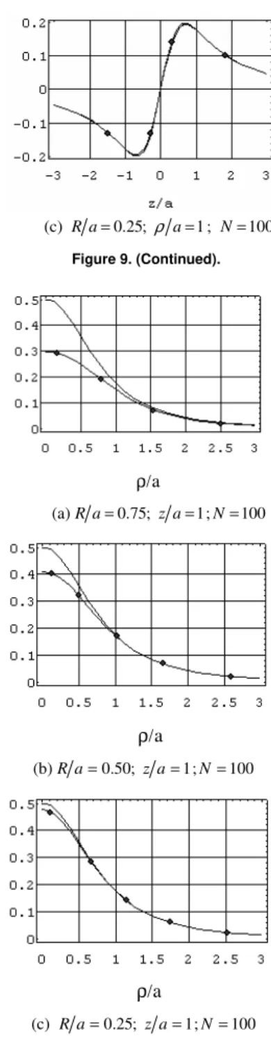
Figures 9 and 10 show the non-dimensional potential calculated for the three cases exemplified, compared to the exact solution given by Eq.(53). We have taken ρ/a=1 and z/a=1 respectively. Notice that agreement is improved drastically as R/a decreases. In fact, as a vortex ring is kinematically equivalent to a surface distribution of dipoles with uniform density, this latter shrinks to a single dipole as R/a→0, what represents exactly the potential flow around an advancing sphere. Figure 11 shows the non-dimensional potential calculated on the sphere surface.
Remarkable is also the fact, in the present problem, that the error in the added mass coefficient is exactly the square of the error norm in the approximate potential solution.
Table 1 Non-dimensional Added Mass Coefficient for a Sphere by a Variational Method. One Vortex Ring at mid-plane.
a
R q a11 δa11 (%) δφ (%) 0.75 2.98 0.42 16.26 40.32
0.50 7.76 0.48 3.05 17.46
0.25 31.94 0.50 0.19 4.34
(a) Ra=0.75; ρ a=1; N=100
(b) R a=0.50; ρ a=1; N=100
Figure 9. Non-dimensional Velocity Potential Function as a function of a
ρ for a Sphere of Radius a by the variational method, compared to the exact solution. Only one Vortex Ring as ‘Trial Function’.
6
A standard convergence analysis was done, following the same approach described in section 3. For the sphere problem, convergence is very fast and a smaller number of terms could have been used, without changing the results. As a matter of fact, for small radius vortex-rings, results are always improved, irrespective additional terms taken in the series, since the asymptotic behavior of the trial function recovers that of a dipole as the radius tends to zero. The use of large radii rings require a larger set of trial functions to perform the same task.
(c) Ra=0.25; ρ a=1; N=100
Figure 9. (Continued).
ξξξξξξξξ ρ/ξξξξξξξξa
ρ/a
(a)R a=0.75; za=1;N=100
ρ/a
ρ/a
(b)Ra=0.50; za=1;N=100
ρ/a
ρ/a
(c) R a=0.25; za=1;N=100
Figure 10. Non-dimensional Velocity Potential Function as a function of a
z for a Sphere of Radius: variational method (♦♦♦♦) compared to the exact solution. Only one Vortex Ring.
(a) R a=0.75;ρ2+z2=a2;N=100
(b) R a=0.50;ρ2+z2=a2;N=100
(c) R a=0.25;ρ2+z2=a2;N=100
Figure 11. (Continued).
Variational Solution for a Family of Spheroids
A rather general form, for which comparable analytical solutions are available, are ellipsoids. Particularly, spheroids or ellipsoids of revolutions, being b the semi-diameter and a on the axis of revolution z. Examples will be shown for oblate spheroids
(
ab<1)
; Figure 12.Table 2 shows the numerical results obtained for the added mass of an oblate spheroid advancing in unbounded inviscid fluid along the revolution axis. Paradigms have been extracted from Newman, 1978, page 147, up to two significant figures. Two aspect ratios have been chosen (a b=0.6;0.2). N is the number of terms used in the series expansions. For the first case (ab=0.6) only one trial function, composed by just one complete circular vortex ring placed on the plane z=0, normal to the axis of revolution, has been used, with non-dimensional radius R b=0.15. Convergence towards the paradigm (0.56) is reached with N≥10. For the second case
) 2 . 0
(ab= , two trial functions, composed by complete circular vortex rings, placed on the plane z=0, with R a=0.15and0.30 respectively, have been used. Convergence is achieved for N≥30. Notice that the vortex ring has been able to reproduce quite well the flow around large curvatures corresponding to small non-dimensional values ab.
Figure 12. Oblate Spheroid (ab=0.6) ; a is the semi-diameter of revolution.
Table 2. Non-dimensional Added Mass Coefficients for an Oblate Spheroid advancing along its axis of revolution. (a is the semi-axis of revolution)
3 33 33
3
4 b
m a
πρ
=
a/b NTF R/b N=5 N=10 N=30 N=50
Paradigm, (Newman) 0.6 1 0.15 0.565 0.564 0.564 - 0.56 0.2 2 0.15;0.30 1.780 0.790 0.621 0.618 0.61
Figure 13. Oblate Spheroid: (a) a system of one pair of complete rings (2ππππ
-rings) for a spheroid advancing along the revolution axis; (b) a system of one pair of counter-rotating semi-circular vortex ring (ππππ-rings) for a rotation around a diameter axis.
0 0,05 0,1 0,15 0,2
0 2 4 6 8 10 12
N
a
4
4
Figure 14. Convergence Rate as a function of the number of terms in the series expansions for the added moment of inertia coefficient for an oblate spheroid (a b=0.6)
Table 3 presents the added moment of inertia coefficient corresponding to rotation about any diameter (the b-axis) normal to the axis of revolution. Results are presented only for the first case
) 6 . 0
(ab= . A system of two pairs of counter-rotating semi-circular vortex rings (α=π), with Rb=0.15and0.30, placed on the plane z=0, has been used as the set of trial functions (NTF =2). Figure 13b illustrates the case of just one pair of counter-rotating
Table 3. Non-dimensional Added Moment of Inertia Coefficient for an Oblate Spheroid. (a/b=0.6).
5 55 55 44
15
8 b
m a a
ρπ =
= for rotation about b-axis.
TF
N R/b N=1 N=5 N=8 N=10 N=12 (Newman) Paradigm
2 0.15; 0.30 0.194 0.094 0.089 0.087 0.086 0.082
It should be noticed that, in general, the use of circular vortex rings does not increase the computational effort significantly, unless they are placed too close to the body surface, when convergence is slow. Results obtained in the paper were intended for validation of the trial function only. Computations of the Hypergeometric functions were therefore performed through the software Mathematica®, which requires somewhat long computational time. A detailed evaluation of computational effort was not intended at this stage.
Other Possible Applications in Unbounded Flow
Many other applications in unbounded potential flow may be devised. An interesting example is the potential flow around a streamlined body, as a submarine. Figure 15a shows the streamlines on the fore-body of a typical submarine. This result was obtained with a set of trial functions composed by poles, dipoles, as well as by lines of poles and dipoles, positioned inside the body surface; Pesce et al., 1997. The yellow line marks the transition to turbulence of the boundary-layer, determined by the classical method of Michel, after post-processing the potential flow that was obtained by the variational method. Figure 15b shows a typical cross-section of the submarine and a possible set of α−rings, suitable to represent the flow around the upper and lower body.
Side view Front
view
(a)
(b)
Figure 15. Flow around a typical submarine fore-body: (a) stream-lines (line marks the transition of the boundary-layer to turbulence, determined by the classical method of Michel); (b) a typical cross-section of the submarine and a possible set of αααα-rings, suitable to represent the flow around the upper and lower body.
The variational method can be also applied to other complex problems, like the surface wave interaction with multiple bodies. The free-surface boundary condition can then be enforced for trial-functions composed by elementary unbounded fluid potentials, like the α−rings family, through a convenient combination of these functions and their normal derivatives with respect to the free-surface; see Aranha & Pesce, 1990.
Another further sought application of the α−rings family is to the classical hydrodynamic impact of a body against the free-surface; see, e.g., Korobkin and Pukhnachov, 1988. This is, however, a highly transient and geometrically non-linear potential flow phenomenon, in which jets (or sprays) are formed along the rapidly marching intersection line that exists between the wetted surface of the body and the free surface; see, e.g., Korobkin and Scolan, 2006. To compute the hydrodynamic impacting force on the body, the added mass tensor has to be properly defined and determined as a function of the penetration of the body into the formerly quiescent free-surface. Analytical mechanics approaches may be rather useful in this case, see, e.g., Pesce, 2003, Cointe et al, 2004 or Casetta and Pesce, 2006.
C
∂ jet
jet root
body jet
free surface J
v vJ
W
Figure 16. The impact of a rigid body against a liquid free surface. Jets or sprays are formed. ∂c indicates the instantaneous position of jet's root, across which there is a flux of kinetic energy and mass.
It should be also pointed out that the main application envisaged for the present method is to deal with zero-lift 3D flows with free-surface, mainly for offshore applications. Nonetheless, lifting flows could also be sought as possible further applications. An encouraging example may be found in Burr, 1993, who successfully addressed the two-dimensional lifting problem, through the variational approach, by a proper implementation of the classical Kutta condition.
Conclusions
An explicit formula for the velocity potential describing a family of vortex-rings in unbounded fluid was firstly derived. The special family is composed by circular-sector rings or ‘α−α−α−α−rings’, i.e., rings that are positioned on the border of a circular sector with aperture angle α. An obvious particular case is the well-known circular vortex-ring. The formula is given in terms of a uniformly valid series involving trigonometric and Hypergeometric functions. The convergence of the series was discussed, proper analytic continuations constructed and asymptotic behaviors recovered. The series can also be expressed in terms of the incomplete Beta function.
Results concerning the complete circular ring were compared to the well known closed solution formula given in terms of Bessel functions with perfect agreement, even recovering the potential jump that occurs by trespassing the barrier potential formed by the ring itself. Graphical examples were shown for various rings of different sector angles. Numerical results for arbitrary α-angles have been verified, by recovering the complete circular vortex ring potential through the finite sum of a sequence of 2
π
K-rings.Finally, as a simple application, the potential flow around three-dimensional bodies was formulated and solved under a variational approach. The method was numerically validated by comparison with results for a sphere and for a family of spheroids. A unique ‘trial function’ corresponding to a circular vortex-ring recovers the advancing sphere potential with excellent results, as expected. Simple systems of rings and α−rings were used as trial-functions sets to compute the solution for a family of spheroids, either for the advancing or rotating cases.
Some other complex problems were devised as possible further applications.
Appendix A - Alternative Expressions forfn(σ)
Take, in the complex plane,t=u2 σ2, such that t=rei(θ+2kπ) and so t12 =−r12eiθ2. The integral
(
)
∫
+ + + 1 0 2 3 2 2 1 = ) ( du u u f n n n σ σ (A1) transforms into( )
∫
+ + + + − 2 1 0 2 3 2 2 3 2 1 2 2 1 ) 1 ( ) ( ) ( 2 1 = ) ( σ σ σ σ dr r r f n n n n n n (A2).Now, taking r=−v the integral reads
( )
∫
− + + + − − − 2 1 0 2 3 2 2 2 3 2 1 2 2 1 ) 1 ( ) 1 ( ) ( ) ( 2 1 -= ) ( σ σ σ σ dv v v f n n n n n n n (A3),that can be written
)) 2 1 ( , 1 2 , 1 ( ) 1 ( ) 1 ( ) ( ) ( 2 1 -= )
( 2 2
2 3 2 1 2 2 + − + − − − + + n n B
f n n
n n n σ σ σ σ (A4)
where =
∫
− − −z q p d q p z B 0 1 1 ) 1 ( ) , ,
( ϑ ϑ ϑ is the incomplete Beta
function. Then from the identity (see, for instance, Erdélyi et al., section 2.5.3), ) , 1 ; 1 , ( ) , ,
( F p q p z
p z q p z B p + − = (A5),
where F(a,b;c,z)=2F1(a,b;c;z) is the Hypergeometric function, it follows that ) 1 ; 2 2 ; 2 3 , 2 1 ( ) ( 1 n + 2 2 = ) ( 2 2 3 2 σ σ
σ + F +n +n +n −
f
n
n (A6).
The Gauss Hypergeometric series is convergent if z<1, that is, in the present case, for σ >1. Notice also that
1 1 ) 1 ( ) , ,
(z pq =zp− −z q− z
B ∂
∂ (A7).
Appendix B - Alternative Expressions forfn(σ)
Analytic Continuation of F(1++++n 2,32++++n;2++++n 2;−−−−σσσσ−−−−2)
Formula (6), section 2.10 in Erdélyi et al., provides the analytic continuation of F(1+n 2,32+n;2+n2;−σ−2) valid for all n. In fact, from ) ) 1 ( ; ; , ( ) 1 ( ) ) 1 ( ; ; , ( ) 1 ( ) ; ; , , ( − − − = = − − − = − − z z c a c b F z z z c b c a F z z c c b a F b a (B1)
we get, in the present case,
) ) 1 ( 1 ; 2 2 ; 1 , 2 3 ( ) 1 ( ) ) 1 ( 1 ; 2 2 ; 2 2 1 , 2 1 ( ) 1 ( ) ; 2 2 ; 2 3 , 2 1 ( 2 2 2 σ σ σ + + + − = = + + − + − = = − + + + − − − n n F z n n n F z n n n F b a (B2)
that not only provides a proper analytic continuation but is always convergent, for all σ≠0.
Alternatively, noticing that c−a=1 in the present case, we could construct the analytic continuation from the incomplete Beta function (see Erdélyi et al., section 2.5.5).
Analytic Continuation of F(1++++n 2,32++++n;2++++n 2;−−−−σ−−−−2) for σ<1
A restrict form for the analytic continuation, valid only for 1
<
σ , is, alternatively, got from Barnes integral (see, e.g. Carrier, Krook & Pierson, section 5.3 (5-77), or Erdélyi et al, section 2.10 (2), op. cit.). For (b−a) not integer the following analytic continuation can be deduced
) ; 1 ; 1 , ( ) ( ) ; 1 ; 1 , ( ) ( ) ; ; , , ( 1 2 1 1 − − − − + − + − − + + − + − − = z b a b c b F z B z a b a c a F z B z c c b a F b a (B3) Where ) ( ) ( ) ( ) ( and , ) ( ) ( ) ( ) ( 2 1 b c a b a c B a c b a b c B − − = − − = Γ Γ Γ Γ Γ Γ Γ Γ (B4).
2 ) 1 ( 2 1 2
3 + − − = +
=
−a n n n
b is not an integer number either.
So, for n even we have
) ; 2 ) 3 ( ; 2 ) 1 ( , 2 3 ( ) ( ) ; 2 ) 1 ( ; 0 , 2 1 ( ) ( ) ; 2 2 ; 2 3 , 2 1 ( 2 ) 2 3 ( 2 2 ) 2 ( 1 2 σ σ σ σ σ − + + + + − − + = = − + + + + + − n n n F B n n F B c n n n F n n (B5) With
(
) (
)
(
)
(
) (
)
(
1 2) (
(1 )2)
2 ) 1 ( 2 2 and , 2 3 2 ) 1 ( 2 2 2 1 n n n n B n n n B − + + − + = + + + = Γ Γ Γ Γ Γ Γ Γ (B6)
Equations (B5) and (B6) are convergent for σ<1 and constitute, for n even, the analytic continuation of
) ; 2 2 ; 2 3 , 2 1
( +n +n +n −σ−2
F
in the sphere of unitary radius. Notice that for n an odd number,
(
−( +1) 2)
; >0 and Γ(
(1− ) 2)
; >2Γ n n n n ,
have both singular behavior.
Appendix C - Asymptotics for φ(ξ,ζ;α) and Velocity Field
Asymptotics for φ(ξ,ζ;α) when ζ=0
From (22), all terms in the series are null, except when n=0. Equation (17) provides then
+ − = 2 0 1 1 ) , 0 ( ζ ζ ζ ζ ζ f (C1)
so that, in non-dimensional form,
) , 0 ( 4 ) ; , 0
( π 0 ζ
α α ζ
φ = f (C2).
Particularly, π α α φ 4 ) ; 0 , 0
( ± =± (C3).
Asymptotics for φ(ξ,ζ;α)when ζ=0
For
ξ
>
1
, equation (22) gives at ζ =0.1 ; 0 ) ; , 0 ,
(ξ ϕα = ξ>
φ (C4).
The same can be shown to be valid in
ξ
<
1
;
α
<
ϕ
<
2
π
. Nevertheless,α
ϕ
ξ
π
α
±
=
α
ϕ
ξ
φ
±;
<
1;0
<
<
4
)
;
,
0
,
(
(C5).Asymptotics for φ(ξ,ζ;α) when σ= ξ2+ζ2→∞
As F[a,b;c;0]=1, we have
,... 2 , 1 ; ; ) ( 1 ) 2 ( 1 ) ( 2 3
2 →∞ =
+
≈ + n
n f n n σ σ σ (C6)
So that, from (22) and (17)
∞ → + = + −
≈ 2 2
2 ; 1 1 4 ) ; , ,
( σ ξ ζ
σ σ σ ζ π α α ϕ ζ ξ φ (C7)
Writing (C7) in the form
∞ → + = + −
≈ 2 2
2 ; 1 1 1 1 4 ) ; , ,
( σ ξ ζ
σ σ σ ζ π α α ϕ ζ ξ φ (C8)
and expanding (C8) in Taylor series in 1σ it follows at once that
(
+)
= + →∞=
≈ 2 2
2 3 2 2 3 ; 2 4 2 4 ) ; , ,
( σ ξ ζ
ζ ξ ζ π α σ ζ π α α ϕ ζ ξ φ (C9) Velocity Field
The following relation is valid, see Abramowitz & Stegun, 15.2.2, or Erdélyi et al, 1953, section 2.8 (20),
) ; ; , ( ) ( ) ( ) ( ) ; ; ,
( F a kb k c k w
c b a w c b a F dw d k k k k k + + + =
and so, the velocity components in polar cylindrical coordinates are given by − + + × × = − ∞ =
∑
1 2 2 0 2 ) ( ) ; ( ! 2 )! 1 2 ( 1 4 ) , ; , , ( n n n n n nn R nf R
z d df I n n R z R R z v ρ σ ρ ρ ρ σ α ϕ π κ α ϕ ρ ρ (C10a) n n n n n n n n n n z R f I n n R R z z d df I n n R z R R z v + + + + =
∑
∑
∞ = ∞ = ρ σ α ϕ π κ ρ ρ σ α ϕ π κ α ϕ ρ ) ( ) ; ( ! 2 )! 1 2 ( 1 4 ) ; ( ! 2 )! 1 2 ( 1 4 ) , ; , , ( 0 2 2 20 2 (C10b)
n n
n
n n R
f I n n R z R z v ′ + =
∑
∞ = ρ σ α ϕ π κ α ϕ ρϕ ( ; ) ( )
! 2 )! 1 2 ( 4 ) , ; , , ( 0 2 (C10c) with, 1 ) ; 2 3 ; 2 5 , 2 2 ( ) 2 2 ( ) 2 3 )( 2 1 ( ) ( 2 ) 2 ( 1 ) ; 2 2 ; 2 3 , 2 1 ( ) 3 2 ( ) ( 1 ) 2 ( 1 ) ( 2 3 2 2 2 2 > − + + + + + + + + + − + + + + + − = − + − + σ σ σ σ σ σ σ n n n F n n n n n n n F n n d df n n n (C11)
or, if (18a) is used,