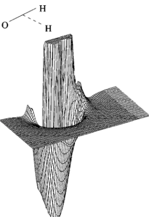
Double-valued potential energy surface for H2O derived from accurate ab initio data and including long-range interactions

Double-valued potential energy surface for H

O derived from accurate

ab initio

data and including long-range interactions

Joa˜o Branda˜o and Carolina M. A. Rio

Quı´mica–Faculdade de Cieˆncias e Tecnologia, Universidade do Algarve–Campus de Gambelas, 8000-117 Faro, Portugal

共Received 18 March 2003; accepted 15 May 2003兲

In a recent work we have been able to model the long-range interactions within the H2O molecule.

Using these long-range energy terms, a complete potential energy surface has been obtained by fitting high-quality ab initio energies to a double-valued functional form in order to describe the crossing between the two lowest-potential-energy surfaces. The two diabatic surfaces are represented using the double many-body expansion model, and the crossing term is represented using a three-body energy function. To warrant a coherent and accurate description for all the dissociation channels we have refitted the potential energy functions for the H2(3⌺u⫹), OH(

2_⌸),

and OH(2⌺) diatomics. To represent the three-body extended Hartree–Fock nonelectrostatic energy terms, V1, V2, and V12, we have chosen a polynomial on the symmetric coordinates times a range

factor in a total of 148 coefficients. Although we have not used spectroscopic data in the fitting procedure, vibrational calculations, performed in this new surface using theDVR3Dprogram suite, show a reasonable agreement with experimental data. We have also done a preliminary quasiclassical trajectory study 共300 K兲. Our rate constant for the reaction O(1D)⫹H2(1⌺g⫹)

→OH(2_⌸)⫹H(2_{S), k(300 K)⫽(0.999⫾0.024)⫻10}⫺10_cm3_molecule⫺1_s⫺1_{, is very close to the}

most recent recommended value. This kinetic result reinforces the importance of the inclusion of the long-range forces when building potential energy surfaces. © 2003 American Institute of Physics. 关DOI: 10.1063/1.1589736兴

I. INTRODUCTION

Although there have been a lot of recent studies on the potential energy surface共PES兲 for the X˜1A1 ground state of

the H2O molecule,1–7the published potential energy surfaces

do not equally cover the bottom of the well and the long-range part of the potential.

Mainly interested in the rovibrational spectra of water, the most recent potential energy surfaces do not reproduce the long-range interactions or use a simplified form to emu-late them, neglecting ‘‘the intramolecular dependence of the atom–diatom dispersion coefficients’’ and the electrostatic quadrupole–quadrupole interaction between the O atom and H2 diatom.

On the other hand, the O(1D)⫹H2(1⌺g⫹)→OH(

2_⌸) ⫹H(2_{S) reaction, which occurs mainly in this system, is}

believed to have a null activation barrier. So the long-range forces between the O atom and H2 diatomic should play an

important role8in the dynamics of this important reaction in atmospheric and combustion chemistry.

Recently9 we have been able to model the long-range interactions between the atoms and diatoms in their ground and first excited states as they appear as fragments in the water dissociation. The computed long-range coefficients, which are a function of the interaction angle and the inter-atomic distance of the diinter-atomic, have been used to build potential energy functions to represent the electrostatic in-duction and dispersion energies within this system.

With this work, we aim to obtain an accurate potential energy surface for this system, covering all configurational

space and the different dissociation channels allowed by spin and symmetry correlation as described by the following equations:

H2O共X˜1A

⬘

→

冦

H2共X˜1⌺g⫹兲⫹O共

1_D兲→2H共2_S兲⫹O共1_{D兲, 共i兲}

H₂共a˜3⌺_u⫹兲⫹O共3P兲→2H共2S兲⫹O共3P兲, 共ii兲 OH共A˜2_{⌺兲⫹H共}2_S兲→2H共2_S兲⫹O共1_D兲, 共i兲

OH共X˜2⌸兲⫹H共2S兲→2H共2S兲⫹O共3P兲. 共ii兲 共1兲

To accomplish it, we used a double-valued functional form10 to represent the two lowest 1A1 surfaces. The

adia-batic surfaces VX and VB are the two eigenvalues of a 2

⫻2 matrix, where the diagonal terms are diabatic surfaces and the nondiagonal term represents the coupling between them. Due to the different dissociation channels and cross-ings of the upper sheet, this potential only reproduces accu-rately the ground-state potential energy surface, VB being an

approximation to the first excited state:

VX/B⫽

冏

冏

冑

Each diabatic surface V1 and V2, is represented within

the double many-body expansion共DMBE兲 framework11and the crossing term V12 is represented using a three-body

en-3148

ergy function. According to the DMBE method each ‘‘many-body energy term’’ is divided as the sum of a short-range term called VEHF,nele (nele stands for nonelectrostatic

en-ergy兲 and a long-range energy term VLR. The first one

ac-counts for the extended Hartree–Fock 共EHF兲 energy, which includes the nondynamical correlation essential for the de-scription of the bond dissociation. The second term includes the dynamic correlation energy, which appears in second-order perturbation theory. However, due to its long-range dependence, the electrostatic and induction energies are sub-tracted from the extended Hartree–Fock energy and included in the V_LRterm. On the other hand, the intra- and inter-intra-atomic correlation terms, which depend on the superposition integrals, are included in the V_EHF,nele energy term.

The three-body terms in this potential have been defined using accurate ab initio data from the literature. To cover some regions of the configurational space where there was a lack of information, we have also done ab initio multicon-figurational self-consistent-field共MCSCF兲 calculations using a triple-␨ basis set augmented with tight and diffuse functions.12

The quality of this new potential energy surface has been assessed with vibrational ab initio calculations and dynami-cal studies using quasiclassidynami-cal trajectories 共QCTs兲.

This article is organized as follows: Section II presents the diatomic potentials we have refitted from accurate ab initio13,14 or Rydberg–Klein–Rees 共RKR兲 spectroscopic data.15 Section III a brief summary of the long-range interactions9used in this potential energy surface. Section IV describes the ab initio points and selection criteria as well as the functional form and numerical approach we used in the fitting procedure. In Sec. V we present a general overview of this surface. In Sec. VI we describe test calculations and comparison with experimental values: in Sec. VI A, prelimi-nary QCT study at 300 K, and in Sec. VI B, the spectroscopic study we have done using theDVR3Dsuite of programs.16In Sec. VII we make some conclusions.

II. DIATOMIC POTENTIALS

To represent the four diatomic potentials resulting from the dissociation of the H₂O ground-state molecule, Eq. 共1兲, we use the EHFACE2U potential model, method III.17Those potentials are constrained to satisfy a normalized kinetic field, and so they have a correct behavior at R→0. Also the VEHF term has a correct asymptotic behavior at R→⬁,

re-producing the leading term for the exchange energy. They also have a dispersion energy term suitably damped.

However, as all the published potentials have different damping functions and functional forms, we have decided to use the diatomic potential for the H2(X˜ 1⌺g⫹) 共Ref. 17兲 and

refitted three of them using the accurate ab initio results of Kołos and Wolniewicz13,14for the H2(a˜3⌺u⫹) and the RKR

experimental data points of Fallon et al.15for both OH (2⌸ and2⌺) diatomic states. We need to use the same damping functions in order to get a coherent representation of the three-body exchange-dispersion energy terms.

The functional form we used to represent the diatomic potentials can be described by

V(2)共R兲⫽V_EHF(2) 共R兲⫹V_dc(2)共R兲, 共3兲

where V_dc(2) is the usual dispersion correlation energy given by Eq. 共4兲.11,18With the exception of the Cn values and the

reduced coordinate␳ in the damping function␹n, this term is the same for all diatomics:

V_dc(2)共R兲⫽⫺

兺

n⫽6,8,10, . . .

Cn␹n共R兲R⫺n. 共4兲

In Eq.共4兲 we use the universal damping functions11,18

␹n共R兲⫽

冋

冉

冊册

and␳ is a reduced coordinate defined by

␳⫽1

2共Rm⫹2.5R0兲, 共8兲

where Rmis the equilibrium diatomic geometry and R0is the

Le Roy19 parameter for the breakdown of the asymptotic expansion of the dispersion energy:

R0共X⫺Y 兲⫽2共

具

2

_典

_具

Y

2

_典

In contrast, the V_EHF(2) functional form has slight varia-tions depending on the particular diatomic and their coeffi-cients have been fitted to reproduce the total potential.

For the H2(3⌺u⫹), we have used the accurate ab initio

results of Kołos and Wolniewicz13,14to fit this potential. To represent the V_EHF(2) term we use the expression

V_EHF(2) 共R兲⫽⫺DRm

冉

兺

冊

冋

兺

册

where X⫽R⫺Rm, R is the internuclear distance in the

di-atomic, Rm is the equilibrium internuclear distance, and

V_excasy m represents the asymptotic exchange energy. This last term is here the symmetric of the one for the singlet state,

V_excasy m共R兲⫽0.805R2.5exp共⫺2.0R兲, 共11兲

and, similarly to the work of Varandas and Dias da Silva,17 the asymptotic exchange energy is damped by the function

␹exc, which is approximated by the universal damping

func-tion 关Eq. 共5兲兴 using n⫽6,␹6.

In addition, to guide the potential at very short distances we have calculated two new points at the MCSCF level.

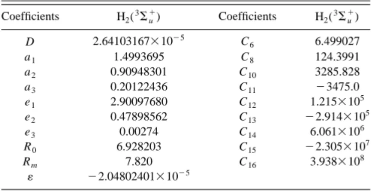
The calculations have been made using the suite pro-gramsGAMESS共Ref. 20兲 and augmented triple-␨quality basis set: (5s2 p1d/3s2 p1d) with diffuse (1s1 p1d) functions.12 To compare our calculations with the literature results13,14we have made a set of calculations at other internuclear dis-tances. In Fig. 1, we present seven points共䉭兲 we have cal-culated. This figure shows the comparison with the literature data共䊊兲. The two types of results are very close. The points we have used in the fitting procedure to obtain this diatomic potential are quoted in the Table I.

The coefficients that define the complete potential for H₂(3_⌺

u

⫹_{), Eqs. 共4兲 and 共10兲, are quoted in Table II, and} Fig. 1 displays the potential.

For OH, states2_{⌸ and}2_{⌺, we have done a fitting}

pro-cedure similar to that of Varandas and Voronin21to the RKR spectroscopic data.15The asymptotic exchange term has been taken from that work,21 and the dispersion coefficients have been semiempirically estimated from polarizability data in a way similar to previous work.9For completeness, we display the functional form for the V_EHF(2) expression21

V_EHF(2) 共R兲⫽⫺DRm

冉

兺

冊

V_excasy m共R兲⫽⫺A˜R␣˜共1⫹a˜R兲exp共⫺␥˜ R兲, 共14兲

and the remaining terms have the same meaning as in Eq. 共10兲.

Table III quotes the parameters to use in Eqs.共12兲–共14兲 for both states of the OH diatomic, and Fig. 2 shows the diatomic potential for the OH(2⌸).

III. LONG-RANGE INTERACTIONS

An important feature of this new potential energy sur-face for H2O is the ability to accurately reproduce the

long-range interactions between the atoms and diatoms in their ground and first excited states as they appear as fragments in the water dissociation: see Eq.共1兲. The functional forms used to represent those interactions have been described elsewhere.9

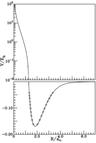
As an example, we present in Fig. 3 a contour plot of the three-body electrostatic energy for an O(1D) atom around a HH(1⌺_g⫹) diatomic.

IV. THREE-BODY EHF ENERGY TERMS A. Input data

Using these long-range energy functions and the accu-rate diatomic potentials, the three-body EHF energy terms for V₁, V₂, and V₁₂, Eq. 共2兲, have been obtained by fitting

FIG. 1. Diatomic potential for H2molecule, 3_⌺

u

⫹_{state共solid line兲. Points:} 䉭, this work; 䊊, literature 共Ref. 13兲, and ⫻, literature 共Ref. 14兲.

TABLE I. Fitted points in the diatomic potential for the H2(3⌺u⫹) molecule.

In column n p we present the number of the used points.

R/a0 V/Eh n p

0.22 3.47321272a ₁

0.30 2.30870248a ₁

1.0↔5.9 Kołos and Wolniewiczb 50 6.0↔12.0 Kołos and Wolniewiczc 30

a

This work.

b_{Reference 13.} c_{Reference 14.}

TABLE II. Coefficients for the diatomic potential of H2(3⌺u⫹).

Coefficients H2(3⌺u⫹) Coefficients H2(3⌺u⫹) D 2.64103167⫻10⫺5 C6 6.499027 a1 1.4993695 C8 124.3991 a2 0.90948301 C10 3285.828 a3 0.20122436 C11 ⫺3475.0 e1 2.90097680 C12 1.215⫻105 e2 0.47898562 C13 ⫺2.914⫻105 e3 0.00274 C14 6.061⫻106 R0 6.928203 C15 ⫺2.305⫻107 Rm 7.820 C16 3.938⫻108 ␧ ⫺2.04802401⫻10⫺5

TABLE III. Coefficients for diatomic potentials of OH molecule, states2⌸ and2⌺. Coefficients OH(2_⌸) OH(2⌺) ⫺D 0.240599442 0.103283115 a1 2.4093609 3.0513954 a2 1.1587677 1.8576639 a3 0.53697044 1.4517489 ␥0 1.8450419 2.1847897 ␥1 2.7809326⫻10 3 4.5080859⫻103 ␥2 5.3432177⫻10⫺5 5.346453⫻10⫺5 m ⫺1 ⫺1 A ˜ 0.307 1.022 ␣ ˜ 1.5 1.5 a ˜ 2.257329 ⫺0.452055 ␥ ˜ 2.0 2.0 R0 6.294894 6.334299622 Rm 1.8344 1.9086 C6 10.00 10.34 C8 180.45 306.8585254 C10 3685.26 6328.709221 ␧ ⫺0.1701493 ⫺0.0929757513

total ab initio energies. Due to the importance of this system, there are a lot of ab initio results in this system. From the published data we decided to use those of Partridge and Schwenke,4 Schneider, Giacomo, and Gianturco,22 and Walch and Harding23 which give a good database for the construction of the PES for the two lower singlet states en-ergy of the H2O molecule. Briefly:

共i兲 Points of Partridge and Schwenke, in 1997 共Ref. 4兲; calculations using a high-quality base set cc- pV5Z, increased with diffuse functions s, p, and d for the

oxygen atom and s and p for the hydrogen atom. These points are henceforth assigned as set 1. 共ii兲 Points of Schneider, Giacomo, and Gianturco, in 1996

共Ref. 22兲; results gotten from a quality base set triple-␨, increased with diffuse functions for the hy-drogen and oxygen atoms. These points are hence-forth assigned as set 2.

共iii兲 Points of Walch and Harding, in 1988 共Ref. 23兲; re-sults obtained from different contractions of the ANO base set 共atomic natural orbitals兲. These points are henceforth assigned as set 3.

All these calculations include the dynamic correlation. Moreover, these energies have been semiempirically cor-rected by the scaled external correlation method24 共SEC兲 to account for the incompleteness of the basis set and higher-order excitation terms.

To minimize the possible inconsistencies between the different sets of data we decided to start from the high-quality points of set 1. We have discarded the points of sets 2 and 3 whose ‘‘distance’’ to any point of set 1 was less than 0.5a0. A similar criterion has been used for sets 2 and 3. In

cases where this ‘‘distance’’ is lower than 0.5a0 only the

points of set 3 have been considered. By ‘‘distance’’ between two points i and j, Di j, we mean the result of the expression

Di j⫽

冑

兺

Also to avoid inconsistencies with our accurate long-range energy term,9 we have discarded those points whose configuration has at least one interatomic distance R1, R2,

or R3 greater than 5.5a0.

As the authors have published only the total interaction energies, the three-body extended Hartree–Fock nonelectro-static term V_EHF,nele(3) was obtained from the total energy for this system subtracting the two-body terms and the three-body dynamic correlation energy as well as the electrostatic and induction energies as modeled in our previous work.9

In regions not covered by those ab initio points we have computed some additional points at the MCSCF level. These calculations have been made with the suite programs

GAMESS 共Ref. 20兲 and using a augmented triple-␨ quality basis set: the above referred basis set for the H atom and (10s5 p3d1 f /4s3 p2d1 f ) augmented with tight functions (2s2 p1d) and diffuse (1s1 p1d1 f ) for the O atom.25 To define the active space for the multiconfiguration calcula-tions we have used all the molecular orbitals generated from the 1s and 2s orbitals of H atom and 1s, 2s, 2 p, 3s, and 3 p orbitals of the O atom. We have considered all configurations generated within this space. Test calculations have shown that a MCSCF calculation within this active space gives lower energy values than a MR–CI 共multireference configuration-interaction兲 with a smaller active space but larger external orbitals. Those points have been corrected to account for the basis-set superposition error.26

B. Fitting procedure

The ground state X1A

⬘

⬘

FIG. 2. Diatomic potential for OH molecule,2_{⌸ state 共solid line兲. Fitted}

points共Ref. 15兲 䊊.

FIG. 3. Contour of three-body electrostatic energy for O(1_{D) atom around}

the HH(1⌺g⫹) diatomic, Vele (3)

. The diatomic has been fixed at the internu-clear distance 1.401a0, with the geometric center in the origin. The contours

are spaced by 0.5mEh and the beginning⫺7.0mEh(O⫽0.0mEh). In this

figure, and in the remaining ones, X and Y are the Cartesian coordinates of the moving atom.

a 2⫻2 matrix. They correspond to two adiabatic surfaces VX

and VB represented by the double-valued functional form,

Eq. 共2兲. These adiabatic surfaces are computed from the di-abatic surfaces V₁ and V₂ and the crossing term V₁₂ that couples them.

Following the work of Murrell et al.,10for the H₂O mol-ecule we can write the two diabatic surfaces

V₁⫽V_O(1)共1_D兲⫹V OH (2)_共2_⌺,R 2兲⫹VOH (2)_共2_⌺,R 3兲 ⫹VHH (2)_共1_⌺ g ⫹_,R 1兲⫹V1(LR) (3) _共R兲⫹V 1(EHF,nele) (3) _共R兲, V₂⫽V_OH(2)共2⌸,R₂兲⫹V_OH(2)共2⌸,R₃兲⫹V_HH(2)共3⌺_u⫹,R₁兲 ⫹V2(LR) (3) _共R兲⫹V 2(EHF,nele) (3) _共R兲, 共16兲 V12⫽V12(EHF,nele) (3) _共R兲,

where V_I(EHF,nele)(3) 共with I⫽1, 2, and 12兲 are the different three-body nonelectrostatic EHF energies terms, and V_1(LR)(3) and V_2(LR)(3) represent the sum of V_ind(3), V_ele(3), and V_dc(3) 共pre-viously defined for each diabatic surface V₁ and V₂).

In order to define the two adiabatic surfaces (V_X and VB), we need to fit three terms: the diabatic surfaces V1 and

V2and the crossing term V12. We used the following

proce-dure:

共i兲 We used the description of the PES of Murrell et al.10 to define the crossing regions.

共ii兲 We considered that in regions far from the crossing, the diabatic surfaces coincide with the adiabatic sur-faces.

共iii兲 We attributed each ab initio point to the diabatic sur-faces V1 and V2. Whenever the point is located near

to the crossing region, where the term of coupling V12

is significant, it will be attributed directly to the sur-face VX or VB.

共iv兲 We have done a preliminary study on the diabatic sur-faces V1 and V2 in order to define the number of

parameters necessary to get a good fit. Whenever nec-essary we have computed additional points.

共v兲 Those preliminary parameters have been used as a starting point for a global fitting where the points at-tributed

共a兲 directly to the V1 共or V2) diabatic surface were

used to fit the function that defines the V₁ 共or V₂) surface and would take value of zero in the fitting to the V₁₂ term and

共b兲 to the VX 共or VB) adiabatic surface were used to fit

the function that defines the VX 共or VB) surface,

that includes the V1 and V2 functions and the

cou-pling term V12.

As described above, we have verified that in some re-gions the information was insufficient to define the true be-havior of the surface and we carried out some calculations for the H2O system. We refer, in particular, the V2 diabatic

surface and the united atom limit on the V1 surface. In this

last case we have estimated the three-body VEHF,nele energy

term from the energy of the united atom limit of O⫹H⫹H 共Ne atom兲 subtracting the energy of the diatomics united atoms共two F atoms and one He atom兲. All these calculations have been done using a basis set with similar quality and using the same active space as for H2O.

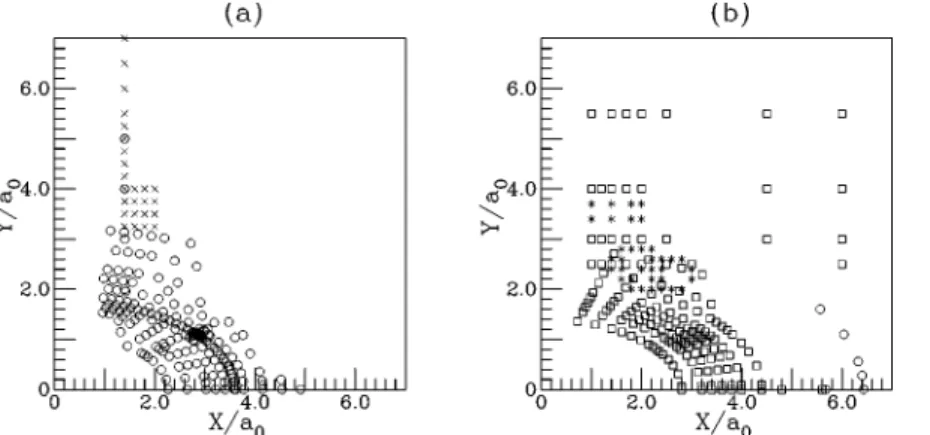
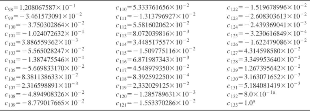
Table IV presents the ab initio points used in the build-ing of this potential energy surface. As an example, we dis-play in Fig. 4 the distribution points used in this fitting for the C2v insertion of the O atom in the H2 diatomic.

The functional form used to represent the nonelectro-static three-body terms, for each term of this potential energy surface, V_I,I⫽1,2,12, can be presented by a product of a poly-nomial form using symmetry coordinates (Q₁, Q₂, and Q₃),27 P, with a range factor D:

V_I(EHF,nele)(3) 共R₁,R₂,R₃兲⫽P_I(3)共Q₁,Q₂,Q₃兲 ⫻DI

(3)_共R

1,R2,R3兲. 共17兲

The use of the D3hsymmetry coordinates is an easy way

to include the permutation symmetry of the H2O system on

FIG. 4. Points distribution used in surfaces V1and V2

calibration for the insertion C2vof the O atom in the H2

diatomic:共a兲 surface V1and 共b兲 surface V2. Legend:

䊊, set 1 共Ref. 4兲; ⫻, set 3 共Ref. 23兲; 䊐, set 2 共Ref. 22兲,

and*, this work. TABLE IV. Origin and number of ab initio points selected for each

compo-nent and global potential.

Set 1a Set 2b Set 3c This work Total

V1 501 152 78 1 732 V2 103 155 21 43 322 VX 184 29 33 - 246 VB - 27 - - 27 Total 788 363 132 44 1327 a_{Reference 4.} b_{Reference 22.} c_{Reference 23.}

the potential energy function. For a system with S2

permu-tation symmetry the polynomials must use only products and powers of the integrity base

Q1, Q3, S2a 2 , S_2b2 , and S₃3, where

冋

⬘

⬘

⬘

册

冋

冑

冑

冑

冑

冑

冑

冑

冑

册

冋

册

and R₁(i), R₂(i), and R₃(i) are a reference geometry for each potential term, whose values are quoted in Table V. For V1

we used as reference the equilibrium position of the water

molecule; for V2 and V12 we found convenient to use C2v geometries whose perimeter is close to the region where those terms should play an important role.

We considered it convenient to use polynomials of de-gree 8 共95 terms兲, 5 共34 terms兲, and 3 共13 terms兲 for the components V1, V2, and V12, respectively, in order to get an

accurate fit avoiding any nonrealistic behavior in regions not covered by the ab initio data. These polynomial terms, used to define the three-body EHF terms, are indicated in the Eqs. 共20兲, 共21兲, and 共22兲: P_1(EHF,nele)(3) ⫽c1⫹c2Q1⫹c3Q3⫹c4Q1 2_⫹c 5S2a 2 _⫹c 6Q1Q3⫹c7S2b 2 _⫹c 8Q1 3_⫹c 9Q1S2a 2 _⫹c 10S3 3_⫹c 11Q1 2_Q 3⫹c12Q1S2b 2 ⫹c13Q3S2a 2 _⫹c 14Q1 4_⫹c 15Q1 2 S2a 2 _⫹c 16S2a 4 _⫹c 17Q1S3 3_⫹c 18Q1 3 Q3⫹c19Q1 2 S2b 2 _⫹c 20Q1Q3S2a 2 _⫹c 21Q3S3 3 ⫹c22S2a 2 S_2b2 ⫹c23Q1 5_⫹c 24Q1 3 S_2a2 ⫹c25Q1S2a 4 _⫹c 26Q1 2 S₃3⫹c27S2a 2 S₃3⫹c28Q1 4 Q3⫹c29Q1 3 S_2b2 ⫹c30Q1 2 Q3S2a 2 ⫹c31Q1Q3S3 3_⫹c 32Q1S2a 2 _S 2b 2 _⫹c 33Q3S2a 4 _⫹c 34S2b 2 _S 3 3_⫹c 35Q1 6_⫹c 36Q1 4_S 2a 2 _⫹c 37Q1 2_S 2a 4 _⫹c 38Q1 3_S 3 3 ⫹c39Q1S3 3 S_2a2 ⫹c40S2a 6 _⫹c 41S3 6_⫹c 42Q1 5 Q3⫹c43Q1 4 S_2b2 ⫹c44Q1 3 Q3S2a 2 _⫹c 45Q1 2 Q3S3 3_⫹c 46Q1 2 S_2a2 S_2b2 ⫹c47Q1Q3S2a 2 _2⫹c 48Q1S3 3_S 2b 2 _⫹c 49Q3S2a 2 _S 3 3_⫹c 50S2b 2 _S 2a 4 _⫹c 51Q1 7_⫹c 52Q1 5_S 2a 2 _⫹c 53Q1 3_S 2a 4 _⫹c 54Q1 4_S 3 3 ⫹c55Q1 2 S_2a2 S₃3⫹c56Q1S2a 6 _⫹c 57Q1S3 6_⫹c 58S3 3 S_2a4 ⫹c59Q3Q1 6_⫹c 60Q3Q1 4 S_2a2 ⫹c61Q3Q1 2 S_2a4 ⫹c62Q1 3 Q3S3 3 ⫹c63Q1Q3S3 3 S_2a2 ⫹c64Q3S2a 6 _⫹c 65Q3S3 6_⫹c 66Q1 5 S_2b2 ⫹c67Q1 3 S_2a2 S_2b2 ⫹c68Q1 2 S₃3S_2b2 ⫹c69Q1S2a 4 S_2b2 ⫹c70S3 3_S 2a 2 _S 2b 2 _⫹c 71Q1 8_⫹c 72Q1 6_S 2a 2 _⫹c 73Q1 4_S 2a 4 _⫹c 74Q1 5_S 3 3_⫹c 75Q1 3_S 3 3_S 2a 2 _⫹c 76Q1 2_S 2a 6 _⫹c 77Q1 2_S 3 6 ⫹c78Q1S3 3 S_2a4 ⫹c79S2a 8 _⫹c 80S3 6 S_2a2 ⫹c81Q1 7 Q3⫹c82Q1 5 Q3S2a 2 _⫹c 83Q1 3 Q3S2a 4 _⫹c 84Q1 4 S₃6⫹c85Q1 2 S₃6S_2a2 ⫹c86Q1Q3S2a 6 _⫹c 87Q1Q3S3 6_⫹c 88Q1 6_S 2b 2 _⫹c 89Q1 4_S 2b 2 _S 2a 2 _⫹c 90Q1 3_S 3 3_S 2b 2 _⫹c 91Q1 2_S 2a 4 _S 2b 2 _⫹c 92Q1S3 3_S 2b 2 _S 2a 2 ⫹c93Q3S3 3 S_2a4 ⫹c94S3 6 S_2b2 ⫹c95S2a 6 S_2b2 , 共20兲 P_2(EHF,nele)(3) ⫽c98⫹c99Q1⫹c100Q3⫹c101Q1 2_⫹c 102S2a 2 _⫹c 103Q1Q3⫹c104S2b 2 _⫹c 105Q1 3_⫹c 106Q1S2a 2 _⫹c 107S3 3_⫹c 108Q1 2 Q3 ⫹c109Q1S2b 2 _⫹c 110Q3S2a 2 _⫹c 111Q1 4_⫹c 112Q1 2 S2a 2 _⫹c 113S2a 4 _⫹c 114Q1S3 3_⫹c 115Q1 3 Q3⫹c116Q1 2 S2b 2 ⫹c117Q1Q3S2a 2 _⫹c 118Q3S3 3_⫹c 119S2a 2 S2b 2 _⫹c 120Q1 5_⫹c 121Q1 3 S2a 2 _⫹c 122Q1S2a 4 _⫹c 123Q1 2 S3 3_⫹c 124S2a 2 S3 3 ⫹c125Q1 4_Q 3⫹c126Q1 3_S 2b 2 _⫹c 126Q1 3_S 2b 2 _⫹c 127Q1 2_Q 3S2a 2 _⫹c 128Q1Q3S3 3_⫹c 129Q1S2a 2 _S 2b 2 _⫹c 130Q3S2a 4 ⫹c131S2b 2 _S 3 3_{, 共21兲} P_12(EHF,nele)(3) ⫽c134⫹c135Q1⫹c136Q3⫹c137Q1 2_⫹c 138S2a 2 _⫹c 139Q1Q3⫹c140S2b 2 _⫹c 141Q1 3_⫹c 142Q1S2a 2 _⫹c 143S3 3_⫹c 144Q1 2_Q 3 ⫹c145Q1S2b 2 _⫹c 146Q3S2a 2 _{. 共22兲}

TABLE V. Reference geometries used on the different elements of matrix

V. Vi R1 (i) R2 (i) R3 (i) V1 2.86194 1.80965 1.80965 V2 4.04 2.717 2.717 V12 3.0 2.6 2.6

TABLE VI. Coefficients for the three-body extended Hartree–Fock energy V1(EHF,nele) (3) term. c1⫽⫺1.565690230⫻10⫺1 c34⫽1.755636267⫻10⫺2 c67⫽⫺2.015458742⫻10⫺1 c2⫽⫺2.544931663⫻10⫺1 c35⫽⫺4.571252263⫻10⫺2 c68⫽6.721735197⫻10⫺2 c3⫽⫺4.876804350⫻10⫺2 c36⫽1.272353899⫻10⫺2 c69⫽1.712406839⫻10⫺1 c4⫽⫺2.690037685⫻10⫺1 c37⫽⫺1.199479525⫻10⫺1 c70⫽6.228997124⫻10⫺2 c5⫽⫺1.535865259⫻10⫺3 c38⫽9.468891942⫻10⫺2 c71⫽⫺3.420843299⫻10⫺4 c6⫽⫺4.890066230⫻10⫺2 c39⫽⫺2.616965983⫻10⫺2 c72⫽1.340173021⫻10⫺2 c7⫽⫺7.329374732⫻10⫺2 c40⫽⫺6.339820029⫻10⫺2 c73⫽⫺4.185837518⫻10⫺2 c8⫽⫺2.109344267⫻10⫺1 c41⫽⫺4.934658276⫻10⫺2 c74⫽⫺1.143824325⫻10⫺2 c9⫽⫺6.445301047⫻10⫺2 c42⫽3.225361439⫻10⫺2 c75⫽3.392045669⫻10⫺2 c10⫽2.411710888⫻10⫺2 c43⫽7.834891306⫻10⫺2 c76⫽8.324394198⫻10⫺2 c11⫽⫺1.555868493⫻10⫺2 c44⫽⫺4.235299197⫻10⫺2 c77⫽⫺8.282447683⫻10⫺3 c12⫽⫺5.607487072⫻10⫺2 c45⫽⫺8.355138053⫻10⫺2 c78⫽⫺7.865970804⫻10⫺2 c13⫽6.202541496⫻10⫺2 c46⫽⫺2.899296365⫻10⫺1 c79⫽⫺2.481027858⫻10⫺2 c14⫽⫺1.429634757⫻10⫺1 c47⫽1.331932799⫻10⫺1 c80⫽⫺1.354741296⫻10⫺2 c15⫽⫺7.444150867⫻10⫺2 c48⫽⫺5.167976333⫻10⫺2 c81⫽⫺5.307323810⫻10⫺3 c16⫽6.156263566⫻10⫺2 c49⫽⫺2.347859542⫻10⫺2 c82⫽⫺9.247430789⫻10⫺3 c17⫽⫺2.245935938⫻10⫺3 c50⫽⫺1.777711260⫻10⫺2 c83⫽2.436516685⫻10⫺2 c18⫽1.330353546⫻10⫺2 c51⫽⫺1.299842803⫻10⫺2 c84⫽⫺3.674205193⫻10⫺3 c19⫽⫺6.788598952⫻10⫺2 c52⫽2.970783506⫻10⫺2 c85⫽3.402165882⫻10⫺3 c20⫽2.271341007⫻10⫺3 c53⫽⫺7.347156570⫻10⫺2 c86⫽1.899518378⫻10⫺2 c21⫽8.980070809⫻10⫺3 c54⫽7.465634301⫻10⫺3 c87⫽⫺1.741461802⫻10⫺2 c22⫽⫺4.986636030⫻10⫺2 c55⫽9.699947247⫻10⫺3 c88⫽1.174832037⫻10⫺3 c23⫽⫺8.429336120⫻10⫺2 c56⫽1.649570767⫻10⫺1 c89⫽⫺5.667240702⫻10⫺2 c24⫽8.978555840⫻10⫺3 c57⫽3.481731649⫻10⫺2 c90⫽⫺7.274439089⫻10⫺3 c25⫽3.568207396⫻10⫺2 c58⫽6.307806127⫻10⫺2 c91⫽9.909591032⫻10⫺2 c26⫽7.898108250⫻10⫺2 c59⫽5.148261697⫻10⫺3 c92⫽⫺7.952480341⫻10⫺2 c27⫽⫺3.299218814⫻10⫺3 c60⫽⫺6.304245065⫻10⫺2 c93⫽⫺3.072103204⫻10⫺3 c28⫽2.266503020⫻10⫺2 c61⫽6.882370932⫻10⫺2 c94⫽1.970459378⫻10⫺3 c29⫽4.924099395⫻10⫺2 c62⫽4.033730863⫻10⫺2 c95⫽⫺2.362856551⫻10⫺2 c30⫽⫺6.192243909⫻10⫺2 c63⫽2.565541551⫻10⫺2 c96⫽8.0⫻10⫺1a c31⫽1.006236871⫻10⫺2 c64⫽⫺6.078121832⫻10⫺2 c97⫽1.0a c32⫽⫺1.067837639⫻10⫺1 c65⫽⫺2.962569550⫻10⫺2 c33⫽1.965447873⫻10⫺2 c66⫽3.084390610⫻10⫺2

a_{This coefficient has been fixed共not fitted兲.}

TABLE VII. Coefficients for the three-body extended Hartree–Fock energy V2(EHF,nele) (3) term. c98⫽1.208067587⫻10⫺1 c110⫽5.333761656⫻10⫺2 c122⫽⫺1.519678996⫻10⫺2 c99⫽⫺3.461573091⫻10⫺2 c111⫽⫺1.313796927⫻10⫺2 c123⫽⫺2.608303613⫻10⫺2 c100⫽⫺3.750302864⫻10⫺2 c112⫽5.581602062⫻10⫺2 c124⫽⫺2.439369041⫻10⫺3 c101⫽⫺1.024072632⫻10⫺1 c113⫽8.072039816⫻10⫺3 c125⫽⫺3.230616849⫻10⫺4 c102⫽3.886559362⫻10⫺3 c114⫽3.448517557⫻10⫺2 c126⫽⫺1.622479086⫻10⫺2 c103⫽⫺5.565028247⫻10⫺2 c115⫽⫺1.509775116⫻10⫺2 c127⫽4.314598580⫻10⫺2 c104⫽⫺1.387475546⫻10⫺1 c116⫽6.871987343⫻10⫺3 c128⫽3.349953640⫻10⫺2 c105⫽⫺5.669833170⫻10⫺2 c117⫽4.548979350⫻10⫺2 c129⫽1.267395642⫻10⫺2 c106⫽8.381138633⫻10⫺2 c118⫽8.392592250⫻10⫺4 c130⫽3.163071652⫻10⫺3 c107⫽2.316598891⫻10⫺3 c119⫽2,332029125⫻10⫺2 c131⫽5.184081419⫻10⫺3 c108⫽⫺4.894908326⫻10⫺2 c120⫽⫺1.285789631⫻10⫺3 c132⫽8.0⫻10⫺1a c109⫽⫺8.779017665⫻10⫺2 c121⫽⫺1.553370286⫻10⫺2 c133⫽1.0a

a_{This coefficient has been fixed共not fitted兲.}

TABLE VIII. Coefficients for the three-body extended Hartree–Fock energy V12(EHF,nele) (3) term. c134⫽⫺1.058457775⫻10⫺1 c139⫽1.103968854⫻10⫺1 c144⫽⫺1.888672360⫻10⫺1 c135⫽⫺2.059102604⫻10⫺2 c140⫽5.152243701⫻10⫺2 c145⫽⫺1.251485382⫻10⫺1 c136⫽6.661037391⫻10⫺2 c141⫽7.878724664⫻10⫺2 c146⫽⫺7.811582863⫻10⫺2 c137⫽⫺6.610026832⫻10⫺2 c142⫽8.313253687⫻10⫺2 c147⫽7.702019726⫻10⫺9 c138⫽1.843067372⫻10⫺2 c143⫽⫺2.827314866⫻10⫺2 c148⫽3.652832367⫻10⫺1

The decay functions we used in terms V1 关Eq. 共23兲兴 and

V2 关Eq. 共24兲兴 are the usual product of hyperbolic tangent

functions. However, the decay for the V12 term 关Eq. 共25兲兴

deserves special attention: instead of a hyperbolic tangent we have used Gaussian functions to cancel this term far from the interest region; for collinear configurations the two diabatic surfaces correlate with states of different symmetry and the coupling term should be zero, which is accomplished with the term sin(⬔HOH) in Eq. 共25兲; the coupling strength being dependent on the difference between the diabatic surfaces, we have included a Gaussian term function of that differ-ence: D1 (3)_{共R兲⫽兵} 1⫺tanh关共R1⫺R1 (1)_兲c 96兴其兵1⫺tanh关共R2 ⫺R2 (1)_兲c 97兴其兵1⫺tanh关共R3⫺R3 (1)_兲c 97兴其, 共23兲 D₂(3)共R兲⫽兵1⫺tanh关共R₁⫺R₁(2)兲c₁₃₂兴其兵1⫺tanh关共R₂ ⫺R2 (2)_兲c 133兴其兵1⫺tanh关共R3⫺R3 (2)_兲c 133兴其, 共24兲 D12 (3)_{共R兲⫽sin共⬔HOH兲exp关⫺100共V} 1⫺V2兲2兴 ⫻exp关⫺c147„共R1⫺R1 (12)_兲2_…兴 ⫻exp关⫺c148„共R2⫹R3⫺2R3 (12)_兲2_{…兴. 共25兲}

Similar to the definition of the symmetry coordinates Q_i, in Eq. 共18兲, in the decay functions 共23兲, 共24兲, and 共25兲 we use a displacement from the same reference geometry.

To warrant a good description to the region closed to the equilibrium geometry of the water molecule, we used a gen-eral weighting function, Eq. 共26兲, to the points assigned to V1, where w˜ and Ere f assume the values 6000 and

0.3704Eh, respectively: Wi⫽ w ˜

冑

Additionally, we multiply this weight by a factor of 200 if the configuration is close to this minimum—i.e., if it sat-isfies the condition expressed by Eq.共27兲:

冑

兺

3

关共Ri⫺Ri

(1)_兲2_兴⬍0.5a

0. 共27兲

Similarly, for the points assigned to V2, VX, VB, and

V12we used Eq.共26兲 where w˜ assumes the values 50, 100, 1,

and 10, respectively. Only for V2points has the value of Ere f

been changed to 0.172Eh. This value corresponds to the

av-erage between the minimum of two diatomics, H2(1⌺g⫹) and

OH(2⌸), respectively, 0.17447Ehand 0.1702Eh. During the

fitting procedure special weights have been assigned to se-lected points.

The coefficient values we have obtained on the final fit are quoted in Tables VI, VII, and VIII.

V. GENERAL OVERVIEW OF A NEW PES

In Table IX we present the geometry of the stable mini-mum of the water molecule, obtained from this surface and from some of the most recent published potentials. Table X quotes the force constants of this potential. Both tables

com-FIG. 5. Contour plot of diabatic surfaces V1in H2O molecule, for H atom

moving around an OH (1.7444a0⭐RO – H⭐1.9444a0) and the center of the

bond fixed at the origin. Contours are equally spaced by 0.02Eh, starting at

⫺0.3704Eh.

FIG. 6. Contour plot of diabatic surface V2in H2O molecule, for H atom

moving around an OH (1.7444a0⭐RO – H⭐1.9444a0) and the center of the

bond fixed at the origin. Contours are equally spaced by 0.02Eh, starting at

⫺0.3704Eh.

TABLE IX. Minimum C2vfor the water molecule.

Prop. This work PJTa _PS1b _PS2c _Expt.d

RHH 2.860831 2.86261719 2.86185923 2.86156774 2.86193768

ROH 1.809798 1.81020726 1.81158582 1.80977168 1.80965

⬔HOH 104.4407 104.499647 104.348 104.481 104.51008

a_{Reference 2.}

b_{Reference 4, only considering the ab initio fit.} c_{Reference 4, considering the total potential.} d

See Refs. 16 and 21 from Murrell et al.共Ref. 10兲.

TABLE X. Spectroscopic properties for the water molecule.

Prop. This work Expt.a

De ⫺0.370401 ⫺0.3704

F11 0.542449 0.542747

F_␣␣ 0.162052 0.160559

F12 ⫺0.292350⫻10⫺2 ⫺0.6423⫻10⫺2

F1␣ 0.314402⫻10⫺1 0.26703⫻10⫺1 a_{See Refs. 16 and 21 from Murrell et al.共Ref. 10兲.}

pare the predicted values with experiment showing a good agreement. Note that this potential and the entry under PS1 don’t use any experimental data in their calibration.

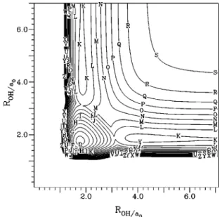
Figures 5 and 6 show the contour plots for the V1and V2

diabatic surfaces, for a H atom moving around an equilib-rium OH molecule, while Figs. 7 and 8 plot the same con-figuration for the adiabatic surfaces X and B, respectively. A perspective view for this configuration on the ground state surface is shown in Fig. 9. From these figures the crossing between these diabatic surfaces is apparent particularly at the collinear geometries where the coupling term vanishes. It is important to notice the saddle point for the isomerization of H₂O, 11 346 cm⫺1 above the bottom well 共this value does not include any correction: see point共1兲 in Table XI兲, which plays an important role in the vibrational spectra and dynam-ics of a high-energy H2O molecule.28 This point is best

viewed as a minimum in Fig. 10 where we plot the collinear stretching of the two H atoms on the ground-state surface. This figure clearly shows the crossing at these geometries of surface V1, H2O(1⌺⫹) state, shown in Fig. 11 and surface

V2, H2O(1⌸) state, shown in Fig. 12. Point 共2兲 of the above

referred table, shown in Figs. 10 and 12 as a minimum, is also a saddle point for the isomerization for large OH values, on a van der Waals region of the H2O(1⌸) surface before the

crossing with the (1_⌺⫹_{) surface, and it is not apparent in}

Fig. 7.

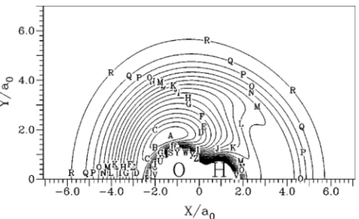
Another interesting view of this surface is the approach of a O(1_{D) atom to an equilibrium H}

2(1⌺g⫹) shown as a

contour plot in Fig. 13 and in a perspective view in Fig. 14. This approach plays an important role on the reaction O(1D)⫹H2(1⌺g⫹)→OH(2⌸)⫹H(2S). The main feature we

can see in this figure is the null activation barrier of this approach. The special contours give us a closer view where we can see a small van der Waals minimum and a small saddle point under the dissociation limit for the C_2v inser-tion, points共3兲 and 共4兲 of Table XI.

In the work of Walch and Harding,23 they obtained a smaller barrier (⬍0.2 kcal/mol) to collinear addition (1⌺⫹ surface兲 and did not find a barrier to edge-on insertion (1A

⬘

VI. PRELIMINARY STUDIES OF THIS PES

We have done same preliminary studies in order to test the PES here presented. We present a QCT study at 300 K, where we compare these results with experimental data ob-tained from the literature and other surfaces. Those prelimi-nary studies allow us to survey some characteristics and the

FIG. 7. Contour plot of H2O (X1A⬘) new PES, for H atom moving around

an OH (1.7444a0⭐RO – H⭐1.9444a0) and the center of the bond fixed at the

origin. Contours are equally spaced by 0.02Eh, starting at⫺0.3704Eh.

FIG. 8. Contour plot of H2O (B 1

A⬘) new PES, for H atom moving around an OH (1.7444a0⭐RO – H⭐1.9444a0) and the center of the bond fixed at the

origin. Contours are equally spaced by 0.02Eh, starting at⫺0.3704Eh.

FIG. 9. Perspective view of H2O (X1A⬘) new PES, for H atom moving

around an OH (1.7444a0⭐RO – H⭐1.9444a0).

TABLE XI. Geometries and energies of metastable minima and saddle points for the new surface.

Pointa R1 R2 R3 ⬔HOH V

共1兲 3.5230500 1.7539662 1.7690838 180.0 ⫺0.3187002

共2兲 5.9690555 4.1150065 1.8540490 180.0 ⫺0.1758476

共3兲 1.41124 4.7430591 4.7430591 17.11119 ⫺0.1036791

共4兲 1.4132597 4.4834532 4.4834532 18.13621 ⫺0.1036700

quality of this new potential energy surface for H2O

mol-ecule, in particular the long-range region that should play an important role in this reaction. Although we have not used spectroscopic information in the fitting procedure, we have also done a vibrational spectroscopic study to compare the predictions of our PES with others and experiment.

A. QCT study at 300 K

The O(1D)⫹H2(1⌺g⫹)→OH(

2_⌸)⫹H(2_{S) reaction is}

believed to have a null activation barrier. So the long-range forces between the O atom and the H2 diatomic should play

an important role on the dynamics of this important reaction in atmospheric and combustion chemistry.

The thermal rate constant at 300 K, for which there are more accurate data in literature has been computed using quasiclassical trajectory dynamic studies on the new H2O

potential energy surface. It has been shown that due to the electrostatic coupling between the ⌺ and ⌸ states of lower energy at linear configurations, higher surfaces should con-tribute about 10%共Ref. 29兲 to the cross section at this tem-perature.

Using a batch of 5000 trajectories we estimate for the thermal rate constant a value of 0.999⫾0.024⫻10⫺10 cm3molecule⫺1s⫺1. Taking into account that correction we estimate the value of 1.1⫻10⫺10cm3molecule⫺1s⫺1, in ex-cellent agreement with the recommended values for k(300 K)⫻1010 共in cm3molecule⫺1s⫺1) of 1.1⫾0.1 共Ref. 30兲, 1.2⫾0.1 共Ref. 31兲, and 1.1⫾0.1 共Ref. 32兲 共for a range of temperatures between 200 K and 350 K兲. Comparing with results from other potential energy surfaces, we found in the literature several values for that rate constant at the same

FIG. 10. Contours for collinear H–O–H geometries of the H2O ground

state. The asymptotic channel is OH(2_{⌸)⫹H. Contours are equally spaced}

by 0.02Eh, starting at⫺0.3704Eh.

FIG. 11. Contours for the term V1H2O(

1_⌺⫹_{) at the same geometry as in}

Fig. 10. The asymptotic channel is OH(2_⌺⫹_{)⫹H. Contours are equally}

spaced by 0.02Eh, starting at⫺0.3704Eh.

FIG. 12. Contours for the term V2H2O(1⌸) at the same geometry as in Fig.

10. The asymptotic channel is OH(2_{⌸)⫹H. Contours are equally spaced by}

0.02Eh, starting at⫺0.3704Eh.

FIG. 13. Contour plot of H2O (X1A⬘) new PES, for O atom moving around

an H2(1.311a0⭐RH – H⭐1.511a0) and the center of the bond fixed at the

origin. Contours are equally spaced by 0.02Eh, starting at⫺0.3704Eh;

dashed contours are equally spaced by 0.1 kcal/mol, the contour labeled by f corresponds to the dissociation energy.

temperature. In particular, we quote for k(300 K)⫻1010 the values of 0.843 in the PES of Schinke and Lester,33 1.63 in the PES of Varandas et al.,8 and 1.3 in the work of Schatz et al.34 共in cm3molecule⫺1s⫺1. Note that those results do not include any contribution from the excited states.

B. Spectroscopic study

We used our PES to carry out some spectroscopic calcu-lations using theDVR3Dsuite of programs.16For this system, H2O, we used Radau coordinates,35,36which are the

appro-priate coordinates for the ABC molecule, where one atom is bigger than the other two.

In Table XII we compare the calculated vibrational lev-els using our PES and using two versions of the potential from Partridge and Schwenke4共PS1 and PS2兲 and the poten-tial of Polyansky, Jensen, and Tennyson2共PJT兲. Those results have been compared to the experimental values obtained in the literature. In conventional notation, ␯1, ␯2, and␯3

rep-resent the symmetric stretching, bending, and antisymmetric stretching, respectively.

Note that the PJT and PS2 potentials have been fitted to accurate spectroscopic data and our PES as well as PS1 use only ab initio data. In the vibrational calculations on the PS

potentials we use the nuclear masses similar to Partridge and Schwenke and in the other calculations we use the atomic masses.

Table XII shows the reasonable results we have obtained with this new potential. This is due to the good quality of the ab initio points used and to the quality of the fitting in the region close to the bottom well.

VII. CONCLUSIONS

The main objective of this work was to build a PES for the water molecule in its fundamental state, H2O(X1A

⬘

this PES we take into account all the dissociation channels allowed by spin symmetry correlation, using the long-range interactions previously defined,9including the atom–diatom anisotropy and their dependence on the diatom coordinate. For the regions of strong interaction we have used ab initio data available in the literature.

We have attributed the ab initio data to the V1 and V2

diabatic surfaces in regions far from the crossing and to the VX and VB adiabatic surfaces in regions where the coupling

term should play an important role. It has been necessary to carry out ab initio calculations for some geometries where the existing information was missing. The two adiabatic sur-faces have been obtained in a global fit to define V1, V2and

the coupling term V12 in a total of 148 parameters.

We have performed quasiclassical trajectories studies in order to assess the importance of the long-range interactions carefully implemented in this PES. The close agreement with experiment reinforces this idea. Calculations of the vibra-tional levels have been done using the new surface. These have been compared with the results on other surfaces and experiment. The agreement obtained owes its quality to the effectiveness of the ab initio points as well as to the fitting procedure.

ACKNOWLEDGMENT

This work was supported by JNICT under the PRAXIS/ PCEX/C/QUI/102/96 research project.

1

T.-S. Ho, T. Hollebeek, H. Rabitz, L. B. Harding, and G. C. Schatz, J. Chem. Phys. 105, 10 472共1996兲.

2_{O. L. Polyansky, P. Jensen, and J. Tennyson, J. Chem. Phys. 105, 6490}

共1996兲.

3_{A. J. C. Varandas, J. Chem. Phys. 105, 3524共1996兲.} 4

H. Partridge and D. W. Schwenke, J. Chem. Phys. 106, 4618共1997兲.

5_{A. J. C. Varandas, J. Chem. Phys. 107, 867共1997兲.}

6_{A. J. Dobbyn and P. J. Knowles, Mol. Phys. 91, 1107共1997兲.}

7_{A. J. C. Varandas, A. I. Voronin, and P. J. S. B. Caridade, J. Chem. Phys.} 108, 7623共1998兲.

8

A. J. C. Varandas, A. I. Voronin, A. Riganelli, and P. J. S. B. Caridade, Chem. Phys. Lett. 278, 325共1997兲.

9_{J. Branda˜o and C. M. A. Rio, Chem. Phys. Lett. 372, 866共2003兲.} 10_{J. N. Murrell, S. Carter, I. M. Mills, and M. F. Guest, Mol. Phys. 42, 605}

共1981兲.

11_{A. J. C. Varandas, Adv. Chem. Phys. 74, 255共1988兲.} 12_{T. H. Dunning, Jr., J. Chem. Phys. 90, 1007共1989兲.}

13_{W. Kołos and L. Wolniewicz, J. Chem. Phys. 43, 2429共1965兲.} 14

W. Kołos and L. Wolniewicz, Chem. Phys. Lett. 24, 457共1974兲.

15

R. J. Fallon, I. Tobias, and J. T. Vanderslice, J. Chem. Phys. 34, 167 共1961兲.

FIG. 14. Perspective view of H2O (X1A⬘) new PES, for O atom moving

around an H2(1.311a0⭐RH – H⭐1.511a0).

TABLE XII. Vibrational levels for different PES of the water molecule. Level This worka _PJTa _PS1a,b _PS2a,c _Expt.d

010 1599.10 1594.68 1597.74 1594.79 1594.74635 020 3165.31 3151.56 3157.80 3151.69 3151.63015 100 3665.28 3657.15 3652.24 3657.08 3657.05325 030 4689.00 4666.61 4676.25 4666.56 4666.7931 002 7446.12 7444.75 7432.60 7445.19 7445.0700

a_{Calculated in this work.} b

Only considered the ab initio fit.

c_{Considered the total fit.} d_{References 19–22 of Ref. 37.}

16_{J. Tennyson, J. R. Henderson, and N. G. Fulton, Comput. Phys. Commun.} 86, 175共1995兲.

17_{A. J. C. Varandas and J. Dias da Silva, J. Chem. Soc., Faraday Trans. 88,}

941共1992兲.

18_{A. J. C. Varandas and J. Branda˜o, Mol. Phys. 45, 857共1982兲.}

19_{R. J. Le Roy, Specialist Periodical Report, Molecular Spectroscopy共The}

Chemical Society, London, 1973兲, p. 113.

20_{M. W. Schmidt, K. K. Baldridge, J. A. Boatz et al., J. Comput. Chem. 14,}

1347共1993兲.

21_{A. J. C. Varandas and A. I. Voronin, Chem. Phys. 194, 91共1995兲.} 22_{F. Schneider, F. D. Giacomo, and F. A. Gianturco, J. Chem. Phys. 104,}

5153共1996兲.

23

S. P. Walch and L. B. Harding, J. Chem. Phys. 88, 7653共1988兲.

24

F. B. Brown and D. G. Truhlar, Chem. Phys. Lett. 117, 307共1985兲.

25_{R. A. Kendall, T. H. Dunning, Jr., and R. J. Harrison, J. Chem. Phys. 96,}

6769共1992兲.

26_{S. F. Boys and F. Bernardi, Mol. Phys. 19, 553共1970兲.} 27

S. Farantos, E. C. Leisegang, J. N. Murrell, K. Sorbie, J. J. C. Teixeira-Dias, and A. J. C. Varandas, Mol. Phys. 34, 947共1977兲.

28_{J. S. Kain, O. L. Polyansky, and J. Tennyson, Chem. Phys. Lett. 317, 365}

共2000兲.

29_{K. Drukker and G. C. Schatz, J. Chem. Phys. 111, 2451共1999兲.} 30_{W. B. DeMore, S. P. Sander, D. M. Golden, R. F. Hampson, M. J. Kurylo,}

C. J. Howard, A. R. Ravishankara, C. E. Kolb, and M. J. Molina,

Chemi-cal Kinetics and PhotochemiChemi-cal Data for Use in Stratospheric Modeling,

JPL Publication No. 97-4, NASA-Jet Propulsion Laboratory, 1997.

31

R. K. Talukdar and A. R. Ravishankara, Chem. Phys. Lett. 253, 177 共1996兲.

32_{R. Atkinson, D. L. Baulch, R. A. Cox, R. F. Hampson, Jr., J. A. Kerr, and}

J. Troe, J. Phys. Chem. Ref. Data 21, 1125共1992兲.

33_{R. Schinke and W. A. Lester, Jr., J. Chem. Phys. 72, 3754共1980兲.} 34_{G. C. Schatz, A. Papaioannou, L. A. Pederson, L. B. Harding, T.}

Holle-beek, T.-S. Ho, and H. Rabitz, J. Chem. Phys. 107, 2340共1997兲.

35_{F. T. Smith, Phys. Rev. Lett. 45, 1157共1980兲.}

36_{B. R. Johnson and W. P. Reinhadt, J. Chem. Phys. 85, 4538共1986兲.} 37_{P. Jensen, S. A. Tashkun, and V. G. Tyuterev, J. Mol. Spectrosc. 168, 271}