www.hydrol-earth-syst-sci.net/19/969/2015/ doi:10.5194/hess-19-969-2015
© Author(s) 2015. CC Attribution 3.0 License.
Development and evaluation of an efficient soil-atmosphere
model (FHAVeT) based on the Ross fast solution of the
Richards equation for bare soil conditions
A.-J. Tinet1,4, A. Chanzy1, I. Braud2, D. Crevoisier3, and F. Lafolie1
1Institut National de la Recherche Agronomique, Unite Mixte de Recherche 1114 Environnement Mediterraneen et
Modelisation des Agro-Hydrosystemes, Site Agroparc, 84914 Avignon CEDEX 9, France
2Irstea HHLY – Hydrology – Hydraulics, Lyon-Villeurbanne, France 3INRA, UMR LISAH (INRA-IRD-SupAgro), 34060 Montpellier, France
4Université de Lorraine, CNRS, CREGU, GeoRessources laboratory, 54518 Vandoeuvre-les-Nancy, France
Correspondence to:A. Chanzy ([email protected])
Received: 2 July 2014 – Published in Hydrol. Earth Syst. Sci. Discuss.: 25 July 2014 Revised: 29 January 2015 – Accepted: 29 January 2015 – Published: 20 February 2015
Abstract.In agricultural management, a good timing in op-erations, such as irrigation or sowing, is essential to enhance both economical and environmental performance. To im-prove such timing, predictive software are of particular inter-est. Optimal decision-software would require process mod-ules which provide robust, efficient and accurate predictions while being based on a minimal amount of parameters eas-ily available. The objective of this study is to assess the ac-curacy of a physically based model with high efficiency. To this aim, this paper develops a coupled model with climatic forcing based on the Ross fast solution for Richards’ equa-tion, heat transfer and detailed surface energy balance. The present study is limited to bare soil, but the impact of vegeta-tion can be easily included. The developed model, FHAVeT (Fast Hydro Atmosphere Vegetation Temperature), is eval-uated against the coupled model based on the Philip and De Vries (1957) description, TEC. The two models were compared for different climatic and soil conditions. More-over, the model allows using various pedotransfer functions. The FHAVeT model showed better performance in regards to mass balance, mostly below 0.002 m, and generally im-proved computation time. In order to allow for a more pre-cise comparison, six time windows were selected. The study demonstrated that the FHAVeT behaviour is quite similar to the TEC behaviour except under some dry conditions. The ability of the models to detect the occurrence of soil
inter-mediate water content thresholds with a 1 day tolerance was also evaluated. Both models agreed in more than 90 % of the cases.
1 Introduction
As explained in the review on decision-making by As-cough et al. (2008), an optimal decision-making software would require process modules which provide robust, effi-cient and accurate predictions while being based on a min-imal amount of easily available parameters. Moreover, a decision-making software should allow for the representation of the major processes occurring in the studied object. In re-gards to decisions based on soil water content for agricultural management, some important processes are the water trans-fers in the soil/plant system and the energy fluxes in the soil and at the surface, the latter being important to determine top boundary conditions from standard climatic data. To repre-sent such processes, characterisation of soil hydraulic prop-erties is a critical point since they are rarely measured at the location of interest and have a strong impact on the simu-lations. The alternative is then to use pedotransfer functions that link those characteristics to commonly measured quan-tities such as the soil textural fractions.
For agricultural management purposes, capacity-based models are generally used (Bergez et al., 2001; Chopart et al., 2007; Lozano and Mateos, 2008). Such conceptual models represent soil through its water storage capacity and vertical fluxes that are governed by an overflow of a compartment to-wards the one just below. In general, additional processes are required to better represent infiltration and upwards flux in-volving empirical parameters that are site specific and need to be calibrated since they are not measurable and thus dif-ficult to address through pedotransfer functions. Moreover, in her work, Blyth (2002) compared a conceptual model to a physically based model. The physically based model showed better performance and more versatility than the concep-tual model. It should be noted, however, that the accuracy of a physically based model is dependent on the modeller’s choice, for instance in regards to parameterisation or chosen processes (Holländer et al., 2014). Therefore, the develop-ment of a versatile, physically based model is of importance to allow for a non-site-specific decision tool.
In the unsaturated zone, a well-known physically based description of the mass balance, in regards to water flow, is the Richards equation. The Richards equation allows for a detailed description of soil water content distribution evolu-tion as well as water fluxes inside the soil domain. Its solu-tion is based on measurable physical parameters such as the water retention and the hydraulic conductivity, which may be obtained through experimentation. Moreover, pedotrans-fer functions are widely developed (Cosby et al., 1984; Rawls and Brakensiek, 1989; Wosten et al., 2001; Schaap et al., 2001) and allow describing of the parameters necessary for the resolution of the Richards equation using soil character-istics such as the soil texture and bulk density. Chanzy et al. (2008) demonstrated that pedotransfer functions may allow for a good approximation for agricultural soil water repre-sentation even though the adequacy of pedotransfer functions close to the surface is still under discussion (Jarvis et al.,
2013), especially for wet conditions when preferential flow occurs.
The Richards equation is highly nonlinear leading to time-consuming numerical resolution and stability issues under some conditions such as the wetting of an initially dry medium. Numerous studies focused on the improvement of the numerical schemes (Short et al., 1995; Zhang et al., 2002; Caviedes-Voullieme et al., 2013) but it should be noted that computing codes based on Richards’ equation are rarely used for decision-making software.
Ross (2003) proposed in his paper a fast solution of the Richards equation. This method demonstrated an accurate, robust and efficient behaviour on a variety of case stud-ies. The solution developed by Ross (2003) has been used in different situations in recent years, proving its efficiency against models based on the classic numerical resolution of the Richards equation and analytical solutions. Varado et al. (2006a) tested the solution to evaluate its efficiency and demonstrated that the model shows improved robustness and accuracy compared to analytical solutions and the model SiSPAT (Braud et al., 1995). In their work, Crevoisier et al. (2009) proposed a comparison of the solution with the Hy-drus software (Simunek et al., 2008) in unfavourable condi-tions, demonstrating an improvement in computing time ef-ficiency and robustness.
Thanks to its efficiency and robustness a model based on Ross’ solution is an interesting choice to develop a decision tool based on soil water content estimation. However, it is important to drive the model with a climate forcing and to be able to have a wide range of soil hydraulic functions (reten-tion curve and soil hydraulic conductivity) in order to profit from the existing pedotransfer functions.
The aim of this paper is to present and evaluate the im-provements made on the model developed in Crevoisier et al. (2009) with the introduction of new soil hydraulic function formalisms as well as new processes (soil heat transfer and surface energy balance). At longer term, the interest would be to enlarge the scope of the soil water and heat transfer model to other processes such as root uptake, solute trans-port, biogeochemical reaction and soil property dynamics. It was found that the main challenge in implementing a physi-cally based model to estimate soil water content is the evalu-ation of soil hydraulic properties, requiring the development of estimation strategies such as using pedotransfer functions (PTF) and assimilation techniques (Witono and Bruckler, 1989; Zhu and Mohanty, 2004; Medina et al., 2014). Our work focuses on the innovation made in the FHAVeT (Fast Hydro Atmosphere Vegetation Temperature) model and does not consider those strategies that are already addressed in other studies (Chanzy et al., 2008). Therefore, to evaluate the FHAVeT model, we used a data set simulated by the TEC model (Chanzy et al., 2008) as our reference. It is based on the DeVries approach, which is physically sound to repre-sent water transfers in the soil and at the soil–atmosphere interface. Moreover, Chanzy et al. (2008) have shown the potential of such a model for operational applications by de-veloping an implementation strategy with limited soil char-acterisation. The question is then to evaluate to which extent the gain in computing efficiency and robustness brought by the Ross method, together with the physical simplification on heat and water coupling, affect the results in comparison to the TEC model that presents a stronger physical background. In this paper, the work is limited to bare soils in order to focus on the impacts of the innovations included in FHAVeT, which are limited to the soil compartment including the inter-face with the atmosphere. Moreover, the very dry conditions encountered near the surface on bare soil are the worst condi-tions in to test the lack of soil water vapour assumption. Bare soil is also an important phase in the crop cycle during which important decisions have to be taken by farmers such as crop installation (soil tillage, sowing).
2 Model description
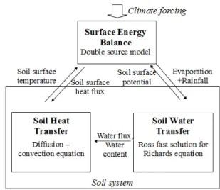
The model FHAVeT consists in the coupling of a surface energy balance, a soil energy balance and a soil mass bal-ance module. Models development and simulations were per-formed using the INRA Virtual Soil1platform. This platform provides an easy way to use and couple numerical modules representing processes occurring in soils. A scheme of the model is presented in Fig. 1. The model consists of three main modules computed sequentially in the following order: surface energy balance – soil water transfer – soil heat
trans-1All information about the platform and how to use it and
con-tribute can be found in the dedicated web site: http://www.inra.fr/ sol_virtuel.
Figure 1.The FHAVeT model coupling scheme.
fer. As shown in Fig. 1 the surface energy balance is driven by climatic forcing, soil surface temperature and soil surface water potential, and it computes evaporation and soil surface heat flux. The soil water transfer module is driven by evap-oration/rainfall and computes soil water potential, water flux and water content. Finally, the soil heat transfer module de-pends on water flux, water content and surface heat flux and computes soil temperature.
2.1 Surface energy balance
An equation of energy budget (Eq. 1) at the soil surface is used to obtain the soil surface heat fluxG(W m−2) and the soil evaporation fluxEg(kg m−2 s−1).
Rng=Hg+Lv(Ts) Eg+G (1)
= −ρacp
(Ta−Ts) RaH
−Lv(Ts)
ρa(ha−hs) Rav
+G (2)
In these equations, Rng (W m−2) is the net radiation, Lv
(J kg−1) is the latent heat of vaporisation andHg(W m−2) is
the sensible heat flux. The aerodynamic resistances for heat and vapourRaH(s m−1) andRav (s m−1) are calculated
us-ing the formulation by Taconet et al. (1986).T corresponds to the temperature andh to the specific humidity (mass of water in air over mass of humid air), subscript “a” relates to the air and subscript “s” to the soil surface level. Moreover, ρa(kg m−3) is the air density andcpthe specific heat at
con-stant pressure. Solving Eq. (1) requires climatic observation parameters, as well as the soil surface temperature and soil surface water potential calculated from the soil heat and wa-ter transfers at the previous time step and input paramewa-ters as described in Table 2.
2.2 Soil mass balance
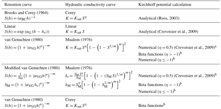
Table 1.Hydraulic property curves available in the FHAVeT and Kirchhoff potential calculation methods.
Retention curve Hydraulic conductivity curve Kirchhoff potential calculation
Brooks and Corey (1964) Corey
S(h)=(αBCh)−λ K=KsatSη Analytical (Ross, 2003)
Linear Linear
S(h)=exp(αG(h−he)) K=KsatS Analytical (Crevoisier et al., 2009)
van Genuchten (1980) Mualem (1976)
S(h)= 1+ |αVGh|n −m
K=KsatSη h
1−
1−S1/m mi2
Numerical (η=0.5) (Crevoisier et al., 2009)a Beta functions (η >−1)b
Numerical (η≤ −1)b
Modified van Genuchten (1980) Mualem (1976)
S(h)=S1
M 1+ |αVGh|
n−m
kr=SMS η kM
h
1−
1−(SMS)1/m mi2
Numerical (η=0.5) (Crevoisier et al., 2009)b
SM= 1+ |αVGhe|n −m
kM=SMη h
1−
1−SM1/m mi2
Beta functions (η >−1)b Numerical (η≤ −1)b
van Genuchten (1980) Corey S(h)= 1+ |αVGh|n
−m
K=KsatSη Beta functionsb
aIntegration method upgraded andbnew feature in the FHAVeT model.
of Ross’ method used in this study is described in Crevoisier et al. (2009). It solves the Richards equation (Eq. 3) by a noniterative approach.
∂θ
∂t = ∇ ·(K∇(eh−z)), (3)
whereθ(m3m−3) is the soil water content,eh(m) is the soil potential,K(m s−1) is the soil hydraulic conductivity andz (m) is the soil depth. A detailed description of the Ross so-lution may be found in Crevoisier et al. (2009). Similarly to the code developed in Crevoisier et al. (2009), a water sur-face layer and time step optimisation are used. The Ross so-lution is based on a linearisation of the mixed form of the Richards equation. The solution evaluates the effective sat-uration (S=(θ−θr)/(θs−θr)) under unsaturated conditions
and Kirchhoff potential (φ (h)= 0 R
−∞
K(eh) dehin m2s−1) un-der saturated conditions to allow for an exact calculation of the Darcian fluxes (Crevoisier et al., 2009). However, the in-tegration of the hydraulic conductivity is not always straight-forward. Ross (2003) used exclusively the Brooks and Corey formulation which is integrable analytically. Crevoisier et al. (2009) developed a numerical integration method for the use of the van Genuchten–Mualem hydraulic characteristics with η=0.5. However, some PTF, including commonly used PTF, require the use of other formulations. For instance, the PTF of Wosten et al. (2001) or Schaap et al. (2001) implies the use of van Genuchten–Mualem hydraulic characteristics with η potentially different from 0.5. To this end, a method using beta functions was developed for the integration of hydraulic
conductivity as described by van Genuchten–Mualem. This method, however, is convergent only forη >−1. Therefore, a numerical iterative method was developed for the usabil-ity of the van Genuchten–Mualem description withη≤ −1. A summary of the hydraulic properties that may be used in FHAVeT is shown in Table 1.
2.3 Soil energy balance
The soil energy balance is modelled using a simple convec-tion diffusion model (Eqs. 4–5) with convecconvec-tion being lim-ited to the liquid phase.
(ρC)eq ∂T
∂t +ρwCwq
σ· ∇T = ∇ ·(λ∇T ), (4)
(ρC)eq=ρhCeq=ρwCwθ+ρsCs(1−θs) , (5)
where ρs (ρw) (kg m−3) is density of solid (water), ρh
(kg m−3) is the soil bulk density, θs (m3m−3) is the
sat-urated water content (assumed equal to the porosity), Cs
(Cw) (J kg−1K−1) is the specific heat of solid (water) and λ(W m−1K−1) is the soil heat conductivity. The soil heat conductivity is assumed to have a linear dependence on soil water content following Eq. (6) (Van de Griend and O’Neill, 1986) where3s (J m−2K−1s−1/2) is the thermal inertia at
saturation.
λ=(1/0.654(3s+2300θ−1890)) /Ceq (6)
Table 2.Input climate forcing and parameters for the FHAVeT model.
Climatic forcing data
Short-wave incoming radiation RG W m−2 Long-wave incoming radiation RA W m−2 Atmospheric temperature at reference heightTa K
Atmospheric pressurepatm Pa
Air vapour contentea Pa
Wind velocity at reference heightUa m s−1
General properties
Water densityρw 1000 kg m−3
Air densityρa kg m−3 Function of temperature and pressure
Latent heat of vaporisationLv J kg−1 Function of temperature
Specific heat of dry air at constant pressurecp 1004 J kg−1K−1
Specific heat of waterCw 4181 J kg−1K−1
Surface energy properties
Ground surface albedoαg 0.20–0.30 Function of surface water content
Ground surface emissivityεg 0.96
Roughness length for momentumzom 0.002 m
Roughness length for heatzoh m Calculated with Brutsaert (1982) formula
Soil hydraulic properties
Saturated volumetric water contentθs m3m−3
Residual volumetric water contentθr m3m−3
Water retention curve parameters Hydraulic conductivity curve parameters
Soil thermal properties
Soil heat conductivityλ W m−1K−1 Function of soil water content Soil heat capacityCλ J kg−1K−1 Function of soil bulk density
2.4 The reference model: TEC
The TEC model (Chanzy and Bruckler, 1993) is based on the heat and mass flow theory in unsaturated media (Philip and De Vries, 1957). The resulting nonlinear partial differen-tial equation system is solved using a Galerkin finite element method. The model is driven by a climatic forcing in case of bare soil. The model was evaluated against various exper-imental conditions (Chanzy and Bruckler, 1993; Aboudare, 2000; Findeling et al., 2003; Sillon et al., 2003). The major differences between the models TEC and FHAVeT are as fol-lows:
– TEC is based on a finite element method for resolution of the equations, while FHAVeT uses the Ross solu-tion for solving mass balance, and the energy balance is solved through a finite difference method;
– the coupling of soil mass and energy balances is based on a tightly coupled Philip and De Vries (1957) ap-proach in TEC while the FHAVeT model uses a loose coupling, neglecting the vapour transport.
There are however others differences between the two models. The evolution of soil heat conductivity with soil wa-ter content and the aerodynamic resistances are calculated through different means. Moreover, the numerical spatial dis-cretisations are different, with a coarser mesh for FHAVeT near the surface.
3 Model intercomparison
(a) Avignon sequence
(b) Estree-Mons sequence
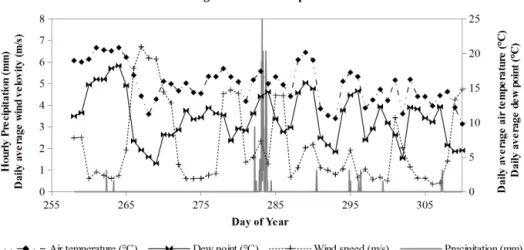
Figure 2.Climate forcing: precipitation, air temperature, dew point and wind velocity at 2 m height.
3.1 Climatic forcing
The cases studied were chosen so as to offer a variety of climatic and soil conditions that may occur in France and in an agronomic context. Two climatic sequences are used. The first one was measured at Avignon (southern France, 43.78◦N, 4.73◦E) and represents a Mediterranean climate
with occasional heavy rains and long periods of dryness (Fig. 2a). Wind velocity also varies strongly. The second climatic sequence was measured at Estrées-Mons (north-ern France, 48.99◦N, 2.99◦E). It represents an oceanic cli-mate with frequent light rainfalls and short dryness periods (Fig. 2b).
In order to study specific features of the two climatic se-quences, six time windows (TWs) were selected (Table 3). TWs 1 and 2 are chosen within the first drying period of the Avignon sequence with TW 1 showing strong wind
condi-tions and TW 2 weak wind condicondi-tions. Indeed, Chanzy and Bruckler (1993) demonstrated that wind has an influence on vapour transport, with lower vapour flow when the convec-tive part of the climatic demand is stronger. TW 3 is selected during the heavy rain period of the Avignon sequence. TW 5 covers the drying conditions of the Estrées-Mons climate. Fi-nally, TWs 4 and 6 were chosen during wet periods of the Estrées-Mons sequence, respectively, before and after the dry period. A summary of the averaged climatic conditions dur-ing the six time periods is shown in Table 3.
3.2 Soil types
Table 3.Climatic forcing summary for the selected time windows (TWs).
Case Site Start date End date Duration Temperature Precipitation Mean wind velocity
TW 1 Avignon 23 Sep 1997 30 Sep 1997 168 h 14.9◦C 0 mm 5.14 m s−1 TW 2 Avignon 30 Sep 1997 5 Oct 1997 120 h 15.3◦C 0 mm 0.65 m s−1 TW 3 Avignon 11 Oct 1997 12 Oct 1997 24 h 15.9◦C 55 mm 1.25 m s−1 TW 4 Mons 4 Oct 2004 8 Oct 2004 91 h 15.9◦C 16 mm 4.08 m s−1 TW 5 Mons 16 Oct 2004 25 Oct 2004 214 h 14.9◦C 1 mm 3.09 m s−1 TW 6 Mons 26 Oct 2004 31 Oct 2004 120 h 12.9◦C 11 mm 3.06 m s−1
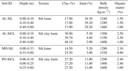
Table 4.Soil characteristics for comparative study, from Chanzy et al. (2008),
Soil ID Depth (m) Texture Clay (%) Sand (%) Bulk Organic density matter (kg m−3) (%)
AL-SiL 0.00–0.10 Silt loam 17.00 34.30 1240 1.50
0.10–0.40 17.00 29.20 1280 1.50
0.40–0.80 17.00 29.20 1460 1.00
AL-SiCL 0.00–0.10 Silt clay loam 38.90 5.30 1300 2.50
0.10–0.40 39.70 4.60 1350 2.50
0.40–0.80 48.10 2.00 1600 1.00
MO-SiL 0.00–0.33 Silt loam 14.50 5.20 1280 2.10
0.33–0.80 25.20 3.00 1520 0.90
PO-SiCL 0.00–0.10 Silt clay loam 27.20 11.00 1290 2.40
0.00–0.25 27.20 11.00 1400 2.40
0.25–0.80 27.20 11.00 1600 1.00
3.3 Soil hydraulic characteristics
To validate the versatility of the model, the three integration methods (Table 1) were solicited through the use of three dif-ferent PTFs. The pedotransfer function developed by Cosby et al. (1984) offers parameters corresponding to a Brooks and Corey set of hydraulic properties and therefore requires the use of analytical integration in the software. The pedo-transfer function developed in Rawls and Brakensiek (1989) allows deriving van Genuchten–Mualem hydraulic property parameters with the hypothesis of shape parameter, other-wise known as tortuosity,η=0.5. Therefore, integration with beta functions may be used. Finally, the pedotransfer func-tion of Wosten et al. (2001) also derives van Genuchten– Mualem parameters, but the shape parametersηobtained are usually below−1; therefore, numerical integration is neces-sary. All three functions require the same parameters, which are the textural characteristics of soils, summarised in Ta-ble 4.
3.4 Soil thermal characteristics
Thermal characteristics of the different soils were consid-ered dependent on volumetric soil water content. The heat
capacity is calculated as the mean of soil and water capacities weighed by relative volumes. In the FHAVeT model, the heat conductivity dependence on the soil water content is obtained through Eq. (6). The thermal inertia at saturation3shas been
tabulated against soil textures by Van de Griend and O’Neill (1986). In the TEC model, the evolution of heat conductivity is obtained through the De Vries (1963) description. 3.5 Model setup
The initial values for soil matric potential and soil tempera-ture used in the FHAVeT model were the ones derived us-ing the TEC model from a preliminary climatic sequence (Chanzy et al., 2008). Constant matric potential (−3.33 m) and temperature (293 K) are considered at the bottom of the studied domain for both models as used in Chanzy et al. (2008).
Figure 3.Maximum absolute error in mass balance (in cubic metres of water per unit of soil surface) – comparison between models. The dotted line corresponds to the 1 : 1 line.
4 Results and discussion 4.1 Models performances
A study on the efficiency of the Ross solution against the classic resolution of Richard’s equation under various bound-ary conditions was done in Crevoisier et al. (2009). In their work, they demonstrated that Ross’ solution allowed for a computation time of 5 times per grid cell faster (on average) compared to a regular solution of Richards’ equation. Simi-lar outcomes, (computation time of around a couple minutes with FHAVeT and a few tens of minutes with TEC) were ob-served in this study. It should be noted that in one case (AL-SiCL with the Wosten pedotransfer functions and under the Avignon climate) the computation time using FHAVeT re-mained in the same order of magnitude, as when using TEC. To compare the numerical accuracy of both models, a calculation of mass balance was performed. The mass bal-ance absolute error was computed as the absolute differ-ence between cumulated inflow and outflow of the soil do-main and the soil water storage evolution from initial state at each time step. The maximal value along time for the mass balance error is represented in Fig. 3. As shown in Fig. 3, the TEC mass balances are not always respected (er-ror lower than 0.01 m3m−2) due to the strong water poten-tial near the surface in dry conditions. FHAVeT offers im-proved results in regards to mass balance compared to the TEC model. In most cases the absolute mass balance error was below 0.002 m3m−2, with only one case being higher. In this particular point, corresponding to the soil AL-SiCL with the Wosten pedotransfer functions and under the Avi-gnon climate, both the computing time and the mass bal-ance (0.008 m3m−2) error were too large. As explained in the model description, the variables calculated are different when a cell is saturated (Kirchhoff potential) or unsaturated (effective saturation). Therefore, when a cell is going from unsaturated to saturated state (or reversely), the calculation undergoes an error. For the hydraulic conductivity curves from Wosten et al. (2001), there is a very steep nonlinear
(a) 0-5cmlayer
(b) 0-30cmlayer
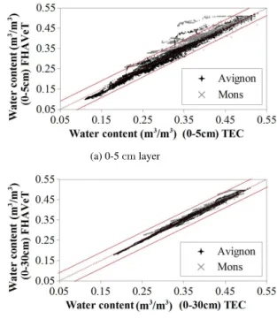
Figure 4. Comparison of soil water content between models FHAVeT and TEC for all models every 2 h.
variation of permeability close to the saturation. This leads to a slow numerical calculation of the permeability close to saturation state as well as a strong discrepancy between the soil’s saturated and slightly unsaturated state flow character-istics. All of these considerations lead to a heightened proba-bility for an “oscillation” to occur between saturated and un-saturated states and the consequent error accumulation. An improvement of the numerical integration method should, however, improve the computation time and allow for the use of a more constraining numerical tolerance.
4.2 Water content evaluation
Figure 4 shows the comparison of all cases studied between soil water content of both models for the 0–5 and 0–30 cm soil layers. A tolerance of 0.04 m3m−3is shown. The models show generally good agreement. For the 0–5 cm layer, only 1.55 % (6.76 %) of the results are out of the tolerance zone for the Avignon (Mons) climate. The results go down to 0 % (1.17 %) for the 0–30 cm layer under the Avignon (Mons) climate.
To study the conditions of the divergences between the two models, the evolution of soil water content with time for the surface layer and in one particular simulation is shown in Fig. 5. This figure shows that the most significant discrep-ancy between the two models seems to occur during TW 5, that is, during the drying period of the Mons climate.
Figure 5.Soil water content evolution in time for the 0–5 cm layer; comparison between models – soil AL-SiL, PTF – Wosten. Avignon climate (top) and Mons climate (bottom).
(a) 0-5cm layer
(b) 0-30cm layer
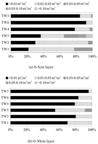
Figure 6.Absolute water content difference distribution between the developed model and TEC for each climatic case study.
(0–5 and 0–30 cm) for both models over each time window. The comparison takes into account all pedotransfer func-tions.
It can be clearly observed that under wet conditions (TWs 3, 4 and 6) the two models led to similar results with the absolute difference in averaged water content being lower than 0.01 m3m−3for around 80 % of the time in the 0–5 cm soil layer and always below 0.03 m3m−3in the 0–30 cm soil layer. However, under dry conditions (TWs 1, 2 and 5) the
Figure 7.Daily evaporation (in mm) evolution in time; comparison between models – Soil AL-SiL, PTF – Wosten.
Figure 8.Water content profiles in TW 2 (dry conditions, Avi-gnon climate, DOY (day of year) 275), TW 5 (dry conditions, Mons climate, DOY 292) and TW 6 (wet conditions, Mons climate, DOY 300) for soil AL-SiL, Wosten pedotransfer function.
difference between the two models is more consequent. This is especially true in TW 5, where there is little rain for a long time (1.5 mm in 12 days), which leads to an absolute water content difference of over 0.1 m3m−3. Since the discrepan-cies between the models mostly occur during drying, the lack of vapour transport is likely to be a source of error. In order to investigate the role of vapour transport, the evaporated flux was plotted in Fig. 7 for one case. This case shows represen-tative behaviour of all soils and climates studied where there is discrepancy between the two models (with the exception of the case showing numerical issues).
surface must be balanced by vapour flow to produce greater evaporation rates. Under Avignon climate, both models led to similar evaporation rates even in very dry conditions and therefore the water content profiles (Fig. 8) are comparable even close to the surface. In such dry conditions, Chanzy (1991) showed that water vapour flows are much smaller than at the beginning of the drying phase. Therefore, intermediate water content conditions, such as the ones encountered un-der Mons climate, lead to the strongest discrepancies. After a rainy period, the profile almost seems to be recovered in TW 6. While the maximal error between the two models in water content is 0.087 m3m−3in the dry state (TW 5), it is 0.015 m3m−38 days later. This result shows that the local error generated during the drying is diluted along the soil profile. Moreover, the error in water amount of the whole domain is reduced by 27 % (from 0.0071 m3m−2in the dry state to 0.0052 m3m−2), showing a partial recovery of soil water content.
4.3 Model ability for water content thresholds estimation
In decision-support software, soil water content thresholds can be applied as criteria for decisions on agronomic man-agement, such as irrigation or tillage and harvesting, to pre-vent soil compaction (Saffih-Hdadi et al., 2009). Therefore, the ability of a model to accurately detect the day when the soil water content status reaches such thresholds is essen-tial. Figure 9 shows the number of dates (considering TEC as a reference) in which a given saturation value (for the top 30 cm layer) was detected either from dry to wet conditions (wetting) or from wet to dry conditions (drying) as well as day detection with a 1 day tolerance.
Due to the small number of saturation condition cases be-low 50 %, the be-lowest threshold shown in Fig. 9 is 60 %. It can be observed that thresholds are detected on the same date in two-thirds of the cases at higher saturation (thresholds of 90 and 80 %) and in slightly over half of the cases for thresh-olds of 70 and 60 % during drying. The success rate is much higher during wetting. Moreover, the success in day detec-tion with a 1 day tolerance is quite high in wet condidetec-tions (thresholds of 90 %).
Important day detection delays (or advance) of over 3 days have occurred in only 0.8 % of the cases and significant day detection misses (when the threshold is reached for more than three days) in 1.4 % of the cases. The day detection in-accuracy may have different causes. The case where mass balance error is high has lead to an early detection in the FHAVeT model. This is likely due to the numerical error as the discrepancy between soil water volume between the two models and the mass balance error in the FHAVeT model are quite similar. The other cause of day detection miss or de-lays could be the lack of vapour transport. Indeed, all other day detection misses or delay appear during the drying riod and especially TW 5. As mentioned previously, this
pe-Figure 9.Day detection success rates. Drying 0day and wetting 0day show the number of identical day detection for both models during drying and wetting respectively. Drying±1 day and wet-ting±1 day show the success rate for day detection when there is less than 1 day difference between the two models.
riod corresponds to the intermediate water condition that led to the largest discrepancy in evaporation and thus soil mois-ture. Therefore, in a tightly coupled model such as TEC, the soil is allowed to dry at a higher pace, leading to earlier day detection than in a loosely coupled model such as FHAVeT.
5 Conclusions
FHAVeT extends the model developed by Ross (2003) and improved by Crevoisier et al. (2009) by introducing a cou-pling with the atmospheric conditions and by considering a wider range of soil hydraulic functions in order to profit from commonly used pedotransfer functions. The coupled model is based on existing process modules and uses the coupling technology offered by the soil virtual modelling platform to make the software development easier. As a consequence, a loose coupling between soil heat and mass flow is introduced leading, to neglect water vapour flows. Moreover, water and heat flow are computed sequentially. The model developed was compared to a reference model, TEC, under two climates typical of France and using four soil textures from different areas in France.
The model demonstrated good efficiency and improved mass balance conservation in comparison to the TEC model with the exception of one particular condition. In that case, the soil characteristic curves (soil water retention and rela-tive permeability) are highly nonlinear and lead to an “oscil-latory” behaviour between saturated and unsaturated states, accumulating numerical errors.
Since the developed model is aimed at being a support for decision-making software, it is important that it accurately simulates threshold criteria. The FHAVeT and TEC models are in good agreement for about 90 % of the day detections with a 1 day tolerance. Considering the modelling param-eters and initial condition uncertainties in field application, such a tolerance seems to be acceptable. Moreover, due to the lesser computing time (Crevoisier et al., 2009) required by the Ross solution, the FHAVeT model is a much better candidate than TEC for improvement techniques of param-eter and initial condition descriptions such as data assimila-tion.
However, under drying conditions, the FHAVeT model may fail to correctly simulate the soil drying, especially close to the surface. In such conditions, wrong decisions may be taken even though the model allowed for a good recovery of the soil water content after a rainy period. It is consequently important to fully identify the specific climatic and soil his-tory conditions that lead to an inaccurate description of the soil behaviour in regards to water content. To do so, a wider evaluation of the model, as well as a comparison with exper-imental field values, requires further work. Future improve-ments of the model include a better numerical integration method in order to deal with highly nonlinear soil charac-teristic functions and coupling with water transfers due to vegetation.
Acknowledgements. The project was funded by project ANR-11-EITC-001 (Agence Nationale de Recherche).
Edited by: N. Romano
References
Aboudare, A.: Stratégies de stockage et d’utilisation de l’eau pour le tournesol pluvial dans la région de Meknes, PhD thesis, Institut Agronomique et Vétérinaire Hassan II, Rabat, Maroc, 2000. Ascough, J., Maier, H., Ravalico, J., and Strudley, M.: Future
re-search challenges for incorporation of uncertainty in environ-mental and ecological decision-making, Ecol. Model., 219, 383– 399, 2008.
Bergez, J.-E., Debaeke, P., Deumier, B., Lacroix, B., Leenhardt, D., Leroy, P., and Wallach, D.: MODERATO: an object-oriented decision tool for designing maize irrigation schedules, Ecol. Model., 137, 43–60, 2001.
Blyth, E.: Modelling soil moisture for a grassland and a woodland site in south-east England, Hydrol. Earth Syst. Sci., 6, 39–48, doi:10.5194/hess-6-39-2002, 2002.
Braud, I., Dantas-Antonino, A., Vauclin, M., Thony, J., and Ruelle, P.: A Simple Soil Plant Atmosphere Transfer model (SiSPAT), J. Hydrol., 166, 213–250, 1995.
Brooks, R. and Corey, A.: Hydraulic properties of porous media, Hydrology Paper 3, Colorado State Univ., Fort Collins, 27 pp., 1964.
Brutsaert, W.: Evaporation into the atmosphere: Theory, history and applications, D. Reidel Publishing Co., Dordrecht, 299 pp., 1982. Caviedes-Voullieme, D., Garcia-Navarro, P., and Murillo, J.: Veri-fication, conservation, stability and efficiency of a finite volume method for the 1D Richards equation, J. Hydrol., 480, 69–84, 2013.
Chanzy, A.: Modélisation simplifiée de l’évaporation d’un sol nu utilisant l’humidité et la température de surface accessible par télédétection, PhD thesis, Institut National Agronomique Paris-Grignon, Paris, France, 1991.
Chanzy, A. and Bruckler, L.: Significance of soil surface moisture with respect to daily bare soil evaporation, Water Resour. Res., 29, 1113–1125, 1993.
Chanzy, A., Mumen, M., and Richard, G.: Accuracy of top soil moisture simulation using a mechanistic model with lim-ited soil characterization, Water Resour. Rese., 44, W03432.1– W03432.16, 2008.
Chopart, J., Mezino, M., Aure, F., Le Mezo, L., Mete, M., and Vau-clin, M.: OSIRI: A simple decision-making tool for monitoring irrigation of small farms in heterogeneous environments, Agr. Water Manage., 87, 128–138, 2007.
Cosby, B., Hornberger, G., Clapp, R., and Ginn, T.: A statistical exploration of the relationship of soil moisture characteristics to the physical properties of soils, Water Resour. Res., 20, 682–690, 1984.
Crevoisier, D., Chanzy, A., and Voltz, M.: Evaluation of the Ross fast solution of Richards’ equation in unfavourable conditions for standard finite element methods, Adv. Water Resour., 32, 936– 947, 2009.
De Vries, D.: Physics of plant environment, in: chap. Thermal prop-erties of soil, North-Holland Publishing Co., the Netherlands, 210–235, 1963.
Evett, S. and Parkin, G.: Advances in soil water content sensing: the continuing maturation of technology and theory, Vadose Zone J., 4, 986–991, 2005.
Evett, S., Schwartz, R., Tolk, J., and Howell, T.: Soil profile wa-ter content dewa-termination: Spatiotemporal variability and neutron probe sensors in access tubes, Vadose Zone J., 8, 926–941, 2009. Findeling, A., Chanzy, A., and de Louvigny, N.: Modeling water and heat flows through a mulch allowing for radiative and long distance convective exchange in the mulch, Water Resour. Res., 39, 1244, doi:10.1029/2002WR001820, 2003.
Haverd, V. and Cuntz, M.: Soil-Litter-Iso: A one-dimensional model for coupled transport of heat, water and stable isotopes in soil with a litter layer and root extraction, J. Hydrol., 388, 438– 455, 2010.
Holländer, H. M., Bormann, H., Blume, T., Buytaert, W., Chirico, G. B., Exbrayat, J.-F., Gustafsson, D., Hölzel, H., Krauße, T., Kraft, P., Stoll, S., Blöschl, G., and Flühler, H.: Impact of modellers’ decisions on hydrological a priori predictions, Hy-drol. Earth Syst. Sci., 18, 2065–2085, doi:10.5194/hess-18-2065-2014, 2014.
Jarvis, N., Koestel, J., Messing, I., Moeys, J., and Lindahl, A.: In-fluence of soil, land use and climatic factors on the hydraulic conductivity of soil, Hydrol. Earth Syst. Sci., 17, 5185–5195, doi:10.5194/hess-17-5185-2013, 2013.
Medina, H., Romano, N., and Chirico, G. B.: Kalman filters for assimilating near-surface observations into the Richards equa-tion – Part 2: A dual filter approach for simultaneous retrieval of states and parameters, Hydrol. Earth Syst. Sci., 18, 2521–2541, doi:10.5194/hess-18-2521-2014, 2014.
Mualem, Y.: A new model predicting the hydraulic conductivity of unsaturated porous media, Water Resour. Res., 12, 513–522, 1976.
Philip, J. and De Vries, D.: Moisture movements in porous materials under temperature gradients, Eos Trans. Am. Geophys. Union, 38, 222–232, 1957.
Rawls, W. and Brakensiek, D.: Unsaturated flow in hydrologic mod-eling – Theory and practice, in: chap. Estimation of soil water re-tention and hydraulic properties, Kluwer Academic Publishing, Beltsville, USA, 275–300, 1989.
Ross, P.: Modeling soil water and solute transport – Fast, simplified numerical solutions, Agron. J., 95, 1352–1361, 2003.
Saffih-Hdadi, K., Defossez, P., Richard, G., Cui, Y.-J., Tang, A.-M., and Chaplain, V.: A method for predicting soil susceptibility to the compaction of surface layers as a function of water content and bulk density, Soil Till. Res., 105, 96–103, 2009.
Schaap, M., Leij, F., and van Genuchten, M.: ROSETTA: A com-puter program for estimating soil hydraulic parameters with hier-archical pedotransfer functions, J. Hydrol., 251, 163–176, 2001. Short, D., Dawes, W., and White, I.: The practicability of us-ing Richards’ equation for general purpose soil-water dynamics models, Environ. Int., 21, 723–730, 1995.
Sillon, J.-F., Richard, G., and Cousin, I.: Tillage and traffic effect on soil hydraulic properties and evaporation, Geoderma, 116, 29– 46, 2003.
Simunek, J., Sejna, M., Saito, H., Sakai, M., and van Genuchten, M. T.: The HYDRUS-1D software package for simulating the one-dimensional movement of water, heat, and multiple solutes in variably-saturated media, Department of Environmental Sci-ences, University of California Riverside, Riverside, California, 2008.
Taconet, O., Bernard, R., and Vidal-Madjar, D.: Evapotranspira-tion over an agricultural region using a surface flux/temperature model based on NOAA-AVHRR data, J. Clim. Appl. Meteorol., 25, 284–307, 1986.
Van de Griend, A. and O’Neill, P.: Discrimination of soil hydraulic properties by combined thermal infrared and microwave remote sensing, in: IGARSS’ 86 Symposium, Zurich, 1986.
van Genuchten, M.: A closed-form equation for predicting the hy-draulic conductivity of unsaturated soils, Soil Sci. Soc. Am. J., 3, 909–916, 1980.
Varado, N., Braud, I., Ross, P., and Haverkamp, R.: Assessment of an efficient numerical solution of the the 1D Richards’ equation on bare soil, J. Hydrol., 323, 244–257, 2006a.
Witono, H. and Bruckler, L.: Use of remotely sensed soil moisture content as boundary conditions in soil-atmosphere water trans-port modeling, Water Resour. Res., 25, 2423–2435, 1989. Wosten, J., Pachepsky, Y., and Rawls, W.: Pedotransfer functions:
bridging the gap between available basic soil data and missing soil hydraulic characteristics, J. Hydrol., 251, 123–150, 2001. Zhang, X., Bengough, A., Crawford, J., and Young, I.: Efficient
methods for solving water flow in variably saturated soils under prescribed flux infiltration, J. Hydrol., 260, 75–87, 2002. Zhu, J. and Mohanty, B.: Soil hydraulic parameter upscaling for