Low-Cost Carriers Socio-Economic Impact in Tourism Development:
The Case ofFaro’s Airport Hinterland.
Tiago Rosa, Maria E. Baltazar & Jorge Silva
ABSTRACT
Due to airline market deregulation in Europe LCC’s (Low-Cost Carriers) depicts a fast growth in the last decade and it’s expected that this growth continues in the next years. Also, thisEuropean airline market change has affected the way many airports operate and it’s likely that thischange impacts not only airports performance and efficiency, but also its hinterland. Tourism development is one of the main beneficiaries of this new paradigm.
Airport hinterland definition is very broad.Traditionally hinterland is measured by several kilometres’ radiuscentred on the airport or a certain travel time from one pointto the airport. However, this definition may be considered too simplistic because there are other indicators that can determine such influence area.Therefore, current literature prefers to do it in combination with certain pre-defined criteria: airport impact or effectiveness assessment, or a tourism destination perspective.
This paper presents a study on airport hinterland socio-economic activity, with emphasis on tourism development due to LCC operations. Thestudy analyses socio-economic indicators from 2006 to 2012, a period whichrepresents the full operation entry and evolution of LCC’s in the Portuguese south airport of Faro.
Results are aligned with the expectations created by literature review as well by the empirical preliminary analysis from the case study, showing a possible correlation between LCC movements and some hinterland indicators with direct impact on the tourism sector.
Key Words: Airport Efficiency; Airport Hinterland; Low-Cost Carriers; Multi-Criteria Decision Analysis;Socio-Economic Impacts; Tourism Development.
Tiago Rosa Universidade da Beira Interior, AerospaceSciencesDepartment, Covilhã, Portugal Maria E. Baltazar & Jorge Silva CERIS, CESUR, Instituto Superior Técnico, Universidade de Lisboa, Lisboa, Portugal Introduction
In the last decades, aviation has shown a continuous growth in aircraft movements but more important in transported passengers. There have been some temporarily interruptions due to extreme events like terrorism, economic crisis and war;however the overall growth has been positive and
exponential (Liebert 2011).EUROCONTROL
(2014)analysedIFR (Instrument Flight Rules) movements evolution from 2001 to 2013 and forecasted its growth for 2014-2021. This evolution is characterized by an exponential growth in IFR movements with two time periods showing a strong decline (2008-2009 and 2011-2012).
One of the major causes of the rapid growth in air traffic was air transport deregulation in the seventies in the United States of America. This led to market progressive deregulation which opened the door to new revolutionary
business model aiming to minimize airline operational costs. Because of lower operational costs airlines adopting this type of business models began decreasing their ticket prices, reaching customersmarket which previously couldn’t afford legacy carriers high rates. Due to such operation characteristics these airlines are labelledLCC’s (Low-Cost Carriers) (Rosa et al. 2015).
European Union liberalization packages began by removing regulation over fares and route entry in the mid-eighties causing LCC’s revolution in Europe (ACI 2011), led by Ireland and United Kingdom with Ryanair and EasyJet, respectively.
Consequently, this revolutionary business models are expected to impact not only on airport financial and operational activities but also on airports hinterland, creating the need to assess these impacts and the related correlation.
Airports Hinterland
Today airports, previously only seen as infrastructures for air transport, are also drivers for regional and national development, allowing these destinations to become more appealing for investors (Almeida 2011). Vaz et al. (2013)refer that tourism development is one of the main beneficiaries of this new paradigm. Realizing tourism development potential some strategic partnerships and financing funds were created between regional tourism bodies and the private sector (Figueiredo 2010).
Airport hinterland definition is very broad. Traditionally hinterland is measured by several kilometres’ radiuscentred on the airport or a certain travel time from one pointto the airport. However, this definition can be considered too simplistic because there are other indicators that can determine such influence area. Therefore, current literature prefers to do it in combination with certain pre-defined criteria: the airport effectiveness impactassessment, or from a tourism destination perspective(Alves et al. 2013). An airport’s hinterland is related how airport services geographical reach to the surrounding population and economy that they serve. In other words, airport hinterland is a geographical zone comprehending potential users and passengers (Alves 2014).
Alves (2014) describes several hinterland typologies: (i) Immediate hinterland: refers to airport area itself; (ii) Primary hinterland: area where airport and city
assume a commanding role on day-to-day activities; (iii) Commodity hinterland: area based in particular types
of commodities shipment;
(iv) Inferred hinterland: airport predominance over a particular area that satisfies demand for the area it serves.
Traditionally hinterland areas are represented in a spatial form (Fröhlich and Niemeier 2011/Graham 2008/Lieshout 2012/Marcucci and Gatta 2011/Suau-Sanchez et al. 2014). This is done by drawing concentric circles of travel distance around airport or based on an arbitrary assumption of a maximum travel time from any given point to the airport (Alves 2014). For a fixed radius travel distance Kasarda (2001) defines it as 25 kilometres from airport. Other studies using the same approach with a different, and broad interpretation, define it as 50 kilometres from airport; in 2012, European Commission considered a typical hinterland area as a 100 kilometres radius or one-hour driving time from the airport(Thelle et al. 2012).
Hinterland analysis can provide useful information regarding an airport’s passenger base, its potential and strengths, but it’s very important to note the differences between hinterland and geographic market (market share)too as underlined by Alves (2014).
Airports Benchmarking Introduction
Air transport industry liberalization led to air traffic growth and consequently increased airports congestion. To face this problem airports need to expand their capacity and to improve runways and terminal systems efficiency which created a need for airports to start self-benchmarking and to compare themselves with other airports (Liebert 2011). ACI (Airports Council International) defines benchmarking as an economic standard to measure business performance by comparing productivity and efficiency, to evaluate specific processes, policies and strategies, and to determine the overall business performance. By assessing airport’s strategic planning implementation, by measuring the performance of discrete airport functions,and by identifying and adopting the best practices, airports can increase itsefficiency, quality service and customer satisfaction. In other words airport benchmarking connects day-to-day operations and management strategies with airports short and long-term actions plans and initiatives (ACI 2006). There are two main benchmarking categories(Lopes 2008): (i) Partial – Assesses and compares individual processes,
functions and services;
(ii) Holistic – Creates a systematic approach to define and assess a critical group of processes, functions and services, which indicatesorganization relative performance as a whole.
According to ACI (2006) within partial and holistic categories, there are two predominant benchmarking types:
(i) Internal benchmarking, also known as self-benchmarking - within the organization, which compares processes, functions and services internal performance over a time series;
(ii) External benchmarking, which compares the organization performance with peers or other organizations in the same activity sector at a precise point in time or through a time series.
Airport Benchmarking Methodologies
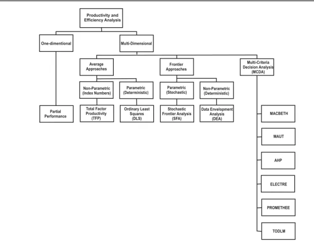
There are a large variety of benchmark methods which allows to choose the appropriate methodology to achieve the established objectives.Since airports are a multi processes system a quantitative methodologies group have been developed to assess airports productivity and efficiency performance (Liebert 2011). Really throughout the years a variety of methodologies appeared precisely to assess productivity and efficiency. Braz (2011) and von Hirschhausen and Cullmann (2005) organized these methodologies by approach type as shown in Figure 1.
One-dimensional approach, particularly partial measures, consist in dividing one output by one input, making that approach the simplest to assess productivity. However, its results must be analysed with caution because they fail to capture effects between different inputs. For this reason, to access airports performance is recommended the use of multi-dimensional approaches.
After a careful analysis of several available multi-dimensional methodsMCDA (Multi-Criteria Decision Analysis) was chosen as the most suitablefor this study. MCDA is a tool intended to help decision makers precisely to make a choice when facingmultiple and conflicting criteria situations. Indeed a MCDA problem consists in consideringdifferent choices or courses of action (Belton and Stewart 2002). MCDA methods have been developed to improve decision quality involving multiple criteria by making choices more explicit, rational and efficient (Marttunen 2010).
This methodology meets the objective to analyse airport performance considering a wide range of key performance areas and indicators that among them have different relevance. The weakness of this method lies on the fact that key performance areas and indicators relevance
assessment is based on expert’s experience and their own judgment, so results can be affected by subjective factors (Jardim 2012).
Methodology
After a careful analysis of all available MCDA tools(Braz 2011) concluded that MACBETH (Measuring Attractiveness by a Categorical Based Evaluation Technique) complied with the needed requirements for sucha research work. Also (Bana e Costa et al. 2005) underline that this multi-criteria decision analysis approach only requires qualitative judgments about value differences to help a decision maker, or a decision-advising group, to quantify relative attractiveness among several options. Measuring Attractiveness by a Categorical Based Evaluation Technique (MACBETH)
MACBETH is a decision making method that allows options evaluation in a multiple criteria scenario. MACBETH main difference among other MCDA methods is that it only needs qualitative judgements about attractiveness difference between two elements at a time in order to generate each criteria’s weights and numerical scores (Baltazar et al. 2014).
Figure 1. Quantitative Methodologies to Assess Productivity and Dfficiency. Source: Adapted from (Braz 2011; von Hirschhausen and Cullmann 2005).
When evaluator judgements are set their consistency is verified and corrections may be needed to avoid inconsistencies if they arise. Then MACBETH developsa quantitative evaluation from evaluator’s qualitative judgements. For this quantitative evaluation model a value scale is calculated for each criteria and its weights. Value scores are subsequently aggregated additively taking all the criteria into consideration to calculate the overall value scores thus reflecting their attractiveness (Gómez et al. 2007).
First, and tomake the final result more robust, it’s necessary to obtain a large data collection about the study object so a decision group can have a global view about the decisions to be taken. Next step is to create a decision tree with nodes, that is, a decision model. Nodes correspond to indicators that are going to be considered; each decision maker defines each indicator attractiveness in the tree. MACBETH have seven attractiveness difference qualitative categories: no difference, very weak, weak, moderate, strong, very strong, and extreme (Bana E Costa et al. 2012).
This model, using MACBETH methodology, values aviation managers and expert’s judgements, thus allowingto integrate their expertise and opinion in the model evaluation process, that is, in the final scores obtained.
Performance and Efficiency Support Analysis for Airport Global Benchmarking (PESA – AGB)
PESA-AGB (Performance and Efficiency Support Analysis for Airport Global Benchmarking) model was built to assess airports performance and efficiency in each KPA (Key Performance Area) and in each KPI (Key Performance Indicator). This model is based on the MACBETH mathematical foundations and it consists in a six steps organized arrangement: Structuring (Step 1); Survey (Step 2); Meeting (Step 3); Evaluation (Step 4); Classification (Step 5); and Outputs (Step 6).
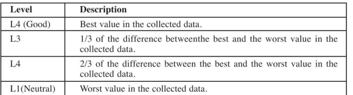
Step 1 consists in collecting airport data for each KPI. With this dataa performance descriptor with four levels(L1, L2, L3 and L4) is built for each KPIas explained in Table 1. Table 1. Performance Descriptor.
Level Description
L4 (Good) Best value in the collected data.
L3 1/3 of the difference betweenthe best and the worst value in the collected data.
L4 2/3 of the difference between the best and the worst value in the collected data.
L1(Neutral) Worst value in the collected data. Source: Own elaboration.
Step 2 and Step 3 represent collected expert’s judgments through survey and/or meetings. Using expert’s answers statistical average, a status quo scale is created.
Step 4 is a judgement matrix creation for each KPA and KPI. With all the judgments matrix created each KPA and KPI weight ponderation is determined.
Step 5 uses the performance descriptions and weight ponderation to obtain each KPA and KPI score for each option.
Step 6 produces a large variety of outputswhich allows to monitor performance over time. These outputs consist in performance profiles, sensibility analysis, options and difference profiles, and value by KPI, KPA, airports (internal benchmarking) and airport groups (external benchmarking).
Key Performance Areas (KPA’s) and Key Performance Indicators (KPI’s)
There are many different circumstances related with airport operations (aviation activities, commercial activities, location constraints, etc.) and it’s important to find different key performance areas and indicators in order to be the most accurate for the analysis (Jardim 2012). Moreover
(ACI 2012) elaborated a guide to measure airport performance which allowed a decision tree construction with six KPA’s: Core, Safety and Security, Service Quality, Productivity/Cost Efficiency, Financial/Commercial, and Environmental. Each KPA is associated with several KPI’s -a total of forty-two items as referred by(Baltazar and Silva 2016):
(i) Core - Used to characterize and categorize airports such as the number of passengers and operations. Although airports may have little control over these core indicators, especially in the short term, those are important indicators about overall airport activity, and important drivers and components of other indicators (ACI 2012). This KPA is described by five KPI’s; (ii) Safety and Security – These are critical airport
functions which sometimes overlap. Safety indicators are used to track airfield safety issues as well as safety issues involving other airport portions, including roadways and general employee safety. Security indicators may be used to track security violations, thefts and crimes, and responsiveness (ACI 2012). This KPA is described by six KPI’s;
perceive service level provided by the airport, and on service delivery objective measures (ACI 2012). This KPA is described by eight KPI’s;
(iv) Productivity/Cost Efficiency - Airports often combine productivity and cost effectiveness in a single KPA. As used by ICAO productivity refers to output to input relationship while cost effectiveness refers to the financial input or cost required to produce a non-financial output (ACI 2012). This KPA is described by nine KPI’s;
(v) Financial/Commercial – Covers a wide range of measures that analyses airport’s financial performance including airport charges, airport financial strength and sustainability, and individual commercial functions performance(ACI 2012). This KPA is described by eight KPI’s;
(vi) Environmental - Many airports have developed or are developing environmental performance indicators. These indicators are used to track an airport’s progress in minimizing its operations environmental impacts (ACI 2012). This KPA is described by six KPI’s. In this study, to search forhinterland tourism evolution it was taken into] account some socio-economic indicators presented in literature and available in INE (National Statistics Institute) which resulted in the following set (Alves 2014):
(i) Hotel Establishments - Hotels, aparthotel, guesthouses, motels, tourist villages,by square kilometre;
(ii) Accommodation Capacity –Beds available for sale in Hotel Establishments;
(iii) Bed Occupation Rate - Ratio between beds occupied and beds offered in Hotel Establishments.
These three indicators constitute our hinterland tourism KPA whichare evaluated applying the same methodology and PESA-AGB model steps.
Experts Survey and Meetings
As mentioned above to obtain KPA’s and KPI’s judgment matrix an online survey was sent to more than five hundred experts in the studied areas. The survey was applied in 2015 (Núcleo de Investigação em Transportes (NIT) 2015)and obtained a total of 81 answers. Note that PESA model doesn’t rely on the number of answers but on the quality of the answers and its relevance to each particular case under study.
Thus, the survey consisted in the following six steps: (i) Welcome message;
(ii) Experts personal information: name, email and professional expertise;
(iii) To rank KPA’s by relevance order, from 1 (least relevant) to 6 (most relevant). Different KPA’s could be assigned with the same rank;
(iv) To choose KPAfield of expertise;
(v) To rank KPI’s of the KPA selected in (iv) by relevance order, from 1 (least relevant) to 6 (most relevant). Different KPI’s could be assigned with the same rank; (vi) To fill all KPI’s judgement matrix. For each judgement matrix six questions were asked, so that: A refers to KPI best option, D refers to KPI worst option, B and C were intermediate values equally distributed between A and D. To answer these questions six semantic attractiveness difference categories wereproposed: “very weak”, “weak”, “moderate”, “strong”, “very strong” or “extreme”, so that:
a) Question 1. AD - A is more attractive than D. The difference is…?
b) Question 2. AC - A is more attractive than C. The difference is…?
c) Question 3. BD - B is more attractive than D. The difference is…?
d) Question 4. AB - A is more attractive than B. The difference is…?
e) Question 5. BC - B is more attractive than C. The difference is…?
f) Question 6. CD - C is more attractive than D. The difference is…?
With experts’ answers statistical averaging it’s possible to build three outputs that reflecteach KPA and associated KPI’s expert’s opinions.
These survey results are introduced in PESA – AGB model as inputs of step 4.
Also, meetings are a process accepted by this model to get experts opinions in assessing airports performance. These meetings consist in a key players gathering,who wish to analyse and solve an important issue related to their organization. This process is assisted by an impartial facilitator - who is a specialist in decision analysis and works as a process consultant, using a model of relevant data and judgements created on the spot to assist the group to think more clearly about the related issue (Baltazar and Silva 2016).
In this study the survey didn’t refer part of the model, more particularlyhinterland tourism KPA achievement level, subsequently weight assignment for each indicator was obtained throughout a negotiation meeting with a group of seven experts. All of them were professionals involved in tourism areas. Authors played the facilitator role,allowing experts different opinions, assessingtrade-offs, and agreeing on final weights and attractiveness differences.
Case Study
This case study is an example to understand how airports performance and their impacts can be studied with a
complete PESA – AGB model and its hinterland relation. Although, this case study only presents Faro’s airport KPA Core final score, the model will also provide all KPA’s and KPI’s scores, as well an overall Faro’s airport performance score.
From all Portuguese airports, Faro airport (in the South) was chosen for this study due to LCC’s largest market share recorded with 13 LCC’s representing 83% of all aircraft movements(Costa and Almeida 2015).
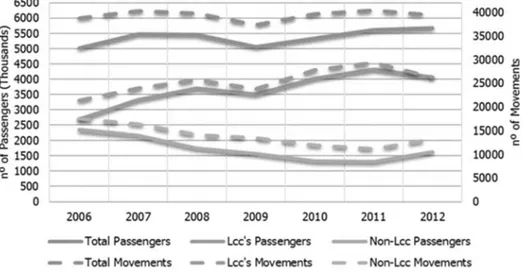
Before applying PESA – AGB model, LLC’s movements and passengersnumber evolution in Faro airport is analysed (Figure 2). Collected data corresponds to a seven years period, from 2006 to 2012 (ANA - Aeroportos De Portugal 2006, 2016, Instituto Nacional de Aviação Civil 2008, 2012), due to the lack of more recent years data availability from Portuguese airports. These two parameters analysis are important sinceboth passengers and movements are key performance indicators in Core KPA, and the objective is to understand the correlation magnitude/importance between this Core and HinterlandTourism KPA.
Figure 2. Faro’s Airport Passengers and Movements Evolution (2006 -2012). Source: OwnelaborationbasedonANA - Aeroportos De
Portugal 2006, 2016/ Instituto Nacional de Aviação Civil 2008, 2012
An interesting observation is that LCC’s movementsevolution is the most significant factor influencing passenger numbers and aircraft movements data in Core KPA. It’s possible to observe that passengers or movements (orange line) seems to be defining Faro’s airport
overall passengers and movements numbers (blue line). Non LCC’s movements (grey line) exhibits a slow, but constant, reduction,except for 2011-2012 period.
Faro’s airport overall movementshas been increasing from 2006, with the 2008-2009 and 2011-2012 time periods exception, also identified by (EUROCONTROL 2014).
Table 2. Faro’s Airport Core and Hinterland Tourism Indicators Weights. Weights
Faro’s Airport Core Key Passengers Number 25,71%
Performance Indicators Origin and Destination Passengers 20,00%
Aircraft Movements 22,86%
Freight and Mail Loaded / Unloaded 17,14%
Destinations (Nonstop) 14,29%
Faro’s Hinterland Tourism Hotel Establishments 30,00%
Key Performance Indicators Accommodation Capacity 30,00%
Bed Occupation Rate 40,00%
inTable 2.
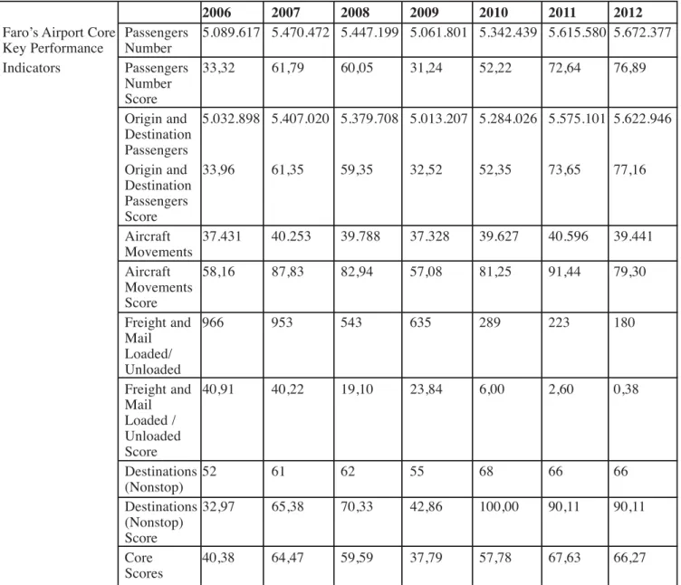
Expert’s judgements on each KPI relevance shows that, in Core KPA, the most relevant KPI’s are passengers number and aircraft movements, totalizing almost 50% of the KPA weight. Furthermore, Bed Occupation Rate KPI was consideredHinterland’s Tourism KPA most relevantindicator, representing 40% of its total weight. Table 3 shows Faro’s airport Core KPA and KPI’s values and scores. Hinterland Tourism indicators data wascollected from (INE 2013) and are presented in Table 4along with respective scores.
After analysing Faro’s airport movements evolution, PESA-AGB model, explained in section 4.2, was applied to determine each KPA and KPI score, focused on Core KPA score. PESA-AGB methodology also was applied to determine Hinterland Tourism KPA and its KPI’s scores. Duringthe experts meeting, as explained in section 4.4, weights were attributed to Hotel Establishments, Accommodation Capacity and Bed Occupation Rate which reflect its relevance in Hinterland Tourism KPA. Core’s key performance indicators weights were determined by expert’s judgementsobtained through the survey, alsoas described in section 4.4. The obtained weights are presented
Table 3. Faro’s Airport Core KPA and KPI’s Respective Values and Scores.
2006 2007 2008 2009 2010 2011 2012
Faro’s Airport Core Passengers 5.089.617 5.470.472 5.447.199 5.061.801 5.342.439 5.615.580 5.672.377 Key Performance Number
Indicators Passengers 33,32 61,79 60,05 31,24 52,22 72,64 76,89 Number Score Origin and 5.032.898 5.407.020 5.379.708 5.013.207 5.284.026 5.575.101 5.622.946 Destination Passengers Origin and 33,96 61,35 59,35 32,52 52,35 73,65 77,16 Destination Passengers Score Aircraft 37.431 40.253 39.788 37.328 39.627 40.596 39.441 Movements Aircraft 58,16 87,83 82,94 57,08 81,25 91,44 79,30 Movements Score Freight and 966 953 543 635 289 223 180 Mail Loaded/ Unloaded Freight and 40,91 40,22 19,10 23,84 6,00 2,60 0,38 Mail Loaded / Unloaded Score Destinations 52 61 62 55 68 66 66 (Nonstop) Destinations 32,97 65,38 70,33 42,86 100,00 90,11 90,11 (Nonstop) Score Core 40,38 64,47 59,59 37,79 57,78 67,63 66,27 Scores
Source: Ownelaborationbased on ANA - Aeroportos De Portugal 2006, 2016/Instituto Nacional de Aviação Civil 2008, 2012
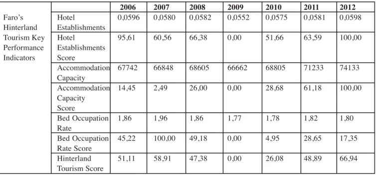
Table 4. Faro’s Hinterland Tourism KPA and KPI’s Respective Values and Scores.
2006 2007 2008 2009 2010 2011 2012
Faro’s Hotel 0,0596 0,0580 0,0582 0,0552 0,0575 0,0581 0,0598
Hinterland Establishments
Tourism Key Hotel 95,61 60,56 66,38 0,00 51,66 63,59 100,00
Performance Establishments Indicators Score Accommodation 67742 66848 68605 66662 68805 71233 74133 Capacity Accommodation 14,45 2,49 26,00 0,00 28,68 61,18 100,00 Capacity Score Bed Occupation 1,86 1,96 1,86 1,77 1,78 1,82 1,80 Rate Bed Occupation 45,22 100,00 49,18 0,00 4,95 28,65 17,35 Rate Score Hinterland 51,11 58,91 47,38 0,00 26,08 48,89 66,94 Tourism Score
Source: Own elaboration based onINE 2013 All key performance indicators from Faro’s Hinterland Tourism KPA seem to evidence the same evolution pattern
Figure 3 Depicts Table 3 and Table 4 Collected Data.
Figure 3. Faro’s Airport Core KPA Vs Faro’s Hinterland Tourism KPA Scores. as LCC’s passengers and movements, showing a decrease in 2008-2009time period.
Source: Own elaboration based on ANA - Aeroportos De Portugal 2006, 2016/ Instituto Nacional de Aviação Civil 2008, 2012
Figure 3 identifies a possible correlation between LCC’s operation, airport Core performance and Hinterland Tourism areas, since both KPA’s show are markable performance decrease in the same time period as LCC’s passengers and movements, that is, 2008-2009.
Next step isa possible correlation identification and related
magnitudeevaluation between Faro’s airport Core area and its Hinterland. A linear regression method was applied, using SPPS Statistical software, to determine correlation coefficients, namelyPearson Correlation Coefficient2,
Kendall Rank Correlation Coefficient 3and Spearman’s
Rank Correlation Coefficient45.
Table 5 and Table 6 presentthe statistic results based onTable 3 and Table 4variables.
Table 5. Descriptive Statistics
Mean Standard Deviation Sample size (N)
Faro’sAirport Core (KPA) 56,27 12,27 7
Hotel Establishments (KPI) 62,54 33,03 7
Hinterland Tourism (KPA) 42,76 22,66 7
Bed Occupation Rate (KPI) 35,05 34,18 7
Accommodation Capacity (KPI) 33,26 35,86 7
Source: Own elaboration
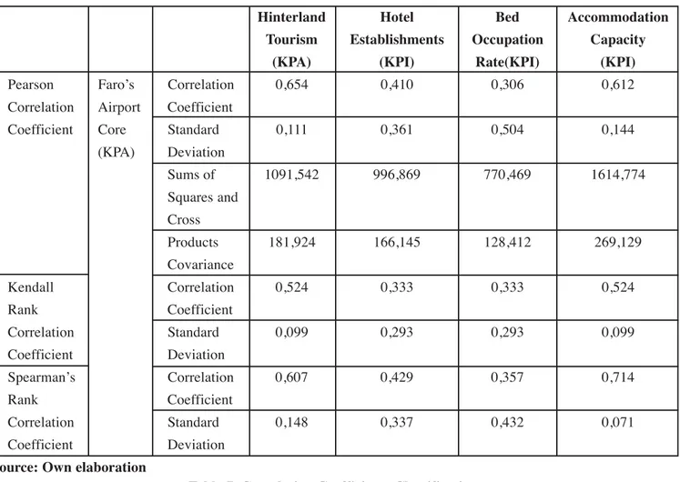
Hinterland Tourism and Faro’s airport Core KPA’s correlation is the most important parameter to analyse in this study, and from Table 6 we obtain values as 0,654,
0,524, and 0,607 determined by Pearson Correlation Coefficient, Kendall Rank Correlation Coefficient and Spearman’s Rank Correlation Coefficient, respectively. Table 6. Correlation Coefficients.
Hinterland Hotel Bed Accommodation
Tourism Establishments Occupation Capacity
(KPA) (KPI) Rate(KPI) (KPI)
Pearson Faro’s Correlation 0,654 0,410 0,306 0,612
Correlation Airport Coefficient
Coefficient Core Standard 0,111 0,361 0,504 0,144
(KPA) Deviation Sums of 1091,542 996,869 770,469 1614,774 Squares and Cross Products 181,924 166,145 128,412 269,129 Covariance Kendall Correlation 0,524 0,333 0,333 0,524 Rank Coefficient Correlation Standard 0,099 0,293 0,293 0,099 Coefficient Deviation Spearman’s Correlation 0,607 0,429 0,357 0,714 Rank Coefficient Correlation Standard 0,148 0,337 0,432 0,071 Coefficient Deviation
Source: Own elaboration
Table 7. Correlation Coefficients Classification. [0,9;1] Very strong positive correlation. [0,7;0,9] Strong positive correlation. [0,5;0,7] Moderate positive correlation. [0,3;0,5] Low positive correlation. [0;0,3] Negligible correlation. Source: Adapted from(Taylor 1990).
Regarding both Table 6 - correlation coefficients between Faro’s airport Core and Hinterland Tourism KPI’s,and Table 7 - correlation coefficients classification, it’s possible to observethat Hotel Establishments and Bed Occupation Rate indicators exhibit a low positive correlation (coefficients between 0.3 and 0.5). Nevertheless,Accommodation Capacity indicator exhibits a moderate positive correlation (coefficient between 0.5 and 0.7) with Faro’s airport Corebased on Pearson and Kendall Rank Correlation Coefficients; but based on Spearman’s Rank Correlation Coefficient, accommodation capacity exhibits a strong positive correlation with Faro’s airport Core, that is, 0,714. Conclusion and Future Work
PESA – AGB model, as well as Hinterland Tourism KPA model, show similar performance evolution as of LCC’s movements, having the same2008 to 2009 drop.
The case study evidences a possible correlation between an airport’s Hinterland Tourism evolution and its Core KPA changes. Moreover, it evidencesa moderate correlation between these two factors. However, the sample size is very small to support the observed correlations.
It’s possible to conclude that Accommodation Capacity KPI exhibits a more similar correlation with airport’s Core KPA than the others. This means that although expert’s judgments classified Accommodation Capacity as 30% of the Hinterland Tourism KPA weight, nevertheless it’sthe onethat expressesa better correlation.
The three HinterlandTourism indicators identified and analysedshow a similar trend throughout the studied timespan, but it’s interesting to observe that
Accommodation Capacity variation seems to have one-year delay from Bed OccupationRate variation; which may lead to the conclusion thatbeds occupation, decrease or increase,can influencetheAccommodation Capacity, decrease or increase number,in the next year.
This studywas usedto testhow some traditional statistical methodsmay be used to determinecorrelationbetween airport specific variables and the related hinterland. Nevertheless, the use of a MCDA methodology to analyse correlations between LCC movements, airport’s performance and its hinterland still require a deeperbibliographic revision and research work.
It’s important to note that the lack of available data limited the study time period too, which resulted in small samples size.
To determine LCC’s operationimpact on hinterland (and vice versa) it’s suggested to add more research work as follows:
(a) to investigate KPA and KPI where LCC’s have a greater impact on airport performance;
(b) to extend this evaluation to a wider hinterland socio-economic indicators number, including indicators outside the tourism area;
(c) to evaluate a new hinterland model, with new inputs from (b), using PESA-AGB model methodology, and so determiningairport’s performance and hinterland KPI’s correlation;
(d) to extend this study to other airports as the referred PESA models allow an easy replicability.
References
1. Abdi, H. (2007), The Kendall Rank Correlation Coefficient, Encyclopedia of Measurement and Statistics, 508–510, Available at https://www.utdallas.edu/~herve/Abdi-KendallCorrelation2007-pretty.pdf, Accessed on 1 February 2008.
2. ACI (2006), Airport Benchmarking To Maximise Efficiency, World Economics, July. 3. ACI (2011), ACI Statistics Manual: A practical guide addressing best practices 2011. 4. ACI (2012), Guide to Airport performance measures.
5. Almeida, C. (2011), Low Cost Airlines, Airports and Tourism. The Case of Faro Airport, 51st ERSA Congress.
6. Alves, P. (2014), Determination and Evaluation of an Airport Catchment Area: a Portuguese Case Study. Universidade da Beira Interior.
7. Alves, P., Baltazar, M. E., Silva, J., Garra, J., and Vaz, M. (2013), The Impact of Hinterland over The Global Efficiency of Airports, in 19th Portuguese Association for Regional Development (APDR) Congress, 1–17.
8. ANA (2006), Annual report and accounts 2006.
9. ANA (2016), RouteLAB, Available at http://routelab.ana.pt/, Accessed on 1st October 2016.
10. Baltazar, M. E. and Silva, J. (2016), Global Decision Support for Airport Performance and Efficiency Assessment, in 20th
ATRS World Conference.
11. Baltazar, M. E., Jardim, J., Alves, P.and Silva, J. (2014), Air Transport Performance and Efficiency: MCDA vs. DEA Approaches,
12. Bana e Costa, C., De Corte, J.M., Vansnick (2012), Macbeth, International Journal of Information Technology and Decision
Making, 11(2), 359–387, Doi:10.1142/S0219622012400068.
13. Bana e Costa, C., De Corte, J.M., Vansnick, J.C., Costa, J., Chagas, M.P., Corrêa, E.C., João, I., Lopes, F., Lourenço, J. and Sánchez-López, R. (2005), M-MACBETH User’s Guide (Version 2.4.0), Available at http://www.m-macbeth.com/help/pdf/M-MACBETH%202.4.0%20Users%20Guide.pdf, Accessed on 2nd March 2005.
14. Belton, V., and Stewart, T. J. (2002), Multiple Criteria Decision Analysis: An Integrated Approach. Doi:10.1007/978-1-4615-1495-4.
15. Braz, J. (2011), O MacBeth como ferramenta MCDA para o Benchmarking de Aeroportos. Universidade da Beira Interior. 16. Costa, V., and Almeida, C. (2015), Low-Cost Carriers, Local Economy and Tourism Development At Four Portuguese Airports.
A Model of Cost-Benefit Analysis, Journal of Spatial and Organizational Dynamics, III(4), 245–261.
17. EUROCONTROL (2014), EUROCONTROL Seven-Year Forecast February 2014 - 7-year IFR Flight Movements and Service
Units Forecast/ : 2014-2020, Available athttps://www.eurocontrol.int/sites/default/files/content/documents/official-documents/
forecasts/seven-year-flights-service-units-forecast-2014-2020-feb2014.pdf, Accessed on 3rd April 2014.
18. Figueiredo, V. (2010), Companhias Aéreas de Baixo Custo e Desenvolvimento do Turismo: Percepções dos Stakeholders da
Região Centro. Universidade de Aveiro. Available athttp://hdl.handle.net/10773/1774, Accessed on 4th May 2010.
19. Fröhlich, K., andNiemeier, H.-M. (2011), The importance of spatial economics for assessing airport competition, Journal of
Air Transport Management, 17(1), 44–48. Doi:10.1016/j.jairtraman.2010.10.010
20. Gautheir, T. D. (2001), Detecting Trends Using Spearman’s Rank Correlation Coefficient, Environmental Forensics, 2(4), 359–362. Doi:10.1080/713848278
21. Gómez, C., Ladevesa, J., Prieto, L., Redondo, R., Gibert, K., andValls, A. (2007), Use and Evaluation Of M-MACBETH. 22. Graham, A. (2008), Managing Airports - An International Perspective, Elsevier [Third Edition].
23. INE (2013), Dados Estatísticos. Available athttps://www.ine.pt, Accessed on 16th October 2013. 24. Instituto Nacional de Aviação Civil (2008), Anuário da Aviação Civil 2003 - 2007.
25. Instituto Nacional de Aviação Civil (2012), Impacto das Transportadoras de Baixo Custo no Transporte Aéreo Nacional (1995
- 2011), Lisbon.
26. Jardim, J. (2012), Airports Efficiency Evaluation Based on MCDA and DEA Multidimensional Tools. Universidade da Beira Interior.
27. Kasarda, J. D. (2001), Logistics and the rise of Aerotropolis, Real Estate Issues, (winter 2000/2001), 43–48.
28. Liebert, V. P. (2011), Airport Benchmarking An Efficiency Analysis of European Airports from an Economic and Managerial Perspective. Available athttps://opus.jacobs-university.de/frontdoor/index/index/docId/127, Accessed on 5th June 2011. 29. Lieshout, R. (2012), Measuring the size of an airport’s catchment area, Journal of Transport Geography, 25, 27–34. Doi:10.1016/
j.jtrangeo.2012.07.004.
30. Lopes, D. R. (2008), Airport performance and Benchmarking: um experimento brasileiro, VII Simpósio de Transporte Aéreo
-SITRAER, 7, 293–304.
31. Marcucci, E., andGatta, V. (2011), Regional airport choice: Consumer behaviour and policy implications, Journal of Transport
Geography, 19(1), 70–84. doi:10.1016/j.jtrangeo.2009.10.001
32. Marttunen, M. (2010), Description of Multi-Criteria Decision Analysis (MCDA). Available athttp://environment.sal.aalto.fi/ MCDA/, Accessed on 10th September 2016.
33. Núcleo de InvestigaçãoemTransportes (NIT) (2015), Judgement Analysis of Airport Performance Areas and Indicators Survey. Available at http://goo.gl/forms/UFxeB2M663, Accessed on 1st February 2017.
34. Rodgers, J. L., andNicewander, W. A. (1988), Thirteen Ways to Look at the Correlation Coefficient, The American Statistician, 42(1), 59. Doi:10.2307/2685263.
35. Rosa, T., Baltazar, M. E., and Silva, J. (2015), MCDA Modelling of Airport Impacts due to LCC ’ s Operation, in International
Conference on Engineering of University of Beira Interior - Engineering for Society.
catchment area analysis using a GIS approach, Journal of Air Transport Management, 34(0), 12–16. Doi:http://dx.doi.org/ 10.1016/j.jairtraman.2013.07.004.
37. Taylor, R. (1990), Interpretation of the Correlation Coefficient: A Basic Review, Journal of Diagnostic Medical Sonography, 6(1), 35–39. Doi:10.1177/87564793900060 0106
38. Thelle, M., Pedersen, T., andHarhoff, F. (2012), Airport Competition in Europe, Copenhagen Economics.
39. Vaz, M., Silva, J., Baltazar, M. E., and Marques, T. (2013), Regional Airports and Regional Development: Two Portuguese Case Studies, in 19th Portuguese Association for Regional Development (APDR) Congress.
40. vonHirschhausen, C., andCullmann, A. (2005), Questions to airport benchmakers - some theoretical and pratical aspects learned from benchmarking other sectors’, in German Aviation Research Society Conference on Benchmarking and Airport
Competition. Vienna.
41. Wilhelm, J. (2016), What is the minimum sample size to run Pearsons R?, Available at https://www.researchgate.net/post/ What_is_the_minimum_sample_size_to_run_Pearsons_R, Accessed on 21st February 2017.
Endnotes
1. Corresponding author. Tel.: +351926355453; E-mail address: tiagorosa.nit@ubi.pt
2. Pearson Correlation Coefficient - Measure of linear dependence (correlation) between two variables. It is determined
dividing the covariance of two variables by the product of their standard deviations (Rodgers and Nicewander 1988).
3. Kendall Rank Correlation Coefficient - Non-parametric hypothesis test for statistical dependence based on the tau coefficient.
It is a measure of rank correlation: the similarity of the orderings of the data when ranked by each of the quantities (Abdi 2007)
4. Spearman’s Rank Correlation Coefficient - Non-parametric measure of rank correlation. Spearman correlation between
two variables is equal to the Pearson correlation between the rank values of those two variables. However, Pearson’s correlation assesses linear relationships, while Spearman’s correlation assesses monotonic relationships (linear or not) (Gautheir 2001). 5. Our sample size is n=7. However, “[T]echnically one can calculate a correlation coefficient from n=2. There is no problem
having a small sample size. The only difficult thing is to see or recognize possibly relevant deviations from these assumptions with small samples. But this does not invalidate the test, because the test remains valid under these assumptions” (Whillelm 2016).