doi: 10.5540/tema.2018.019.03.0449
Higher Order Markov Chain Model for
Synthetic Generation of Daily Streamflows
A.G.C. PEREIRA1, F.A.S. SOUSA2, B.B. ANDRADE3and V.S.M. CAMPOS4
Received on November 10, 2016 / Accepted on April 19, 2018
ABSTRACT.The aim of this study is to further investigate the two-state Markov chain model for synthetic generation of daily streamflows. The model presented in [4] to determine the state of the stream and later studied in [2] and [3] is based on two Markov chains, both of order one. In some areas of Hydrology, where Markov chains of order one have been successfully used to model events such as daily rainfall, researchers are concerned about the optimal order of the Markov chain [10]. In this paper, an answer to a similar concern about the model developed in [4] is given using the Bayesian Information Criterion (BIC) to establish the order of the Markov chain which best fits the data. The methodology is applied to daily flow series from seven Brazilian sites. It is seen that the data generated using the optimal order are closer to the real data than when compared to the model proposed in [4] with the exception of two sites, which exhibit the shortest time series and are located in the driest regions.
Keywords: Bayesian Information Criterion, Hydrology, Stochastic Processes.
1 INTRODUCTION
In water resources, one of the first daily flow models was Svanidse’s approach [17] in which the process was modeled based on the definition of a fragment. The fragment is a set of annual daily flows sequences obtained by dividing the daily flows of the considered year by the mean annual flow of the same year. The procedure can be described by (a) the generation of the mean annual flow value; (b) random drawing with replacement of one element of the fragment set; and (c) multiplication of every member of the fragment by the mean annual flow value. Besides the over-reliance on the mean flow, Svanidse’s model has the additional shortcoming of assuming
*Corresponding author: Viviane Simioli Medeiros Campos – E-mail: [email protected]
1Departamento de Matem´atica, UFRN - Universidade Federal do Rio Grande do Norte, Avenida Salgado Filho, 3000, 59.078-970, Natal, RN, Brazil. E-mail: [email protected]
2Unidade Acadˆemica de Ciˆencias Atmosf´ericas, UFCG - Universidade Federal de Campina Grande, Rua Aprigio Veloso, 882, 58.429-900, Campina Grande, Para´ıba, Brazil. E-mail: [email protected]
3Departamento de Estat´ıstica, UnB - Universidade de Bras´ılia, Campus Darcy Ribeiro, 79.910-900, Bras´ılia, Distrito Federal, Brazil. E-mail: [email protected]
independence between the mean annual flow and properties of daily flows within the annual period.
Soon after the proposal of Svanidse’s model, autoregressive models were used for simulation of daily flows [6, 13]. In [6], the mean monthly flows are generated first and, in a next step, they are dismembered into daily values using a second-order autoregressive model, AR(2). In [13], the AR(2) model is directly used to simulate daily flow. In both cases, statistical characteristics of the AR(2) process are estimated over time. These AR(2) models cannot reproduce recessions because of the underlying white noise processes.
Later, a model to generate daily streamflow based on linear interpolation of five-day average flows using statistical modeling for the non-deterministic component of the daily time series was proposed by [9]. However, the model masks short-term fluctuations, an important feature in daily streamflow. Non-parametric techniques were used in [12]. The advantage is that non-parametric methods do not require distributional specifications needed by parametric methods. Generated streamflow series using this technique may retain the marginal and joint density structure of the observed hydrologic series including nonlinearity and state dependence. Seasonality in the daily flow process was modeled by [18] by assuming a periodic structure, within an annual cycle, of the daily mean and variance. At the same time, he assumed that the system’s response function was invariant accross the annual cycle, stating that this assumption was often made but only quoting a past writing [20] in which there are no grounds for such assumption.
One of the objectives in stochastic hydrology is to generate synthetic streamflow sequences that are statistically similar to observed data. Statistical similarity implies that the generated sequences have statistical and dependence properties similar to those of the historical record. In fact, autoregressive moving average models, ARMA(p,q), together with the Fractional Gaussian Noise (FGN) model and variations dominate streamflow generation [19]. Several of these models have been applied to daily streamflow generation. However, ARMA(p,q)recessions, which are sums of negative exponential functions, could not account for the prominent features of daily streamflow. Even when seasonality is considered (SARIMA), such models cannot capture the peculiarities of daily flow data.
Markov chains have also been used as an important tool in the studies of hydrometeorological variables at a daily time interval [14]. Some seminal works include [15] and extensions [4, 5]. These extended models consist of four steps: (i) determination of the days in which flow occurs, (ii) determination of the days in which a flow increment occurs, (iii) determination of the flow increment, and (iv) calculation of the flow decrement on days when the flow is reduced. In [5], the first two steps are modeled by a three-state Markov chain and in [4] these steps are modeled by two two-state Markov chains. The applicability of both techniques is showed in [2] and their performances can be seen in [3] where the conclusion is that both alternatives are capable of simulating the state of the stream.
or-der for stremflows. Our paper is concerned with the estimation of the optimal oror-der of Markov chains used in [4] for generation of daily streamflows. In particular, the Bayesian Information Criteria (BIC) is used to determine the order that better fits a given set of data. We employ this technique to data from seven Brazilian sites. After estimating the optimal order, we fit the corre-sponding Markov chain and use it for synthetic generation of daily streamflow, thereby providing basic hydrologic data for integrated water resources management in the sites considered.
2 METHODOLOGY
The basic model employed here is based on the following steps described in [4] and [2]: for each month we determine (i) days in which flow occurs, (ii) days in which a flow increment occurs, (iii) the flow increment/decrement. The two first steps are modeled by two Markov chains. At step (i), a 1 - 0 Markov chain of order one is used to assign 1 for the occurrence of flow and 0 for the non-occurrence of flow:
"
P11 P10
P01 P00 #
, (2.1)
wherePi jdenotes the probability that the system makes a (one-step) transition to state jgiven that it is at state i and the resulting 2×2 matrix represents the transition matrix of the two-state Markov chain modeling flow occurrence. Once a day with flow has been determined, step (ii) uses another two-state Markov chain of order one to choose between an increment (R) or a decrement (F) of flow for that day:
"
PRR PRF PFR PFF
#
, (2.2)
whereRcorresponds to a day with a flow increment (rise) andFcorresponds to a day with a flow decrement (fall).
In this paper, we modify the basic model described above by letting the order of the Markov chains used in steps (i) and (ii) be determined by the value of the BIC, estimated from the data.
2.1 Determination of the order of the Markov chains based on information criteria
Akaike’s Information Criterion (AIC) is the standard metric for model comparison in several areas of data analysis, notably in time series and stochastic processes [7]. However, it is not consistent to estimate the order of a Markov chain based on the asymptotic distribution of the resulting estimator [11]. Looking for estimators that have better properties, [11] has suggested the Bayesian Information Criterion (BIC) [16] as an alternative to the AIC. The orderβis estimated by ˆβ which is the value that minimizes the BIC across the models being entertained:
Consider a Markov chain of orderβ withNstates such thatni1,i2,...,iβ is the number of times that (i1,i2, ...,iβ)appears in a sample of sizen. Then
BIC(β) =−2 N
∑
i1,i2,...,iβ+1=1ni1,i2,...,iβ+1log
ni1,i2,...,iβ+1
ni1,i2,...,iβ
!
+γ(β)log(n), (2.4)
whereγ(β) =Nβ(N−1)is the number of free parameters under the hypothesis that the order isβ. Strong consistency of the BIC-derived estimator has been proved and extended for cases where finiteness of the order is not assumed [8].
Here, for each month, the BIC is used to estimate the order of the chain that best models flow/no flow and of the chain for increment/decrement. Thus, if the BIC of the raise/fall chain of a given month indicates that the order is zero, the values of the increment or decrement of the samples are obtained independently using the rate of climbs as success probability. If the order is one, the transition matrices flow/no flow and increment/decrement reduce to (2.1) and (2.2) respectively.
When the order of the Markov chain is two, the current state receives two pieces of information, the first information at timet and the second information at timet+1 (for rises and falls, for example, the possible states are:RR,RF,FR, andFF). Thus, the first pair of information refers to timest andt+1 and the second pair to timest+1,t+2. Generally speaking, in a Markov chain{xt}t∈Nof order two, the transition matrix is given by
P(AB,CD) =P(xt+2=D,xt+1=C|xt+1=B,xt=A), (2.5)
whereA,B,C,Dare states of the chain and its transition matrix is estimated by
ˆ
P(AB,CD) =
nABD
nAB•, ifnAB•6=0, B=C, 0, ifnAB•6=0, B6=C,
δAB(CD), ifnAB•=0,
wherenABD is the number ofABDtransitions that appear in the sample,nAB•is the number of
ABT triples whereT is any of the possible states of the chain, andδAB(CD)is the Kronecker delta, which is equal to 1 whenAB=CD(A=CandB=D) and zero otherwise.
2.2 Flow increment and flow decrement
The flow increment is the difference between successive daily flows when the flow of the current day is greater than the flow of the previous day. Based on data, and following [4, 2, 1], the flow increment is modeled with a two-parameter gamma distribution with density function
f(x) =λ
αxα−1e−λx
Γ(α) , x>0, (2.6)
whereαandλ are the shape and scale parameters, respectively, andΓdenotes the gamma func-tion. The expected value E[X] and variance Var[X] of the two-parameter gamma distribution are
E(X) =α
λ and Var(X) =
α
λ2. (2.7)
Given daily observed historical series, the expectation and the variance above are replaced by the corresponding monthly sample statistics, so the shape (α) and scale (λ) parameters of the distribution are estimated for each month,
ˆ
α=
¯ x S
2
and λˆ = x¯ S2,
where ¯xandSare the sample mean and standard deviation, respectively, for a given month.
The total number of parameters required for this step of the model is, thus, 24 for each of the seven sites analyzed in Section 3 below.
In order to determine the flow decrement, which occurs when the flow of the current day is less than the flow of the previous day, the data are divided in two sets:
• days in which the decrement happened when the flow of the previous day is greater than the monthly mean flow.
• days in which the decrement happened when the flow of the previous day is less than the monthly mean flow.
The values of the first set are used to estimate the parameterb1, the flow decrement rate in one day. Once again, following [4, 2], the parameterb1models the flow decrement when the flow of the previous day (Qt−1) is greater than the monthly mean flow by means of
Qt=Qt−1e−b1. (2.8)
In a similar way, the values of the second set are used to estimate the parameterb2, that models the flow decrement when the flow of the previous day (Qt−1) is less than the monthly mean flow by the equation:
Qt=Qt−1e−b2. (2.9)
𝑡←𝑡+1
Start
Has flow occured?
𝑥!
𝑄!!!
=0
𝑄!!!=𝑄!+ increment Has an increment
occured?
𝑄!!!=𝑄!𝑒! !!
𝑄!!!=𝑄!𝑒! !
!
𝑄!>monthly flow average? yes
yes
yes
no no
no
= 0
Figure 1: Flow chart.
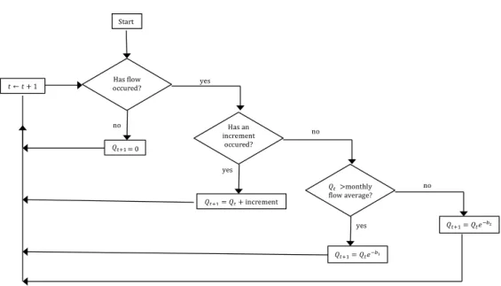
2.3 The flow chart
Using the values of all parameters previously calculated and beginning with a flow value that is randomly generated from the set of all values observed in the first day of the historical data (usually Jan 1st) the generated streamflow is obtained as given in the flow chart in Figure 1.
When a new month is reached, parameters are automatically updated to the corresponding month, and the process continues. As used in Aksoy’s model, this process is repeated 10 times. Each period should have a length of 10 times the number of years of data used, that is, if the size of the data sample is 10 years, each realization should be run for 100 years.
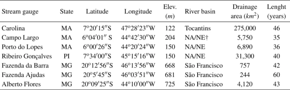
3 HISTORICAL DATA USED
Table 1: Basic information on gauging stations used in the analysis. † NA/NE refers to North Atlantic/Northeast basin.
Stream gauge State Latitude Longitude Elev. River basin Drainage Lenght
(m) area (km2) (years)
Carolina MA 7o20′15′′S 47o28′23′′W 122 Tocantins 275,000 46
Campo Largo MA 6o04′01′′S 44o42′30′′W 204 NA/NE† 5,750 35
Porto do Lopes MA 6o00′26′′S 44o20′24′′W 150 NA/NE 6,890 36
Ribeiro Gonc¸alves PI 7o34′00′′S 45o15′16′′W 150 NA/NE 31,300 40
Fazenda da Barra MG 20o12′56′′S 46o13′56′′W 668 S˜ao Francisco 757 42
Fazenda Ajudas MG 20o5′45′′S 46o03′51′′W 681 S˜ao Francisco 244 60
Alberto Flores MG 20o09′25′′S 44o10′00′′W 725 S˜ao Francisco 4,120 43
4 RESULTS
4.1 Illustration with the Carolina river data
The Carolina River is used next to illustrate the procedure proposed here to estimate the order of the Markov chain that modeled the increment/decrement flow. In the sequel, the estimated order given by the BIC analysis for each river is presented as well as the parameters of the functions that modeled the flow increment and the flow decrement.
Using eq. (2.4) with data from the Carolina River, the values of the BIC for each month are shown in Table 2.
Table 2: BIC values for rise/fall - Carolina River Data; minimum BIC in bold.
Month β
0 1 2 3 4 5
January 1919 1353 1317 1299 1294 1352
February 1677 1169 1144 1103 1114 1168
March 1857 1289 1267 1242 1253 1308
April 1711 1257 1211 1184 1181 1236
May 1163 872 847 812 823 878
June 909 679 658 648 671 729
July 945 658 640 645 646 697
August 1239 842 821 799 821 889
September 1723 1186 1151 1130 1127 1191
October 1876 1462 1429 1407 1422 1467
November 1789 1392 1354 1323 1316 1372
December 1912 1387 1345 1308 1312 1361
Table 3: Optimal order of rise/fall chains for each month - Carolina River.
Jan Fev Mar Apr May Jun Jul Aug Sep Oct Nov Dec
β 4 3 3 4 3 3 2 3 4 3 4 3
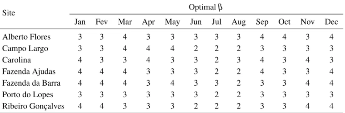
4.2 Summary of results from all rivers
Implementing the same scheme illustrated above for the Carolina River to the other six sites yields the results in Table 4. Note that the chosen order was always greater than one.
Table 4: Optimal order of rise/fall chains, for each month, obtained from analyzing the BIC values for the seven sites used in the analysis.
Site Optimalβ
Jan Fev Mar Apr May Jun Jul Aug Sep Oct Nov Dec
Alberto Flores 3 3 4 3 3 3 3 3 4 4 3 4
Campo Largo 3 3 4 4 4 2 2 2 3 3 3 3
Carolina 4 3 3 4 3 3 2 3 4 3 4 3
Fazenda Ajudas 4 4 4 3 3 3 2 2 4 3 3 4
Fazenda da Barra 4 4 4 3 4 3 3 2 3 3 4 4
Porto do Lopes 3 3 3 3 3 3 2 2 3 3 3 3
Ribeiro Gonc¸alves 4 4 3 3 3 2 2 2 3 3 4 4
The flow generation scheme proposed in [4], using Markov chains of order one, reproduced the main features of daily flows quite successfully.
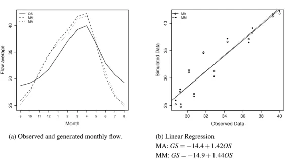
Next, we compare the results from the scheme proposed here (MM), using Markov chains with estimated order (via BIC), with the results obtained from the model presented in [4] (MA) for each of the seven stream gauges. Tables 5–11 show streamflow values generated by MM and those generated by MA. In the last line of each table, the distance between the observed data and each generated data are displayed. The metric used to calculate such distance is
kOS−GSk=
s 12
∑
i=1[OS(i)−GS(i)]2,
whereiindexes month,OSrepresents the observed streamflow andGSrepresents the generated streamflows. The metrickOS−GSkfavors MM over MA for five of the sites. The exceptions are Campo Largo and Porto Lopes for whichGSMA<GSMM.
month. In most cases, both schemes tend to overestimate the monthly flow withGScurves almost entirely above theOScurve. This cannot be due to faulty choice of the chain order since both models differ in that respect (MA fixed at order one and MM based on the BIC). We believe that the flow increment/decrement scheme described in Section 2.2, which is used in both models, is the source of the problem.
Table 5: Observed (OS) and generated (GS) streamflows for the two models considered – Carolina site.
OS GS
MM MA
January 6168 7012 7075 February 7306 7716 7686 March 7313 7786 7866 April 6108 6571 6518
May 3593 4275 4248
June 2213 2913 2964 July 1674 2496 2594 August 1357 2575 2548 September 1256 2912 2920 October 1575 3144 3189 November 2495 3713 3684 December 4433 5592 5545 kOS−GSk 3530 3567
Table 6: Observed (OS) and generated (GS) streamflows for the two models considered – Campo Largo site.
OS GS
MM MA
January 34.33 37.19 36.61 February 37.03 39.14 38.31 March 39.27 41.73 41.28 April 40.00 42.28 41.82 May 36.63 36.50 37.12 June 32.89 30.29 31.25 July 30.73 26.66 27.10 August 29.29 25.25 24.75 September 28.73 25.92 25.21 October 29.21 27.95 27.54 November 30.18 31.04 31.38 December 31.75 34.48 34.68 kOS−GSk 9.01 8.72
1000 2000 3000 4000 5000 6000 7000 8000 Month Flo w a ver age
9 10 11 12 1 2 3 4 5 6 7 8
OS MM MA
(a) Observed and generated monthly flow.
● ● ● ● ● ● ● ● ● ● ● ●
2000 3000 4000 5000 6000 7000
3000 4000 5000 6000 7000 8000 Observed Data Sim ulated Data ● ● ● ● ● ● ● ● ● ● ● ● ● ● MA MM
(b) Linear Regression
MA:GS=1457+0.865OS
MM:GS=1439+0.867OS
25 30 35 40 Month Flo w a ver age
9 10 11 12 1 2 3 4 5 6 7 8
OS MM MA
(a) Observed and generated monthly flow.
● ● ● ● ● ● ● ● ● ● ● ●
30 32 34 36 38 40
25 30 35 40 Observed Data Sim ulated Data ● ● ● ● ● ● ● ● ● ● ● ● ● ● MA MM
(b) Linear Regression
MA:GS=−14.4+1.42OS
MM:GS=−14.9+1.44OS
Figure 3: Comparison of monthly observed and generated flows – Campo Largo.
Table 7: Observed (OS) and generated (GS) streamflows for the two models considered – Porto do Lopes site.
OS GS
MM MA
January 35.46 39.06 37.78
February 38.78 41.66 40.85
March 41.09 44.76 43.69
April 42.31 44.07 43.24
May 38.02 37.95 38.04
June 33.12 32.44 32.76
July 30.74 28.93 28.79
August 29.33 27.15 26.60
September 28.77 28.05 27.56
October 29.23 30.60 29.86
November 30.40 33.19 32.40
December 32.51 35.52 34.70
kOS−GSk 8.08 6.26
Table 8: Observed (OS) and generated (GS) streamflows for the two models considered – Ribeiro Gonc¸alves site.
OS GS
MM MA
January 294.7 320.4 310.9
February 326.5 320.2 328.7
March 316.3 329.9 338.6
April 277.3 303.4 310.5
May 207.0 236.6 250.3
June 170.0 177.1 184.8
July 155.0 134.5 137.1
August 143.4 113.0 110.0
September 139.1 140.8 145.3
October 161.3 200.0 205.9
November 209.3 250.5 254.9
December 257.4 293.4 294.5
30 35 40 45 Month Flo w a ver age
9 10 11 12 1 2 3 4 5 6 7 8
OS MM MA
(a) Observed and generated monthly flow.
● ● ● ● ● ● ● ● ● ● ● ●
30 32 34 36 38 40 42
30 35 40 Observed Data Sim ulated Data ● ● ● ● ● ● ● ● ● ● ● ● ● MA MM
(b) Linear Regression
MA:GS=−6.15+1.20OS
MM:GS=−6.34+1.22OS
Figure 4: Comparison of monthly observed and generated flows – Porto Lopes.
150 200 250 300 Month Flo w a ver age
9 10 11 12 1 2 3 4 5 6 7 8
OS MM MA
(a) Observed and generated monthly flow.
● ● ● ● ● ● ● ● ● ● ● ●
150 200 250 300
150 200 250 300 Observed Data Sim ulated Data ● ● ● ● ● ● ● ● ● ● ● ● ● ● MA MM
(b) Linear Regression
MA:GS=−4.32+1.10OS
MM:GS=−8.05+1.01OS
Table 9: Observed (OS) and generated (GS) streamflows for the two models considered – Fazenda da Barra site.
OS GS
MM MA
January 52.20 58.18 59.06
February 47.25 57.70 56.31
March 38.06 45.91 47.28
April 24.10 34.21 32.57
May 13.75 31.31 33.16
June 10.28 26.10 29.44
July 8.36 25.34 31.89
August 7.15 28.06 33.56
September 7.11 36.04 34.42
October 10.83 22.71 25.14
November 21.11 26.95 27.55
December 41.17 45.45 45.67
kOS−GSk 51.21 57.38
Table 10: Observed (OS) and generated (GS) streamflows for the two models considered – Fazenda Ajudas site.
OS GS
MM MA
January 11.47 12.96 13.17
February 9.90 10.71 10.58
March 8.81 10.02 10.11
April 6.24 7.40 7.85
May 3.92 6.80 7.13
June 2.95 5.64 6.09
July 2.38 4.78 4.66
August 1.89 4.66 4.83
September 1.82 5.22 5.34
October 2.13 4.82 5.07
November 3.61 6.00 5.8
December 7.27 9.68 9.78
kOS−GSk 8.06 8.60
10 20 30 40 50 60 Month Flo w a ver age
9 10 11 12 1 2 3 4 5 6 7 8
OS MM MA
(a) Observed and generated monthly flow.
● ● ● ● ● ● ● ● ● ● ● ●
10 20 30 40 50
25 30 35 40 45 50 55 60 Observed Data Sim ulated Data ● ● ● ● ● ● ● ● ● ● ● ● ● MA MM
(b) Linear Regression
MA:GS=23.9+0.60OS
MM:GS=20.5+0.68OS
2
4
6
8
10
12
Month
Flo
w a
ver
age
9 10 11 12 1 2 3 4 5 6 7 8
OS MM MA
(a) Observed and generated monthly flow.
●
●
●
●
●
●
● ● ● ●
●
●
2 4 6 8 10
6
8
10
12
Observed Data
Sim
ulated Data
●
●
●
●
●
●
● ● ● ●
●
● ●
● MA MM
(b) Linear Regression
MA:GS=3.40+0.79OS
MM:GS=3.22+0.80OS
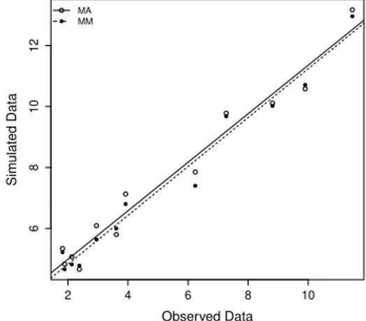
Figure 7: Comparison of monthly observed and generated flows – Fazenda Ajuda.
Table 11: Observed (OS) and generated (GS) streamflows for the two models considered – Alberto Flores site.
OS GS
MM MA
January 123.71 134.33 132.85
February 96.96 118.78 114.46
March 81.48 96.38 101.16
April 55.26 80.54 83.40
May 41.62 82.72 82.98
June 35.29 77.84 79.09
July 30.33 76.17 78.15
August 26.46 86.63 84.63
September 27.71 74.69 75.52
October 35.31 55.98 59.77
November 57.87 70.961 72.45
December 96.37 110.61 115.8
40
60
80
100
120
Month
Flo
w a
ver
age
9 10 11 12 1 2 3 4 5 6 7 8
OS MM MA
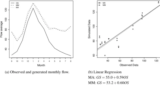
(a) Observed and generated monthly flow.
●
●
●
● ● ● ● ●
●
● ●
●
40 60 80 100 120
60
80
100
120
Observed Data
Sim
ulated Data
●
●
●
● ●
● ● ●
●
●
● ●
● MA MM
(b) Linear Regression
MA:GS=55.0+0.59OS
MM:GS=53.2+0.60OS
Figure 8: Comparison of monthly observed and generated flows – Alberto Flores.
5 CONCLUSION
The use of a variable order for the Markov chains modeling streamflow data is a viable and simple feature, which can be incorporated into any modeling scheme in stochastic hydrology based on Markov chains. Here, we have done so by incorporating higher order chains into a scheme previously used to model streamflow data [4, 2, 3], which is based on Markov chains of order one. Such scheme was used to describe the occurrence of daily streamflow followed by stochastic modeling (via Gamma distribution) of flow increment and a simple exponential fit to model flow decrement. Based on the distance between the observed and generated (monthly) average flows, the results using higher order chains were better than using order one, with the exception of two studied cases, which have the shortest time series and are located in the driest region of Maranh˜ao state. The proposed criterion for choosing the order has been the BIC.
ACKNOWLEDGMENT
We would like to thank the reviewers who have improved this work and also to thank the CNPq for the financial support.
´e dada, usando o crit´erio de informac¸˜ao de Bayes para estabelecer a ordem de cadeia de Markov que melhor se encaixa nos dados. A metodologia ´e aplicada a uma s´erie de fluxos di´arios de sete rios brasileiros. Observa-se que os dados gerados usando a ordem estimada de cada cadeia s˜ao mais pr´oximos dos dados reais do que o modelo proposto em [4], com excec¸˜ao de dois locais que tˆem as menores s´eries temporais e est˜ao localizados nas regi˜oes mais secas.
Palavras-chave:Hidrologia, processos estoc´asticos, crit´erio de informac¸˜ao bayesiano.
REFERENCES
[1] H. Aksoy. Use of gamma distribution in hydrological analysis. Turkish Journal Engineering
Environmental Sciences,24(2000), 419–428.
[2] H. Aksoy. Markov chain-based modeling techniques for stochastic generation of daily intermittent
streamflows.Advances in Water Resources,26(2003), 663–671.
[3] H. Aksoy. Using Markov chains for non-perennial daily streamflow data generation. Journal of
Applied Statistics,31(2004), 1083–1094.
[4] H. Aksoy & M. Bayazit. A Daily Intermittent streamflow simulator.Turkish Journal Engineering
Environmental Sciences,24(2000), 265–276.
[5] H. Aksoy & M. Bayazit. A model for daily flows of intermittent streams.Hydrological Processes,14
(2000), 1725–1744.
[6] L.R. Beard. Simulation of daily streamflow. Technical report, US Army Corps of Engineers, Institute for Water Resources, Hydrologic Engineering Center, Fort Collins (1967).
[7] G.E.P. Box & G. Jenkins. “Time Series Analysis: Forecasting and Control”. Holden-Day, San Francisco (1976).
[8] I. Csisz´ar & P. Shields. The consistency of the BIC Markov order estimator.Annals of Statistics,6
(2000), 1601–1619.
[9] N.M.D. Green. A synthetic model for daily streamflow.Journal of Hydrology,20(1973), 351–564.
[10] O.D. Jimoh & P. Webster. The optimum order of a Markov chain model for daily rainfall in Nigeria.
Journal of Hydrology,185(1996), 45–69.
[11] R.W. Katz. One some criteria for estimating the order of Markov chain.Technometrics,23(1981),
1243–249.
[12] J. Prairie, B. Rajagopalan, U. Lall & T. Fulp. A stochastic nonparametric technique for
space-time disaggregation of streamflows. Water Resources Research, 43 (2007), 1–10. doi:10.1029/
2005WR004721.
[13] R.G. Quimpo. Stochastic analysis of daily river flows.Journal of the Hydraulics Division ASCE,94
(1968), 43–58.
[15] D.M. Sargent. A simplified model for the generation of daily streamflows.Hydrological Sciences Bulletin,24(1979), 509–527.
[16] G. Schwarz. Estimating the dimension of a model.Annals of Statistics,6(1978), 461–464.
[17] G.G. Svanidse. “Principles of estimating river flow regulation by the Monte Carlo method”. Metsniereba Press, Tbilisi, USSR (1964).
[18] G. Weiss. Shot noise models for the generation of synthetic streamflow data. Water Resources
Research,13(1977), 101–108.
[19] S.J. Yakowitz. A nonparametric Markov model for daily river flow.Water Resources Research,15
(1979), 1035–1043.
[20] G.K. Young & W.C. Pisano. Operational hydrology using residuals.Journal of the Hydraulics Division