Structural dynamic analysis for time response of bars and
trusses using the generalized finite element method
Abstract
The Generalized Finite Element Method (GFEM) can be viewed as an extension of the Finite Element Method (FEM) where the approximation space is enriched by shape func-tions appropriately chosen. Many applicafunc-tions of the GFEM can be found in literature, mostly when some information about the solution is known a priori. This paper presents the application of the GFEM to the problem of structural dynamic analysis of bars subject to axial displacements and trusses for the evaluation of the time response of the struc-ture. Since the analytical solution of this problem is com-posed, in most cases, of a trigonometric series, the enrich-ment used in this paper is based on sine and cosine func-tions. Modal Superposition and the Newmark Method are used for the time integration procedure. Five examples are studied and the analytical solution is presented for two of them. The results are compared to the ones obtained with the FEM using linear elements and a Hierarchical Finite El-ement Method (HFEM) using higher order elEl-ements. Keywords
dynamic analysis, structural dynamics, time response, hi-erarchical finite element method, generalized finite element method, partition of unity method.
Andr´e Jacomel Torii∗ and
Roberto Dalledone Machado
Graduate Program in Numerical Methods in Engineering (PPGMNE), Federal University of Paran´a (UFPR), Brazil.
Received 09 Apr 2012; In revised form 08 May 2012
∗Author email: [email protected] 1
1 INTRODUCTION
2
There is an increasingly effort among the engineering community for the design of structures
3
that allow the efficient use of resources and construction procedures. In this context, the design
4
of efficient structures can only be accomplished when the structural behavior is known in
5
details. The dynamic behavior of structures requires particular attention since most methods
6
available for this kind of analysis need significant computational effort. Consequently, the
7
development of more accurate methods can reduce the amount of computational effort needed
8
in order to solve a given problem for the same accuracy, allowing the engineer to study a larger
9
range of structural solutions and thus conceive better structures.
10
Most practical problems from structural dynamic analysis are solved using numerical
meth-11
ods. When the time response of the structure is sought the problem can be decomposed in
two parts. The first regards the approximation of time variations, that can be made by
13
some time integration scheme such as the Newmark Method and the Modal Superposition
14
Method[7, 15, 42]. The second is the solution of the resulting boundary value problem for each
15
discrete time step. Some methods commonly used for solving boundary value problems are:
16
the Finite Difference Method[27], the Boundary Element Method[2], the Meshfree Methods[29]
17
and the Finite Element Method (FEM)[7, 23, 42].
18
The application of several methods for the solution of structural dynamics problems have
19
already been proposed[11, 14, 28, 30], being one of the most common approaches the use of the
20
FEM together with direct integration methods[7, 23, 42]. However, several authors observed
21
that low order polynomial finite elements may give poor results for structural dynamic analysis
22
and thus proposed some kind of improved approach[3, 6, 10, 18, 19, 22, 26, 34, 39–41].
23
Most improved versions of the FEM for structural dynamics involve the enrichment of the
24
approximation space by some set of functions. In this context, two general trends can be
ob-25
served in literature: the enrichment of the approximation space by complete polynomial bases
26
or trigonometric bases that resemble the polynomial ones [6, 10, 22, 34]; and the enrichment of
27
the approximation space by trigonometric bases that reproduce some fundamental vibration
28
mode of the structure[18, 19, 26, 40, 41].
29
In the last decades, the development of the Partition of Unity Finite Element Method
30
(PUFEM)[5, 31] and its variants, the Generalized Finite Element Method (GFEM)[4, 37] and
31
the Extended Finite Element Method (XFEM) [1, 16], allowed new possibilities to the problem
32
of structural dynamics[3, 9, 20, 35].
33
The works by [9] and [20] applied the PUFEM to evaluate the response spectrum of plates,
34
obtaining better results than traditional approaches. The application of the GFEM to the
35
problem of modal analysis of bars and trusses was discussed in details by [3]. The paper by
36
[35] appears to be the only one to apply the concepts of the PUFEM to evaluate the time
37
response of structures using time integration procedures. In the work by [35] the method is
38
used to model discontinuities inside a given structure without the need for a finite element
39
mesh that fits the geometry of the domain. However, in[35] the method is not used to enrich
40
the approximation space of the FEM, but only to reduce the need for using very small finite
41
elements due to mesh geometry constraints.
42
The work by [3] showed that an approach based on the GFEM is able to obtain very
43
accurate results for the problem of modal analysis. This is possible since the enrichment shape
44
functions can be built as to resemble the fundamental vibration modes of the structure. Since
45
Modal Superposition is based on the fundamental vibration modes of the structure [7, 15, 42],
46
it is expected that the approach proposed by[3] is also able to give accurate results for the
47
time response analysis.
48
In this paper the approach proposed by [3] for modal analysis of bars subject to axial
49
displacements and trusses is applied to structural dynamic analysis in order to obtain the
50
time response of the structure. For the time integration procedure the Modal Superposition
51
approach and the Newmark Method (with α = 0.5 and δ = 0.25) are used [7, 15, 42]. The
52
efficiency of the proposed approach is compared with the polynomial Hierarchical Finite
ment Method (HFEM) as described by[36] and the standard linear FEM [7, 23] by means of
54
five examples. High resolution versions of the figures containing the time responses presented
55
in this paper are also available online as supplementary files.
56
The importance of studying the problem in the one dimensional framework is that the shape
57
functions used for two dimensional problems can be obtained by taking products of the one
58
dimensional shape functions[13, 23, 36]. However, it is easier to obtain analytical solutions for
59
one dimensional problems, what allows a rigorous comparison between the accuracy obtained
60
by the approximate methods. The extension of the approach proposed here for two dimensional
61
problems remains as subject of future works.
62
2 HIERARCHICAL FINITE ELEMENT METHOD
63
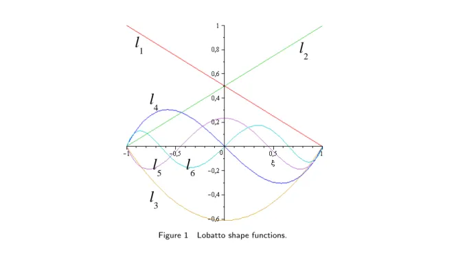
The HFEM for the problem being addressed can be formulated using Lobatto polynomials as
64
described by[36]. Some Lobatto polynomials for a finite element with coordinates ξ = [-1,1]
65
are
66
l1(ξ)=
1−ξ
2 , (1)
67
l2(ξ)=
1+ξ
2 , (2)
68
l3(ξ)=
1 2
√
3 2(ξ
2
−1), (3)
69
l4(ξ)=
1 2
√
5 2(ξ
2
−1)ξ, (4)
70
l5(ξ)=
1 8
√
7 2(ξ
2
−1) (5ξ2−1) (5)
and
71
l6(ξ)=
1 8
√
9 2(ξ
2
−1)(7ξ2−3)ξ, (6)
that are presented in Fig. 1. The mass and stiffness matrices can be obtained using the shape
72
functions from Eqs. (1)–(6) by the standard procedure used for the FEM[7, 23, 42]. Here, the
73
consistent mass matrix is used.
74
By assuming only the shape functions from Eq. (1) and Eq. (2) one obtains the lagrangian
75
linear finite element[7, 23, 42]. However, the extra shape functions that allow higher order
76
approximations are all zero at the nodes of the finite element. This ensures that the standard
77
procedures used for the linear FEM still hold for the HFEM[36]. Imposition of boundary
78
conditions and manipulation of nodal quantities remain the same as used for the FEM. Note
79
that if more than one shape function is not zero in a given node of the finite element, special
80
techniques must be used to impose the boundary conditions of the problem, such as the
81
Lagrange Multiplier Method or some Penalty Method[12, 13]. For this reason most hierarchical
82
approaches introduce extra shape functions that are null at the nodes of the finite element.
l
6
l
1
l
2
l
3
l
4
l
5
Figure 1 Lobatto shape functions.
The main characteristic of the HFEM is that when the order of the approximation is
84
increased the shape functions already in use remain unchanged. The traditional FEM with
85
shape functions given by Lagrange polynomials do not share this property, making the use of
86
higher order approximations very difficult[36].
87
3 GENERALIZED FINITE ELEMENT METHOD
88
In the standard lagrangian FEM, the displacements inside a given finite element are
approxi-89
mated by[7, 8, 23, 42]
90
uh= n ∑ i=1
uiNi(ξ), (7)
where ui are nodal degrees of freedom, Ni are the polynomial shape functions, ξ is the local
91
coordinate system of the element andn is the number of shape functions.
92
In the context of the GFEM, the approximation given by Eq. (7) can be enriched by
93
considering an approximate solution given by
94
uh= n ∑ i=1
uiNi(ξ)+ m ∑ j=1
cjφj(ξ), (8)
where φj are enrichment functions and cj are the associated degrees of freedom. Here the
95
enrichment functions φj are obtained using the PUFEM[31] as described by [3, 39].
96
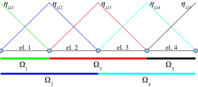
In the PUFEM the shape functions are given by the multiplication of a Partition of Unity
97
(PU) by basis functions appropriately chosen. The PU used here is the one defined by the shape
98
functions obtained for the lagrangian linear finite element, since the sum of these functions
99
results in one[8, 23]. This PU is as shown in Fig. 2 and respects the conditions described by
100
[31].
In Fig. 2, the finite elements are tagged el. 1, el. 2, etc, while the functions that composed
102
the PU are tagged ηΩ1, ηΩ2, etc. Each function ηΩjis defined in a subdomain Ωi that is 103
defined by the union of two neighbor finite elements, except for Ω1and Ω5. In the context of 104
the PUFEM the subdomains Ωi are called covers or patches. In general, each finite element
105
is defined in the intersection between two patches. More details on the PUFEM can be found
106
in[5, 31].
107
ηΩ1
Ω1
Ω2
Ω3
Ω4 Ω5
ηΩ2 ηΩ3 ηΩ4 ηΩ5
el. 1 el. 2 el. 3 el. 4
Figure 2 A PU given by linear shape functions of the lagrangian FEM.
Inside a finite element with local coordinates ξ = [-1,1] the PU can be written as
108
η1(ξ)=
1−ξ
2 (9)
and
109
η2(ξ)=
1+ξ
2 , (10)
that are shown in Fig. 3.
110
η
1η
2The basis functions used here are the ones proposed by [3]. Inside a finite element with
111
local coordinatesξ = [-1,1] these functions can be written as
112
v4j−3=sin(βj(
ξ+1)
2 ), (11)
113
v4j−2=cos(βj(
ξ+1)
2 )−1, (12)
114
v4j−1=sin(βj(
ξ−1)
2 ) (13)
and
115
v4j =cos(βj(
ξ−1)
2 )−1, (14)
whereβj is a parameter that allows the modification of the shape functions. The basis functions
116
and the PU forβj =π are shown in Fig. 4.
117
η1 η2
v
1
v2 v
3
v
4
Figure 4 Basis functions and PU inside a finite element forβj=π.
The basis functions from Eqs. (11)-(14) were chosen as trigonometric functions since the
118
analytical solution of most problems from dynamic analysis of bars are composed of
trigono-119
metric terms[15, 25, 32]. However, the basis functions from Eqs. (11)-(14) were carefully build
120
as to result in shape functions that are zero at the nodes of the finite element, as discussed
121
later.
122
In the context of modal analysis, an optimal value for βj can be estimated in order to
123
obtain best results for the approximation of a given fundamental vibration mode. An efficient
iterative scheme for evaluating the optimal value for βj was proposed by[3] and leads to very
125
accurate results.
126
The shape functions for a finite element can be obtained by the multiplication of the PU by
127
the basis functions, following the procedure described by[3]. The contribution from the patch
128
to the left of the finite element is given by the multiplication of v4j−3 and v4j−2 by η1. The 129
contribution from the patch to the right is given by the multiplication ofv4j−1 and v4j by η2. 130
The resulting PUFEM shape functions are:
131
φ4j−3=
1−ξ
2 [sin(βj
(ξ+1)
2 )], (15)
132
φ4j−2=
1−ξ
2 [cos(βj
(ξ+1)
2 )−1], (16)
133
φ4j−1=
1+ξ
2 [sin(βj
(ξ−1)
2 )] (17)
and
134
φ4j =
1+ξ
2 [cos(βj
(ξ−1)
2 )−1]. (18)
The nodal shape functions can be taken as η1 and η2 itself, that are the Lagrange linear 135
polynomials. The approximation space is then given by
136
VGF EM =VF EM⋃VP U F EM, (19)
whereVGF EM is the approximation space of the GFEM used here,VF EM is the approximation
137
space from the FEM using linear finite elements and VP U F EM is the approximation space
138
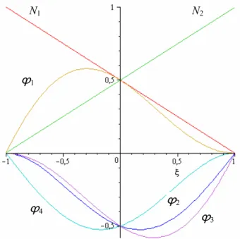
obtained by the PUFEM and defined by the shape functions from Eqs. (15)-(18). The resulting
139
shape functions forβj=πare shown in Fig. 5. The mass and stiffness matrices can be obtained
140
by the standard procedure used for the FEM [7, 23, 42]. Here, the consistent mass matrix is
141
used.
142
By modifying the value ofβj one is able to adapt the shape functions for different cases[3].
143
Besides, several sets of enrichment function from Eqs. (15)-(18) can be considered by assuming
144
different values ofβj. In order to build a finite element with 10 shape functions, for example,
145
one can consider β1 = π and β2 = 2π and include 8 enrichment functions. Including more 146
enrichment functions can be made without changing the enrichment functions already used
147
and thus the GFEM proposed here is a hierarchical method. This simplifies computational
148
implementation and allows the use of higher order approximations.
149
As can be seen from Fig. 5, the enrichment functions are zero at the nodes of the finite
150
element. It can be demonstrated that this is true for any value of βj. Consequently, the
151
implementation of boundary conditions and manipulation of nodal quantities is the same as
152
for the standard FEM and do not require special techniques. However, in order to ensure this
153
property the basis functions were carefully designed. The use of other sets of trigonometric
154
functions may not maintain this property.
ϕ
ϕ ϕ
ϕ
Figure 5 Shape functions inside a finite element forβj=π.
Here, both the stiffness and mass matrices remain constant during the entire dynamic
anal-156
ysis. The same occurs for the shape functions. Consequently, the mass and stiffness matrices
157
are evaluated only once, at the beginning of the dynamic analysis, and remain unchanged for
158
the entire analysis. Once the stiffness and mass matrices are evaluated the dynamic analysis
159
is made in the same way as occurs for the standard lagrangian FEM and the HFEM. In this
160
work we have not checked the influence of time dependent shape functions, mass matrices and
161
stiffness matrices. An approach where the shape functions are updated iteratively in order to
162
comply with wave propagation angles was presented by[9], for a two dimensional problem.
163
The stiffness and mass matrices were obtained using analytical integration, by using
soft-164
ware for symbolic manipulation. These matrices were obtained for a finite element with
ar-165
bitrary values for the element length, elastic modulus, density, cross sectional area and the
166
parameter β. The stiffness and mass matrices in closed form were then incorporated into the
167
computational routine responsible for the dynamic analysis. It is important to point out that
168
the analytical integration of the mass and stiffness matrices is not possible in most GFEM
169
applications. In fact, numerical integration in the context of the GFEM is a delicate matter,
170
since the shape functions may not be polynomials and then numerical integration may not
171
be exact. A more detailed discussion on numerical integration for the GFEM is presented by
172
[4]and [17].
173
The nodal degrees of freedom of the FEM, the HFEM and the GFEM (as presented here)
174
are the same and are related to nodal displacements. These degrees of freedom are ruled by
175
the linear lagrangian shape functions. However, the extra degrees of freedom of the HFEM
176
and the GFEM (given by the Lobatto polynomials in the case of the HFEM and by the
PUFEM shape functions in the case of the GFEM) have no direct physical meaning. These
178
extra degrees of freedom affect the displacements inside the domain of the finite element, but
179
are not particularly related to a single point of the domain, as occurs for the nodal degrees
180
of freedom. For this reason, these extra degrees of freedom are also called field degrees of
181
freedom.
182
Here, the field degrees of freedom are all zero at the nodes of the finite elements and thus
183
nodal displacements can be obtained directly, by taking the value of the associated nodal
184
degree of freedom. If one needs to evaluate displacements inside some finite element, then it
185
is necessary to take into account the contribution of each shape function of the finite element.
186
In this context, the way the degrees of freedom are defined for the HFEM and the GFEM do
187
not affect the comparison of the results. In all three methods, nodal displacements can be
188
read directly while displacements inside the finite elements can be evaluated by summing the
189
contribution of all the shape functions, as occurs in the standard FEM.
190
4 TRUSS STRUCTURES
191
In order to obtain the equilibrium equations for a truss finite element, that can be oriented
192
in an arbitrary direction in space, it is necessary to apply some coordinate transformation
193
rule[33].
194
For a linear finite element of a planar truss the following coordinate transformation hold
195
[ u′1
u′
2 ]
=[ cosθ sinθ 0 0 0 0 cosθ sinθ ]
⎡⎢ ⎢⎢ ⎢⎢ ⎢⎢ ⎣ u1 v1 u2 v2 ⎤⎥ ⎥⎥ ⎥⎥ ⎥⎥ ⎦ , (20)
where u’ are the nodal displacements in local coordinates, u and v are the horizontal and
196
vertical nodal displacements in global coordinates andθ is the inclination of the bar.
197
The coordinate transformation for the HFEM and the GFEM follows the reasoning used
198
by[41] for the Composite Element Method. Since the enrichment functions are zero at the
199
nodes of the element, the coordinate transformation is given by
200 ⎡⎢ ⎢⎢ ⎢⎢ ⎢⎢ ⎢⎢ ⎢⎣ u′ 1 u′ 2 c′ 1 ⋮ c′ n ⎤⎥ ⎥⎥ ⎥⎥ ⎥⎥ ⎥⎥ ⎥⎦ = ⎡⎢ ⎢⎢ ⎢⎢ ⎢⎢ ⎢⎢ ⎢⎣
cosθ sinθ 0 0 0 ⋯ 0
0 0 cosθ sinθ 0 ⋯ 0
0 0 0 0 1 ⋯ 0
⋮ ⋮ ⋮ ⋮ ⋮ ⋱
0 0 0 0 0 1
⎤⎥ ⎥⎥ ⎥⎥ ⎥⎥ ⎥⎥ ⎥⎦ ⎡⎢ ⎢⎢ ⎢⎢ ⎢⎢ ⎢⎢ ⎢⎢ ⎢⎢ ⎢⎢ ⎣ u1 v1 u2 v2 c1 ⋮ cn ⎤⎥ ⎥⎥ ⎥⎥ ⎥⎥ ⎥⎥ ⎥⎥ ⎥⎥ ⎥⎥ ⎦ , (21)
wherec’ are enrichment degrees of freedom in local coordinates andcare enrichment degrees of
201
freedom in global coordinates. That is, the enrichment degrees of freedom in local coordinates
202
are the same as the enrichment degrees of freedom in global coordinates.
5 ERROR EVALUATION
204
The error between the analytical solution u(x,t) and the approximate solution uh(x,t) for a
205
given position inside the bar x = x0in the time interval [ti,tf] can be defined as 206
e=∫ tf
ti
∣u(x0, t)−uh(x0, t)∣dt. (22)
In order to evaluate the error inside the entire bar one can integrate Eq. (22) along its length.
207
However, this procedure is not used in this paper because of the computational difficulties
208
involved in the evaluation of this integral.
209
Evaluating the error by using Eq. (22) may not be efficient in practice since the approximate
210
solution is generally known only at discrete time steps. However, an approximation for Eq.
211
(22) can be written as
212
e≈ nt
∑ i=1
∆t∣u(i)−u(i)
h ∣, (23)
wherent is the number of time steps used, ∆t is the time step used to obtain the approximate
213
solution, u(i) is the analytical solution at time step (i) and u
h(i) is the approximate solution
214
at time step (i).
215
Error evaluation according to Eq. (23) is illustrated in Fig. 6. The integral from Eq. (22)
216
in a given time interval is approximated by the product between ∆t and ∆u(i). Equation (23) 217
can be evaluated efficiently since it only deals with discrete values in time. More details on
218
error evaluation for the time response are presented by[39].
219
∆t
u
(i)u
h (i)
∆u
(i)t
(i)t
(i-1)t
u
6 NUMERICAL RESULTS
220
6.1 Bar subject to initial displacements
221
The first example is that of a bar fixed at both ends and subject to initial displacements as
222
shown in Fig. 7. The properties of the material were chosen to give the wave velocity equal
223
toc=√E/ρ = 1m/s and the bar length is equal to 1m. The initial displacement field is zero
224
at both ends, has a maximum value umax equal to 0.25m at the middle of the bar and has a
225
triangular shape. This initial displacement can be obtained by applying a unitary load at the
226
middle of the bar. Finally, there is no force acting on the bar and the initial velocities are null.
227
Initial displacements
u
max
Figure 7 Bar subject to initial displacements.
This problem can be stated as[38]
228
∂2u ∂x2 =
∂2u
∂t2 ∀x∈[0,1] (24) 229
⎧⎪⎪⎪⎪ ⎪⎪ ⎨⎪⎪⎪ ⎪⎪⎪⎩
u(x=0, t)=u(x=1, t)=0
u(x<0.5, t=0)=x
2
u(x≥0.5, t=0)=1−x
2
∂u(x,t=0)
∂t =0
, (25)
that is a wave propagation problem with wave velocity c = 1m/s. The analytical solution
230
can be found by separation of variables and by representing the initial conditions by a Fourier
231
series as described by [25].
232
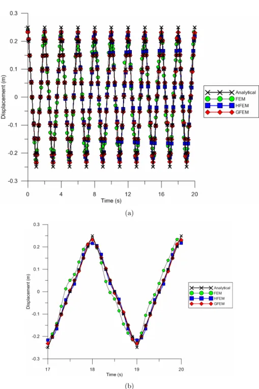
This example is first studied using Modal Superposition for a time interval of 20s and using
233
11 degrees of freedom. The resulting equations from Modal Superposition are solved using the
234
Newmark method (with α = 0.5 and δ = 0.25) for a time step equal to 2.5x10⁻³
s. For the
235
FEM the mesh is composed of 10 linear finite elements. For the HFEM the mesh is composed
236
of two finite elements of order 5, by assuming 6 polynomial shape functions. For the GFEM
237
the mesh is composed of two finite elements with 4 enrichment functions as given by Eqs.
238
(15)-(18), by assumingβ1 = 3π/2. The analytical and the approximate solutions atx = 0.5m 239
are presented in Fig. 8, considering 5 modes in Modal Superposition.
240
The errors for different numbers of modes included in the Modal Superposition analysis
241
are presented in Table 1. The errors obtained by considering only the first mode are presented
(a)
(b)
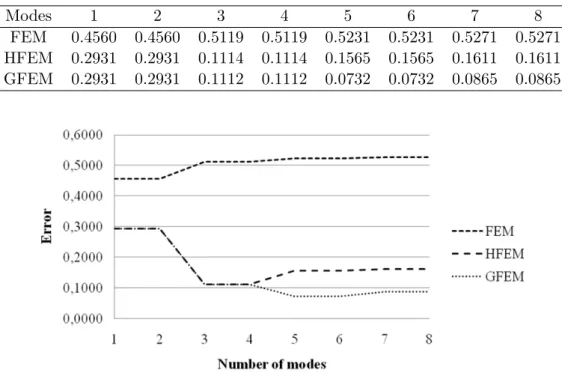
Table 1 Errors obtained with 11 degrees of freedom for different numbers of modes considered in Modal Superposition.
Modes 1 2 3 4 5 6 7 8
FEM 0.4560 0.4560 0.5119 0.5119 0.5231 0.5231 0.5271 0.5271 HFEM 0.2931 0.2931 0.1114 0.1114 0.1565 0.1565 0.1611 0.1611 GFEM 0.2931 0.2931 0.1112 0.1112 0.0732 0.0732 0.0865 0.0865
Figure 9 Errors obtained with 11 degrees of freedom for different numbers of modes considered in Modal Superposition.
in the first column, the errors obtained by considering the first two modes are presented in the
243
second columns and so on. The errors from Table 1 are also presented in Fig. 9.
244
It can be seen that the best results were not obtained by considering every fundamental
245
vibration mode of the structure. This is a general trend when dealing with Modal Superposition
246
because the higher vibrations modes of the structure may be poorly approximated by the
247
FEM[13]. Consequently, including the higher vibrations modes in Modal Superposition may
248
reduce the accuracy of the approximate solution.
249
From Table 1 and Fig. 9 it can be seen that the best results were obtained with the GFEM
250
when considering 5 or 6 modes. The best results for the HFEM were obtained when 3 or 4
251
modes were considered. The results obtained with the FEM are very poor in comparison to
252
the ones obtained with both the HFEM and the GFEM. This behavior is confirmed by the
253
displacements presented in Fig. 8.
254
From Fig. 9 another interesting conclusion can be drawn. The inclusion of the fifth mode
255
improved the solution given by the GFEM, but worsened the solution given by the HFEM.
256
This seems to indicate that the higher modes are better approximate by the GFEM in this
257
case.
258
The same problem was also solved using 19 degrees of freedom. The mesh used for the
259
FEM is composed of 18 linear finite elements. The mesh used for the HFEM is composed
260
of 2 finite elements of order 9, by assuming 10 polynomial shape functions. For the GFEM
the mesh is composed of two finite elements with 8 enrichment functions as given by Eqs.
262
(15)-(18), by assuming β1 = 3π/2 and β2 = 3π. The errors for these cases are presented in 263
Table 2 and Fig. 10.
264
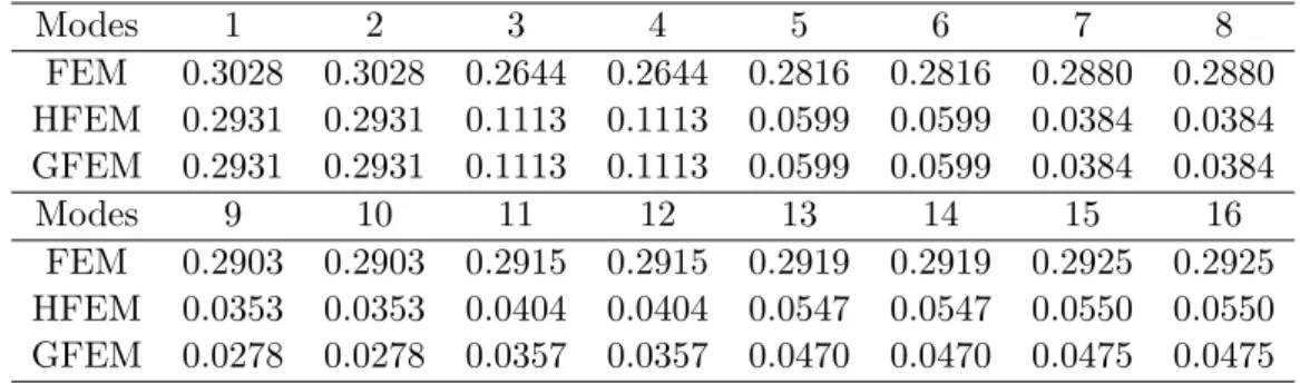
Table 2 Errors obtained with 19 degrees of freedom for different numbers of modes considered in Modal Superposition.
Modes 1 2 3 4 5 6 7 8
FEM 0.3028 0.3028 0.2644 0.2644 0.2816 0.2816 0.2880 0.2880 HFEM 0.2931 0.2931 0.1113 0.1113 0.0599 0.0599 0.0384 0.0384 GFEM 0.2931 0.2931 0.1113 0.1113 0.0599 0.0599 0.0384 0.0384
Modes 9 10 11 12 13 14 15 16
FEM 0.2903 0.2903 0.2915 0.2915 0.2919 0.2919 0.2925 0.2925 HFEM 0.0353 0.0353 0.0404 0.0404 0.0547 0.0547 0.0550 0.0550 GFEM 0.0278 0.0278 0.0357 0.0357 0.0470 0.0470 0.0475 0.0475
Figure 10 Errors considering 19 degrees of freedom for different numbers of modes considered in Modal Su-perposition.
As expected the errors were reduced when more degrees of freedom were used. The best
265
results for 19 degrees of freedom were obtained with the GFEM when considering 9 or 10
266
modes. However, the results obtained with the GFEM and the HFEM are now very similar.
267
The results given by the FEM are very poor if compared to the two other methods.
268
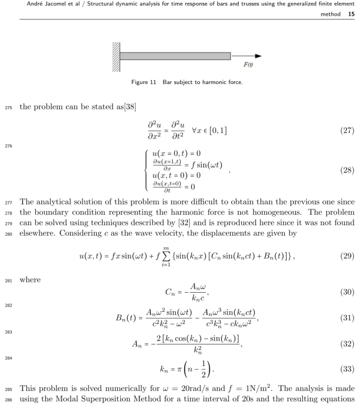
6.2 Bar subject to harmonic force
269
The second example is that of a bar fixed at one end and subject to a harmonic force at the
270
other end, as shown in Fig. 11. The properties of the material were chosen to give the wave
271
velocity equal toc=√E/ρ= 1m/s and the bar length is equal to 1m. The initial displacements
272
and velocities are zero.
273
For a force given by
274
Figure 11 Bar subject to harmonic force.
the problem can be stated as[38]
275
∂2
u ∂x2 =
∂2
u
∂t2 ∀x∈[0,1] (27) 276
⎧⎪⎪⎪⎪ ⎪⎪ ⎨⎪⎪⎪ ⎪⎪⎪⎩
u(x=0, t)=0 ∂u(x=1,t)
∂x =fsin(ωt)
u(x, t=0)=0 ∂u(x,t=0)
∂t =0
. (28)
The analytical solution of this problem is more difficult to obtain than the previous one since
277
the boundary condition representing the harmonic force is not homogeneous. The problem
278
can be solved using techniques described by [32] and is reproduced here since it was not found
279
elsewhere. Consideringc as the wave velocity, the displacements are given by
280
u(x, t)=f xsin(ωt)+f
m ∑ i=1
{sin(knx) [Cnsin(knct)+Bn(t)]}, (29)
where
281
Cn=−
Anω
knc
, (30)
282
Bn(t)=
Anω2sin(ωt)
c2k2
n−ω
2 −
Anω3sin(knct)
c3k3
n−cknω2
, (31)
283
An=−
2[kncos(kn)−sin(kn)]
k2
n
, (32)
284
kn=π(n− 1
2). (33)
This problem is solved numerically for ω = 20rad/s and f = 1N/m2
. The analysis is made
285
using the Modal Superposition Method for a time interval of 20s and the resulting equations
286
are solved using the Newmark method (with α = 0.5 and δ = 0.25) for a time step equal to
287
1.25x10⁻³
s.
288
The first comparison is made using 21 degrees of freedom. The mesh of the FEM is
289
composed of 20 linear finite elements, while the mesh of the HFEM is composed of 4 finite
290
elements of order 5. The mesh of the GFEM is composed of 4 finite elements with 4 enrichment
291
functions considering β1 = 3π/2. The analytical and the approximate solutions at x = 0.5m 292
considering 10 modes in Modal Superposition are presented in Fig. 12.
(a) (b)
(c) (d)
The errors for this example are presented in Table 3 and Fig. 13. The best result was
294
obtained with the GFEM when considering 10 modes and corresponds to an error of 0.0258.
295
The best result obtained with the HFEM was also obtained with 10 modes, but the error in
296
this case is 0.0722. The results given by the FEM are much less accurate than the results
297
obtained with the other two methods, as can be seen from Fig. 12.
298
A closer inspection of Fig. 12 reveals that the displacements obtained with the HFEM and
299
the GFEM in the time interval 0-10s are both very similar to the analytical solution. However,
300
the results given by the HFEM for the time interval 10s-20s present some deviation from the
301
analytical solution, mainly for peak displacements. The solution given by the GFEM, instead,
302
is very close to the analytical solution even in these cases.
303
Table 3 Errors obtained with 21 degrees of freedom for different numbers of modes considered in Modal Superposition.
Modes 1 2 3 4 5 6 7
FEM 1.1813 1.1823 1.2071 1.1772 1.1407 1.2813 1.1676 HFEM 1.1813 1.1820 1.2042 1.1661 1.1259 1.1876 0.1651 GFEM 1.1813 1.1820 1.2042 1.1661 1.1259 1.1876 0.1592
Modes 8 9 10 11 12 13 14
FEM 1.1948 1.2150 1.2019 1.1931 1.2000 1.2068 1.2010 HFEM 0.0778 0.0891 0.0772 0.0817 0.0801 0.0817 0.0802 GFEM 0.0530 0.0498 0.0258 0.0379 0.0320 0.0346 0.0328
Modes 15 16 17 18 19
FEM 1.1964 1.2006 1.2048 1.2005 1.1968 HFEM 0.0801 0.0801 0.0889 0.0812 0.0843 GFEM 0.0339 0.0335 0.0446 0.0351 0.0435
Figure 13 Errors obtained with 21 degrees of freedom for different numbers of modes considered in Modal Superposition.
This example is also solved using 37 degrees of freedom. The FEM mesh is composed
by 36 linear finite elements, the HFEM mesh is composed of 4 elements of order 9, and the
305
GFEM mesh is composed of two finite elements with 8 enrichment functions, by assumingβ1 306
= 3π/2 and β2 = 3π. The errors for these cases are presented in Table 4 and Fig. 14. The 307
displacements obtained using 37 degrees of freedom and 20 modes are presented in Fig. 15.
308
Table 4 Errors obtained with 37 degrees of freedom for different numbers of modes considered in Modal Superposition.
Modes 1 2 3 4 5 6 7 8 9
FEM 1.1813 1.1820 1.2045 1.1676 1.1333 1.2368 1.2341 1.2418 1.2483 HFEM 1.1813 1.1820 1.2042 1.1661 1.1259 1.1876 0.1593 0.0530 0.0494 GFEM 1.1813 1.1820 1.2042 1.1661 1.1259 1.1876 0.1593 0.0530 0.0494
Modes 10 11 12 13 14 15 16 17 18
FEM 1.2433 1.2412 1.2426 1.2447 1.2429 1.2421 1.2428 1.2439 1.2431 HFEM 0.0236 0.0284 0.0168 0.0191 0.0140 0.0169 0.0130 0.0140 0.0126 GFEM 0.0236 0.0284 0.0168 0.0191 0.0140 0.0169 0.0130 0.0139 0.0122
Modes 19 20 21 22 23 24 25 26 27
FEM 1.2425 1.2430 1.2438 1.2431 1.2426 1.2431 1.2436 1.2431 1.2427 HFEM 0.0146 0.0128 0.0134 0.0129 0.0138 0.0133 0.0146 0.0134 0.0158 GFEM 0.0141 0.0120 0.0125 0.0121 0.0131 0.0124 0.0132 0.0125 0.0148
Modes 28 29 30 31 32 33 34 35
FEM 1.2431 1.2435 1.2431 1.2427 1.2430 1.2435 1.2431 1.2428 HFEM 0.0136 0.0136 0.0136 0.0137 0.0137 0.0166 0.0137 0.0173 GFEM 0.0126 0.0126 0.0126 0.0128 0.0127 0.0164 0.0127 0.0172
From both Table 4 and Fig. 14 it can be seen that the results given by the HFEM and the
309
GFEM are very similar. The best results for both methods were obtained when considering
310
20 modes in the Modal Superposition analysis. The results given by the FEM are much less
311
accurate than the ones obtained with the other two methods.
312
The comparison between the errors obtained with the linear FEM from Table 3 and Table
313
4 indicate that the errors remained almost the same when more degrees of freedom were used.
314
Even if this result seems contradictory, since one expects the errors to be reduced when the
315
approximation is improved, the reason for this occurrence can be found by comparing the
316
displacements from Fig. 12 and Fig. 15. The overall approximation given by the FEM when
317
considering 37 degrees of freedom is better than when considering 21 degrees of freedom, except
318
at the time interval 12s-18s. From Fig. 15 it can be seen that the approximation given by the
319
FEM with 37 degrees of freedom is very poor in the time interval 12s-18s, even worse than the
320
ones obtained with 21 degrees of freedom. This increases the error in the total time interval
321
0s-20s to the same level as those observed when using 21 degrees of freedom.
Figure 14 Errors obtained with 37 degrees of freedom for different numbers of modes considered in Modal Superposition.
(a) (b)
When Modal Superposition is used, the analyst is able to improve the approximate solution
323
by removing the poorly approximated higher modes from the analysis[7], as can be observed
324
in the results of the last two examples. However, in the case that direct integration methods
325
are used one is not able to choose which modes will be considered. According to[7], direct
326
integration methods are expected to give the same results that would be obtained with Modal
327
Superposition by including all fundamental modes in the analysis. The error imbued by the
328
higher modes when using direct integration methods must then be reduced by using appropriate
329
time steps or some kind of numerical damping[7, 23].
330
In this context, the numerical damping that occurs when some time integration schemes
331
are used (note that not all time integration schemes give numerical damping) can be beneficial,
332
since the influence of the higher vibration modes (that are poorly approximated) can be damped
333
out. The Houbolt Method naturally includes some kind of numerical damping, but the analyst
334
is not able to control the magnitude of this damping[7, 23]. Some time integration schemes that
335
include numerical damping and allow the analyst to control the magnitude of this damping in
336
some way are theα-HHT method[21, 23] and the generalized-αmethod[24]. Here we use the
337
Newmark method (with α = 0.5 andδ = 0.25), that according to[7] do not cause numerical
338
damping, since we are interested in evaluating the ability of the GFEM and the HFEM to
339
approximate the higher vibration modes of the structures. The comparison of the FEM, the
340
HFEM and the GFEM together with other time integration schemes should be subject of
341
further investigation.
342
The results presented for the previous two examples indicate that the GFEM was able to
343
obtain better approximations than the HFEM and the FEM when all modes were included in
344
Modal Superposition, possibly because the higher modes have been better approximated by
345
the GFEM. This behavior plays an important role when direct integration methods are used,
346
since in this case the analyst is not able to exclude the influence of higher vibration modes
347
from the analysis.
348
6.3 Truss subject to harmonic force
349
The third example is that of the truss from Fig. 16, that is subjected to a harmonic force and
350
null initial displacements and velocities. In this case it is not possible to increase the number of
351
degrees of freedom when using the FEM with linear elements, since each bar cannot be divided
352
in two finite elements without making the structure unstable. When using the GFEM and the
353
HFEM, instead, it is possible to increase the number of degrees of freedom by increasing the
354
number of shape functions used.
355
All bars haveE = 210GPa,A= 0.005m2
,ρ= 8000kg/m3
and the truss hasL = 3m. The
356
example is solved assuming an applied force with magnitude f = 1000N and three different
357
frequencies: ω = 5000rad/s, ω = 7500rad/s and ω = 10000rad/s. No analytical solution is
358
known for this problem and it is solved only by the approximate methods. Thus no error
359
evaluation is performed and the comparison between the results is only qualitative.
360
The problem is solved using the Newmark method (withα= 0.5 andδ = 0.25) with a time
361
step equal to 1.0x10⁻⁵
s. Four different meshes are considered: a) FEM with linear elements,
F(t) = sin(ω t)
1
2
L L
L
Figure 16 Truss subject to harmonic force.
b) HFEM with 6 shape functions per bar, c) GFEM with 6 shape functions per bar, d) HFEM
363
with 10 shape functions per bar and e) GFEM with 10 shape functions per bar. All bars of the
364
structure are considered as a single finite element. In the case of the GFEM the enrichment
365
functions are obtained withβ1= 3π/2 when 6 shape functions are considered and with β1 = 366
3π/2 and β2 = 3π when 10 shape functions are considered. 367
The vertical displacements at node 1 from Fig. 16 forω = 5000rad/s are presented in Fig.
368
17. In this case it can be seen that both the HFEM and the GFEM obtained the same results
369
when using 6 and 10 shape functions per bar. The results obtained with the FEM with linear
370
elements, instead, is different from the ones obtained with the HFEM and the GFEM.
371
(a) (b)
Figure 18 Vertical displacements at node 1 forω= 7500rad/s in the time intervals a) 0s-0.01s and b) 0.01s-0.02s. The number after the name of the formulation indicates the number of shape functions used per bar.
The vertical displacements at node 1 for ω = 7500rad/s are presented in Fig. 18. The
372
HFEM and the GFEM converged to the same results when 10 shape functions per bar were
373
used and thus only the results for the HFEM with 10 shape functions are presented. Taking
374
as reference the solutions obtained with 10 shape functions per bar, a close inspection of Fig.
375
18 seems to indicate that the GFEM with 6 shape functions obtained more accurate results
376
than the HFEM with 6 shape functions. The displacements obtained with the FEM are very
377
different from the ones obtained with the other two methods.
378
The vertical displacements at node 1 for ω = 10000rad/s are presented in Fig. 19. The
379
displacements obtained with the HFEM and GFEM using 10 shape functions per bar converged
380
to the same results again. For this reason only the results given by the HFEM using 10 shape
381
functions are presented. Taking as reference the solutions obtained with 10 shape functions
382
per bar, Fig. 19 indicates that the GFEM with 6 shape functions obtained more accurate
383
results than the HFEM with 6 shape functions per bar. Besides, the difference between the
384
solutions obtained with 6 shapes functions per bar is more noticeable in this case than for ω
385
= 7500rad/s.
386
The vertical displacements at node 2 for ω = 10000rad/s are presented in Fig. 20. The
387
same conclusions drawn for the displacements at node 1 hold in this case. It seems that the
388
GFEM with 6 shape functions obtained more accurate results than the HFEM with 6 shape
389
function, taking as reference the solutions obtained with 10 shape functions per bar.
390
The comparisons made for the three different frequencies indicate that the GFEM is able
391
to obtain better results than the HFEM for higher frequencies, as observed in the previous
392
examples and by[3].
(a) (b)
Figure 19 Vertical displacements at node 1 forω= 10000rad/s for the time intervals a) 0-0.01s and b) 0.01-0.02s. The number after the name of the formulation idicates the number of shape functions used per bar.
(a) (b)
6.4 Bar subject to impact load
394
The fourth example is that of a bar subject to an impact load. The bar is initially at rest and
395
is subject to the same boundary conditions as shown in Fig. 11. The properties of the bar are
396
nowE = 210GPa, A= 0.001m2
,ρ = 8000kg/m3
and L = 1m.
397
The time dependent load is given by
398
F(t)={ f ift≤tf
0 if t>tf , (34)
where f is the force magnitude and tf is the time when the force stops. This applied force is
399
as shown in Fig. 21 and is used to model the impact load.
400
t F(t)
t
f
f
Figure 21 Impact load.
Here we assume f = 1000N and tf = 0.001s. Note that very different time responses are
401
obtained when the value of tf is changed. The problem is solved using the Newmark method
402
(with α= 0.5 and δ = 0.25) with a time step equal to 2.5x10⁻⁷
s.
403
The displacements at the middle of the bar are presented in Fig. 22. The analysis was made
404
using 11 degrees of freedom. In the case of the linear FEM, this mesh is given by dividing
405
the domain into 10 finite elements. In the case of the GFEM and the HFEM the mesh is
406
obtained by dividing the domain into 2 finite elements and assuming 6 shape functions per
407
finite element. For the GFEM β is taken equal to 3π/2. The reference solution is taken as
408
the solution given by the HFEM when using 4 finite elements with 10 shape functions. This
409
results in 37 degrees of freedom.
410
From the results presented in Fig. 22 it can be seen that the results given by the HFEM
411
and the GFEM are very close to the reference solution. The results given by the linear FEM,
412
are also able to represent the main trend of the vibration, but are not as close to the reference
413
solution. This is especially true for peak displacements and larger time intervals, as can be
414
seen in Fig. 22d. The lost of accuracy for larger time intervals appears to be reduced when
415
the HFEM and the GFEM are used.
(a)
(c)
(d)
6.5 Truss subject to impact load
417
The last example is that of the truss from Fig. 23 that is subject to an impact load. The truss
418
nodes are equally spaced and dx = dy = 2m. The material has properties E = 210GP and
419
ρ = 8000kg/m3
while all bars have a cross sectional area equal to A = 0.001m2
. There is an
420
applied force at the central node of the lower chord. This load is as defined in Eq. (34) and
421
Fig. 21, with magnitude f = 10kN andtf = 0.001s, and represents an impact load.
422
F(t) u
d
y
dx
dx
Figure 23 Truss subject to impact load.
The problem is solved using the Newmark method (with α = 0.5 and δ = 0.25) with a
423
time step equal to 1.0x10⁻⁵
s. Each bar is modeled as a single finite element. In the case of
424
the HFEM and the GFEM the analysis is made using 6 and 10 shape functions per finite
425
element. For the GFEM we assume β = 3π/2 andβ = 3π. For the linear FEM only 2 shape
426
functions are used. Note that the bars cannot be divided in two without creating an unstable
427
structure and consequently it is not possible to refine the mesh when using the linear FEM.
428
The vertical displacements at the node put in evidence in Fig. 23 are presented in Fig. 24, for
429
three different time intervals.
430
The results given by the HFEM and the GFEM with 6 and 10 shape functions cannot be
431
distinguished by visual inspection. From the time interval 0-0.01s, presented in Fig. 24a, we
432
note that the displacement wave takes some time in order to arrive at the node monitored. It
433
is also possible to see that the results given by the HFEM and the GFEM are very similar,
434
while the displacements given by the linear FEM are not coincident with the displacements
435
obtained with the other methods.
436
From Fig. 24b and Fig. 24c we note that the linear FEM is able to represent the main trend
437
of the displacements, but that accuracy is lost for larger time intervals. This lost of accuracy
438
for larger time intervals appears to be reduced when the HFEM and the GFEM are used. This
439
kind of behavior of the linear FEM can lead to difficulties for obtaining very accurate results
440
with the linear FEM, since the mesh cannot be refined just by dividing the finite elements in
441
two.
(a) (b)
(c)
7 CONCLUSIONS
443
This paper presented a GFEM formulation for the dynamic analysis of bars and trusses. The
444
time integration procedure was made using Modal Superposition and the Newmark method.
445
Numerical errors can result both from the time integration procedure and from the finite
446
element approximation. Errors from the numerical integration procedure can be reduced by
447
decreasing the time step used or by changing the number of modes considered for Modal
448
Superposition, while errors from the finite element method can be reduced by using a more
449
accurate approximation.
450
The GFEM allows one to use an enriched approximation for the displacements that is easy
451
to obtain and does not affect nodal quantities. This approximation leads to better results
452
than standard linear FEM. For the examples studied here, the GFEM also presented better
453
results than the HFEM. Besides, this GFEM formulation presented here is a hierarchical one
454
(as is the case of HFEM), since the approximation can be enriched without changing the shape
455
functions used in lower order elements. Finally, the enrichment shape functions proposed do
456
not affect the nodal degrees of freedom and thus standard procedures used for the linear FEM
457
still hold.
458
The results presented here indicate a strong potential of the GFEM for problems from
459
structural dynamics. The extension of the approach proposed in this paper to beams and two
460
dimensional problems will be subject of future works.
461
References
462
[1] Y. Abdelaziz and A. Hamouine. A survey of the extended finite element. Computers & Structures, 86:1141–1151,
463
2008.
464
[2] M.H. Aliabadi.The boundary element method: applications in solids and structures. John Wiley & Sons, Chichester,
465
2002.
466
[3] M. Arndt, R.D. Machado, and A. Scremin. An adaptive generalized finite element method applied to free vibration
467
analysis of straight bars and trusses.Journal of Sound and Vibration, 329:659672, 2010.
468
[4] Babuska, U. Banerjee, and J.E. Osborn. Generalized finite element methods: main ideas, results, and perspective.
469
Technical report, TICAM, University of Texas at Austin.
470
[5] Babuska and J.M. Melenk. The partition of unity method. International Journal for Numerical Methods in
Engi-471
neering, 40(4):727–758, 1997.
472
[6] N.S. Bardell. Free vibration analysis of a flat plate using the hierarchical finite element method. Journal of Sound
473
and Vibration, 151(2):263–289, 1991.
474
[7] K.J. Bathe. Finite element procedures. Prentice Hall, Upper Saddle River, 1996.
475
[8] E.B. Becker, G.F. Carey, and J.T. Oden. Finite elements: an introduction. Prentice-Hall, Englewood Cliffs, 1981.
476
[9] E. De Bel, P. Villon, and P. Bouillard. Forced vibrations in the medium frequency range solved by a partition of
477
unity method with local information. International Journal for Numerical Methods in Engineering, 62:1105–1126,
478
2005.
479
[10] O. Beslin and J. Nicolas. A hierarchical functions set for predicting very high order plate bending modes with any
480
boundary conditions. Journal of Sound and Vibration, 202(5):633655, 1997.
481
[11] C.A. Brebbia and D. Nardini. Dynamic analysis in solid mechanics by an alternative boundary element procedure.
482
Soil Dynamics and Earthquake Engineering, 2(4):228–233, 1983.
483
[12] F. Brezzi and M. Fortin. Mixed and hybrid finite element methods. Springer-Verlag, New York, 1991.
[13] G.F. Carey and J.T. Oden. Finite elements: a second course. Prentice-Hall, Englewood Cliffs, 1983.
485
[14] J.A.M. Carrer and W.J. Mansur. Stress and velocity in 2d transient elastodynamic analysis by the boundary element
486
method.Engineering Analysis with Boundary Elements, 23:233–245, 1999.
487
[15] A.K. Chopra.Dynamics of structures: theory and applications to earthquake engineering. Prentice Hall, Englewood
488
Cliffs, 1995.
489
[16] C. Daux, N. Moes, J. Dolbow, N. Sukumar, and T. Belytschko. Arbitrary branched and intersecting cracks with
490
extended finite element method. International Journal for Numerical Methods in Engineering, 48:1741–1760, 2000.
491
[17] C.A. Duarte and D.J. Kim. Analysis and applications of a generalized finite element method with global-local
492
enrichment functions.Computer Methods in Applied Mechanics and Engineering, 197:487–504, 2007.
493
[18] R.C. Engels. Finite element modeling of dynamic behavior of some basic structural members. Journal of Vibration
494
and Acoustics, 114:3–9, 1992.
495
[19] N. Ganesan and R.C. Engels. Hierarchical bernoulli-euller beam finite elements.Computers & Structures, 43(2):297–
496
304, 1992.
497
[20] L. Hazard and P. Bouillard. Structural dynamics of viscoelastic sandwich plates by the partition of unity finite
498
element method. Computer Methods in Applied Mechanics and Engineering, 196:4101–4116, 2007.
499
[21] H.M. Hilber, T.J.R. Hughes, and R.L. Taylor. Improved numerical dissipation for time integration algorithms in
500
structural dynamics. Earthquake Engineering and Structural Dynamics, 5:283–292, 1977.
501
[22] A. Houmat. An alternative hierarchical finite element formulation applied to plate vibrations.Journal of Sound and
502
Vibration, 206(2):201–215, 1997.
503
[23] T.J.R. Hughes. The finite element method: linear static and dynamic finite element analysis. Prentice Hall,
Engle-504
wood Cliffs, 1987.
505
[24] J.Chung and G.H. Hulbert. A time integration algorithm for structural dynamics with improved numerical dissipation:
506
the generalized- method. Journal of Applied Mechanics, 60:371–375, 1993.
507
[25] E. Kreyszig.Advanced engineering mathematics. John Wiley & Sons, Singapore, 2006.
508
[26] A.Y.T. Leung and J.K.W. Chan. Fourier p-element for the analysis of beams and plates. Journal of Sound and
509
Vibration, 212(1):179–185, 1998.
510
[27] R.J. LeVeque. Finite difference methods for ordinary and partial differential equations: steady-state and
time-511
dependent problems. SIAM, Philadelphia, 2007.
512
[28] E. Levy and M. Eisenberger. Dynamic analysis of trusses including the effect of local modes. Structural Engineering
513
and Mechanics, 7(1):81–94, 1999.
514
[29] G.R. Liu.Mesh free methods: moving beyond the finite element method. CRC Press, Boca Ratton, 2003.
515
[30] W.K. Liu, S. Jun, S. Li, J. Adee, and T. Belytschko. Reproducing kernel particle methods for structural dynamics.
516
International Journal for Numerical Methods in Engineering, 38(10):1655–1679, 1995.
517
[31] J.M. Melenk and I. Babuska. The partition of unity finite element method: Basic theory and applications.Computer
518
Methods in Applied Mechanics and Engineering, 139(1-4):289–314, 1996.
519
[32] Y. Pinchover and J. Rubinstein. An Introduction to partial differential equations. Cambridge University Press,
520
Cambridge, 2005.
521
[33] S.S. Rao. The finite element method in engineering. Elsevier, Amsterdam, 2005.
522
[34] P. Ribeiro. Hierarchical finite element analyses of geometrically non-linear vibration of beams and plane frames.
523
Journal of Sound and Vibration, 246(2):225–244, 2001.
524
[35] P. Rozycki, N. Moes, E. Bechet, and C. Dubois. X-fem explicit dynamics for constant strain elements to alleviate
525
mesh constraints on internal or external boundaries. Computer Methods in Applied Mechanics and Engineering,
526
197:349–363, 2008.
527
[36] P. Sol´ın, K. Segeth, and I. Dolezel.Higher-order finite element methods. Chapman & Hall/CRC, Boca Raton, 2004.
528
[37] Strouboulis, K. Copps, and I. Babuska. The generalized finite element method. Computer Methods in Applied
529
Mechanics and Engineering, 190:4081–4193, 2001.
[38] S. Timoshenko and J.N. Goodier. Theory of elasticity. McGraw-Hill, New York, 1951.
531
[39] A.J. Torii and R.D. Machado. Transient dynamic structural analysis of bars and trusses using the generalized finite
532
element method. InIn: E. Dvorkin, M Goldschmit and M. Storti (Eds.). Mec´anica Computacional. Buenos Aires:
533
Asociacion Argentina de Mec´anica Computacional, volume 24, pages 1861–1877, 2010.
534
[40] P. Zeng. Composite element method for vibration analysis of structure, part ii: C1 element(beam).Journal of Sound
535
and Vibration, 218(4):659–696, 1998.
536
[41] P. Zeng. Composite element method for vibration analysis of structures, part i: principle and c0 element(bar).
537
Journal of Sound and Vibration, 218(4):619–658, 1998.
538
[42] O.C. Zienkiewicz and R.L. Taylor. The finite element method, Volume 1: The Basis. Butterworth-Heinemann,
539
Oxford, 2000.