A new index for assessing the value of importance of species – VIS

Printed version ISSN 0001-3765 / Online version ISSN 1678-2690 http://dx.doi.org/10.1590/0001-3765201520140351

www.scielo.br/aabc

A new index for assessing the value of importance of species –

VIS

SYLVIO PéLLICO NETTO1

, MAURICIO K. AMARAL2

and MARCIO CORAIOLA3

1

Departamento de Engenharia Florestal, Universidade Federal do Paraná, Av. Pref. Lothário Meissner, 900, Jardim Botânico, Campus III, 80210-170 Curitiba, PR, Brasil

2

Departamento de Matemática, Universidade Tecnológica Federal do Paraná, Av. Sete de Setembro, 3165, Rebouças, 80230-901 Curitiba, PR, Brasil

3

Escola de Ciências Agrárias e Medicina Veterinária, Pontifícia Universidade Católica do Paraná, Rod. BR 376, Km14, Costeira, 83010-500 São José dos Pinhais, PR, Brasil

Manuscript received on July 3, 2014; accepted for publication on February 5, 2015

ABSTRACT

Phytosociological analysis in native forests is performed considering the horizontal and vertical structure of the studied population, whose most expressive parameters are the density, dominance, frequency, value of coverage and value of importance of species. Many phytosociological studies include a value of importance of species calculated by adding density, dominance and frequency, in their relative forms, however, this estimator is a mathematical impropriety because the result is a sum of indexes and does not express the true

meaning of species’ value. This is because the estimator is still influenced predominantly by the density

of occurrence of species and cannot capture the relevant hierarchical participation of emerging species that occur with low density in the biocoenosis. In this work, we propose a new index to characterize the value of importance of species based on the hierarchy and spatial absolute probability of the species in the biocoenosis, illustrated with data from a forest fragment of semideciduous tropical forest located in Cassia, MG, Brazil. The new index appropriately expressed the importance of species in the evaluated fragment.

Key words: light competition index, phytosociological parameters, Tropical Mixed Forest, Native Forest.

Correspondence to: Sylvio Péllico Netto E-mail: sylviopelliconetto@gmail.com

INTRODUCTION

Several ecological studies have been conducted in experimental units that form the Site ECOSILVIBRAS of the Long Term Ecological Program (PELD), today named ELFA, supported

by the Brazilian National Council of Scientific and

Technological Development (CNPq), in the Atlantic Forest, with special emphasis on forest remnants of the Araucaria Forest and its transitional areas. The

natural vegetation has been evaluated and analyzed

using taxonomic or floristic methods based on the

plant structure and physiognomy.

Floristic analyses have revealed the diversity of species that compose the arboreal stratum of the forest, and the present research work is focused on this subset of the plant population. An analysis of the horizontal structure was conducted based on the parameters of density, frequency, dominance

and cover value, reflecting the reality of the spatial

In several research studies encountered in the literature presenting evaluations of both the horizontal and vertical structures that characterize the floristic composition of forest populations, the value of importance (VIS) of species was improperly obtained considering its underlying mathematical concept. This is because the VIS was calculated as the sum of indices whose ratios do not present a common denominator.

Many authors have contributed significantly

to the development of phytosociological indices, the VIS is part of this group of indices, constituting a collection of ecological concepts that are equated biometrically and which, in most cases, are expressed by probabilistic assessments of

events of significant importance for an ecological

characterization of forests.

According to Souza et al. (1998), the tree species occurring in a forest population constitute

the essential material for a floristic analysis of a

particular area.

Phytosociological analyses are performed considering the horizontal and vertical structure of the studied population to obtain the density, dominance, frequency and value of importance, which are the most relevant parameters to describe

the structural configuration of the biocoenosis.

The density, understood as the number of individuals of each species and of all other species occurring per unit area in the studied forest population, reported in absolute quantities as absolute density (D_abs), according to Curtis and McIntosh (1950), and in relative form as relative density (D_rel), is obtained by effective counts of individuals in a continuous space and reported as a percentage (Finol 1971). If species are evaluated based on their density, called abundance by some researchers, the species are ranked as very rare, rare, occasional, abundant and very abundant, and these ranks form relevant information to characterize the composition of the forest population (Förster 1973, Longhi 1980). These factors are expressed

as D_abs =n ha. −1 for absolute density and

1 . 100

rel

D =n N− for relative density.

The dominance, understood as a measure of the total body projections of the plants (horizontal expansion), is the sum of all of the horizontal projections of the individuals belonging to one species. This concept has been applied by several researchers, including Förster (1973), Font-Quer (1975) and Longhi (1997). Martins (1991) extended this concept to the proportion of size, volume of wood or coverage of each species in relation to the space or total volume of wood occurring in the phytocoenosis. In dense forests, it becomes

difficult and complex to obtain the projection of

all of the crowns of the trees due to the peculiar vertical stratification in forests with plants of all ages. For this reason, the basal area of the entire arboreal stratum is proposed to replace the

crown’s projection area because there is significant

correlation between these two parameters (Cain et al. 1956). Finol (1971) stated that the absolute dominance (DO_abs) should be calculated as the sum of the cross-sectional areas of all trees of a given species (g ha. −1), measured at the height of 1.30 m. Similarly, the relative dominance (DO_rel), applied by Cottam and Curtis (1956), is the percentage of the basal area of each species in relation to the basal area of the entire arboreal stratum

1 1 1

. ( . )

g ha− G ha− −

The frequency is understood as the percentage of incidence of a species in the set of sample units

that were integrated into the floristic survey of a

forest population (m_i) (Förster 1973). If a species is found in all of the sample units (m), it will have a frequency of 100%. The percentage values between 0% and 100%, evaluated for each kind of population, are called absolute frequency (F_{abs i( )}) and, according to Longhi (1997), can be considered

the population sampled, informed directly as a percentage, i.e. FAi m mi 1100

−

= . The relative

frequency (F_rel) is evaluated by taking the absolute frequencies of each species F_{abs i( )} in relation to the

total of the frequencies of all of the species found in the sampling units taken in the forest population

(

∑

F_{abs i( )}), i.e. 1 ( )( ( )) 100 rel abs i abs i

F =F

∑

F − .

The value of importance (VIS), proposed by Curtis and McIntosh (1950) and used by Cottam and

Curtis (1956) and by Förster (1973), is considered a relevant estimator to order the importance of

each species in the phytocoenosis, obtained by the addition of the referred indexes, i.e.

rel rel rel

VIS

=

D

+

DO

+

F

Martins (1991) reported that the relative values of density, frequency and dominance, in isolated forms, reveal essential aspects for the characterization of the floristic composition of forests but do not indicate the structure of the

floristic vegetation as a whole. This author also

reports that the

VIS

has been of great utility to separate different types of forests and to relate them to environmental factors or even to relate the distributions of species to abiotic factors.

Braun-Blanquet (1964) described the value of coverage (

VC

) as the power of the species in the community. Also used by Förster (1973), the VC is regarded as an important index to reveal the relevance of each species in a given biocoenosis, which is obtained by the sum of the relative density and the relative dominance, i.e.

rel rel

VC

=

D

+

DO

Considering the importance that the parameter

VIS

has for ranking species in a spatial context of a tree population, a hypothetical new VIS index with appropriate mathematical rationality is viable.

Experimental data were collected to validate the new proposal.

MATERIALS AND METHODS

With the objective of proposing a new index for the value of importance (VIS) of forest species, it will be important to conceptualise each of the parameters that will be used in the calculation.

developmentofa new proposalfortHe valueof importanCe

The value of importance (

VIS

), as proposed by Curtis and McIntosh (1950) and applied by

Förster (1973), although identified as relevant to

phytosociological contextualization, constitutes a mathematical impropriety when that parameter is obtained by the sum of indices. Such a result does not express the true meaning of the index because it is still influenced predominantly by the density of occurrence of species and cannot capture the relevant hierarchical participation of emerging species that occur with low density in the biocoenosis.

The

VIS

must be obtained primarily from the dominant arboreal stratum of the biocoenosis; hence, the index of dominance is the most important parameter to be considered. The basal area of each species does not ensure dominance in the forest, and when it is incorporated to the indices of frequency and density, does not reach the aim that it is expected to express.

Dividing

g

_i by

g

produces a value termed as index of hierarchy (

IH

_i) of the species:

( )

1

1

1 1

1 1

i

n n

i i i i i

i i

IH

g n

g n

g g

−

−

− −

= =





=

_

_

=





∑

∑

(1)

Note that this index presents conditions very relevant to describe the importance of the species because it establishes, in addition to the species dominance, a clear vision of their sucessional hierarchy, i.e. the importance of their position in the arboreal stratum of the forest.

The IH can also be considered as an

appropriate indicator to express the degree of competition of species for light in the forest. The present authors propose that species can be grouped using the hierarchy index defined in (1), which considers the average hierarchical dominance of the species in the biocoenosis:

a)

IH

_i

=

0

– the species does not occur in the biocoenosis;

b)

IH

_i

<

1

– the species belongs to the lower stratum of the biocoenosis and competes severely for light;

c)

IH

_i

>

1

and

IH

_i

<

2

– the species belongs to the intermediate stratum of the biocoenosis, will express greater values of IH, and still undergoes strong competition for light;

d)

IH

_i

>

2

and

IH

_i

<

3

– the species belongs to the upper intermediate stratum of the biocoenosis, will express greater values of of IH, and undergoes moderate light competition;

e)

IH

_i

≥

3

– the species belongs to the upper stratum, is dominant, is ranked in the group of greatest importance in the biocoenosis and undergoes little competition for light.

It is important to establish the relationship of sucessional concepts with biometric ones because the hierarchy of species is the result of synecological

interactions occurring in the biocoenosis. Vieira and Higushi (1990), quoting Whitmore (1978),

confirm his statement about the behavior of native

species in the physical environment, in which he separates the occurrences of a species in clearings from those occurring in closed habitats under the canopy by the conditions of light intensity and changes in quality due to temperature increases and

saturation deficits.

There is also an increase in nutrients from the decomposition of dead individuals. Such environmental occurrences cause changes in the biological environment because existing seedlings and trees can die due to sensitivity to full light, and consequently, plants of pioneer species can appear, and other species can maximize their growth.

As suggested by Longhi (1997), the frequency of a species is considered as the probability that it occurs in the forest population. If such occurrence is reported as an absolute value, it will not result in the same value of

F

_abs if this index was obtained directly as a percentage, although the index has been called as an absolute value. To avoid misleading interpretations, we propose to identify this factor as

P

_i.

The new

VIS

was obtained by multiplying the resulting value for the

IH

_i by the value of

P

_i:

i i i

VIS

=

IH

×

P

(2)

Note that such an estimator is an index that can precisely indicate the importance of species because it allows a ranking of species considering their dominance, density and frequency in the biocoenosis. To validate this index, the results of

VIS

obtained from both of the considered methodologies were compared by means of a synthetic indicator (SI), which converts the values to the same numerical scale. These measures vary between zero (lowest score) and one (highest score), and the SI is calculated as follows:

(

)(

)

1

. . .

Sampling data were collected in a fragment of semideciduous forest located in the Reata Farm, in Cassia, MG, Brazil. Nine sampling units of 1 ha each were measured and subdivided into 100 subunits of 100 m2, totaling 9 ha in primary units and 900 subunits, in which the census was conducted.

The area is located in the municipality of Cassia, in the southern region of the state of Minas Gerais, Brazil, with approximately 200 hectares, of which approximately 90 of these of tropical semideciduous forest in climax stage, i.e. untouched, and situated between latitude 20º20’ and 20°40’ south and longitude 46°40’ and 47°00’ west.

According to Radambrasil (1978), the studied region is characterized by a morphostructural domain of remnants of ‘folded chains’, showing traces of these structures, with eventual exhibits of their emplacements. The area in question is located in the Central Highlands Region of the Alto Rio Grande, with an average altitude of approximately 680 m.

According to the Soil Survey Staff (1999),

the soils in this region are classified as dystrophic

red latosols (distrudox), mineral soils that are not hydromorphic—more specifically, typical soils with moderate average texture. The region have varied phases of semideciduous forest, a terrain that is flat or smoothly wavy and less than 90 cumulative days per year without water.

The climate of the region of Cassia, MG,

according to the Köppen classification, is type Cwa

(tropical of altitude), presenting rigorous and rainy summers, with an annual rainfall of 1200 to 1400 mm and an average annual temperatures of 26.5 ºC (maximum) and 19.5 ºC (minimum).

To test the hypothesis of goodness of fit in the

probability distributions, the Kolmogorov-Smirnov test was used. According to Scolforo (1998), this test should be preferred for the present data because other tests, such as the

G

and chi-squared,

may present biased results when the number of

observations per class is less than five.

The following hypotheses were tested for levels of 95% or 99% of probability in a bilateral test:

0

H

: The observed frequencies may adjust well to the proposed distributions.

1

H

: The observed frequencies do not adjust well to the proposed distributions.

The Kolmogorov-Smirnov test was applied to the data, and the calculated (4) and the tabulated (5) values were obtained as follows:

1

( ) ( )

cal x x x

D =SUP Fo −Fe n− (4)

1 1

2 2

95%

1.36

99%

1.63

tab tab

D

=

n

−

D

=

n

− (5)

RESULTS AND DISCUSSION

After processing the phytosociological indices, as described in the methodology for obtaining the new value of importance ((VIS) of the species, the results were calculated using data collected in 1996 from the inventory of permanent plots located in the Farm Reata (Table I). Although we have conducted annual successive measurements in these sampling units for 13 years, up to 2009, we preferred to use the results of the first measurement to support future assessments when applying the new index in dynamic studies of this forest fragment.

The absolute and synthetic values of importance (

VIS

) calculated using the methodology proposed by Curtis McIntosh were also included in Table I, for comparison with those resulting from the application of the new methodology proposed

by the first author.

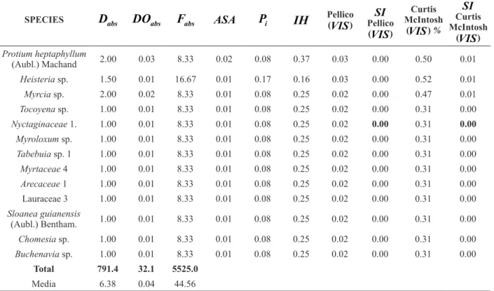
TABLE I

Results of the

VIS

proposed by Péllico Netto in a forest fragment of a semideciduous seasonal forest in the Farm Reata, Cassia, MG, Brazil.

SPECIES

D

abs

DO

abs

F

abs ASA

P

i IH

Pellico (VIS)

SI Pellico (VIS)

Curtis McIntosh

(VIS) % SI Curtis McIntosh

(VIS)

Cariniana legalis

(Mart.) Kuntze 9.25 1.44 100.00 0.16 1.00 3.84 3.84 1.00 7.47 0.49

Ficus sp. 1 2.33 0.72 50.00 0.31 0.50 7.61 3.80 0.99 3.44 0.21

Pterocarpus rohrii

Vahl 7.55 1.16 91.67 0.15 0.92 3.79 3.48 0.90 6.23 0.40

Enterolobium contortisiliquum

(Vell.) Morong.

1.00 0.53 16.67 0.53 0.17 13.07 2.18 0.57 2.08 0.12

Machaerium

aculeatum Raddi 3.00 0.50 50.00 0.17 0.50 4.11 2.06 0.53 2.84 0.17

Ficus adhatodifolia

Schott ex Spreng. 3.75 0.46 66.67 0.12 0.67 3.03 2.02 0.52 3.11 0.19

Cassia ferruginea

Schrad. ex DC. 3.38 0.36 66.67 0.11 0.67 2.63 1.75 0.45 2.75 0.17

Jacaratia spinosa

(Aubl.) A. DC. 4.80 0.39 83.33 0.08 0.83 2.00 1.67 0.43 3.33 0.21

Aspidosperma

polyneuron Mull. Arg. 1.88 0.19 66.67 0.10 0.67 2.50 1.67 0.43 2.04 0.12

Ceiba speciosa (A. St.

Hill.) Ravenna 8.78 0.79 75.00 0.09 0.75 2.22 1.66 0.43 4.93 0.32

Cariniana estrellensis

(Raddi) Kuntze 9.18 0.67 91.67 0.07 0.92 1.80 1.65 0.43 4.91 0.31

Maclura tinctoria (L.)

D. Don ex Steudel 9.91 0.72 91.67 0.07 0.92 1.79 1.64 0.42 5.15 0.33

Pseudobombax

grandiflorum (Car.) A.

Robyns

3.83 0.45 50.00 0.12 0.50 2.89 1.45 0.37 2.79 0.17

Platyciamus regnelli

Benth. 15.10 1.03 83.33 0.07 0.83 1.68 1.40 0.36 6.63 0.43

Cedrella fissilis Vell. 5.56 0.41 75.00 0.07 0.75 1.82 1.36 0.35 3.34 0.21

Lonchocarpus nitidus

(Vogel) Benth. 4.67 0.48 50.00 0.10 0.50 2.54 1.27 0.33 2.99 0.18

Alchornea triplinervia

(Spreng.) Mull. Arg. 8.88 0.62 66.67 0.07 0.67 1.72 1.15 0.30 4.26 0.27

Croton floribundus

Spreng. 55.25 1.98 100.00 0.04 1.00 0.88 0.88 0.23 14.96 1.00

Vochysia tucanorum

Mart. 1.00 0.43 8.33 0.43 0.08 10.60 0.88 0.23 1.62 0.09

Sweetia fruticosa

Spreng. 5.22 0.24 75.00 0.05 0.75 1.13 0.85 0.22 2.77 0.17

Guarea kunthiana A.

Juss. 29.67 1.26 75.00 0.04 0.75 1.05 0.79 0.20 9.03 0.60

Holocalyx balansae

Micheli 3.00 0.19 50.00 0.06 0.50 1.56 0.78 0.20 1.88 0.11

Colubrina glandulosa

TABLE I (continuation)

SPECIES

D

abs

DO

abs

F

abs ASA

P

i IH

Pellico (VIS)

SI Pellico (VIS)

Curtis McIntosh

(VIS) % SI Curtis McIntosh

(VIS)

Annona cacans Warm. 3.33 0.13 75.00 0.04 0.75 0.96 0.72 0.18 2.18 0.13

Acacia polyphylla DC 27.00 1.05 75.00 0.04 0.75 0.96 0.72 0.18 8.04 0.53

Lauraceae 5 9.00 0.31 83.33 0.03 0.83 0.85 0.71 0.18 3.61 0.23

Gallesia integrifólia

(Spreng.) Harms. 3.67 0.41 25.00 0.11 0.25 2.76 0.69 0.18 2.19 0.13

Astronium graveolens

Jacq. 34.83 0.92 100.00 0.03 1.00 0.65 0.65 0.17 9.08 0.60

Aspidosperma

pyricollum Mull. Arg. 5.50 0.86 16.67 0.16 0.17 3.86 0.64 0.16 3.68 0.23 Cabralea canjerana

(Vell.) Mart. 11.33 0.39 75.00 0.03 0.75 0.85 0.64 0.16 4.00 0.25

Chrysophyllum gonocarpum (Mart & Eichler ex Miq.) Engl.

15.36 0.41 91.67 0.03 0.92 0.66 0.60 0.15 4.88 0.31

Ormosia arborea

(Vell.) Harns. 1.50 0.11 33.33 0.07 0.33 1.81 0.60 0.15 1.14 0.06

Nectandra grandiflora

Ness. 9.00 0.29 75.00 0.03 0.75 0.79 0.60 0.15 3.40 0.21

Hymenaea courbaril L. 7.80 0.45 41.67 0.06 0.42 1.42 0.59 0.15 3.14 0.19

Aspidosperma cylindrocarpon Mull.

Arg.

4.00 0.28 33.33 0.07 0.33 1.73 0.58 0.15 1.98 0.11

Cupania vernalis

Cambess. 1.80 0.05 83.33 0.03 0.83 0.69 0.57 0.14 1.89 0.11

Cecropia

pachystachya Trecul 9.78 0.30 75.00 0.03 0.75 0.76 0.57 0.14 3.53 0.22

Ocotea odorifera

(Vell.) Rohwer 6.33 0.19 75.00 0.03 0.75 0.74 0.55 0.14 2.75 0.17

Unknown (D) 35.67 0.80 100.00 0.02 1.00 0.55 0.55 0.14 8.81 0.58

Matayba elaeagnoides

Radlk. 7.78 0.23 75.00 0.03 0.75 0.73 0.55 0.14 3.06 0.19

Cryptocarya

aschersoniana Mez 13.57 0.51 58.33 0.04 0.58 0.93 0.54 0.14 4.36 0.28

Aspidosperma

ramiflorum Mull. Arg. 6.40 0.32 41.67 0.05 0.42 1.23 0.51 0.13 2.56 0.15

Myrtaceae 1 2.29 0.08 58.33 0.04 0.58 0.86 0.50 0.13 1.59 0.09 Shefflera morototoni

(Aubl.) Maguire et al. 1.00 0.12 16.67 0.12 0.17 2.96 0.49 0.12 0.80 0.03

Siparuna apiosyce

(Mart.) DC. 7.45 0.16 91.67 0.02 0.92 0.53 0.49 0.12 3.10 0.19

Inga sp. 8.17 0.15 100.00 0.02 1.00 0.45 0.45 0.11 3.31 0.20

Trichillia claussenni

C. DC. 34.00 0.73 83.33 0.02 0.83 0.53 0.44 0.11 8.08 0.53

Clusiaceae 1 23.17 0.41 100.00 0.02 1.00 0.44 0.44 0.11 6.02 0.39

Myrsine umbellata

Mart. 1.33 0.03 75.00 0.02 0.75 0.55 0.42 0.10 1.62 0.09

Trichillia pallens C.

TABLE I (continuation)

SPECIES

D

abs

DO

abs

F

abs ASA

P

i IH

Pellico (VIS)

SI Pellico (VIS)

Curtis McIntosh

(VIS) % SI Curtis McIntosh

(VIS)

Albizia polycephalla

(Benth.) Killip 16.91 0.31 91.67 0.02 0.92 0.45 0.41 0.10 4.76 0.30

Urera bacífera (L.)

Gaudich ex Wedd. 32.33 0.69 75.00 0.02 0.75 0.53 0.39 0.10 7.59 0.50

Cordia sp. 2 3.00 0.56 8.33 0.19 0.08 4.60 0.38 0.10 2.28 0.13

Terminalia sp. 2 6.17 0.18 50.00 0.03 0.50 0.72 0.36 0.09 2.25 0.13

Trichillia sp. 14.00 0.21 91.67 0.02 0.92 0.37 0.34 0.08 4.08 0.26

Roupala montana 3.50 0.09 50.00 0.03 0.50 0.63 0.32 0.08 1.63 0.09

Copaifera langsdorffii

Desf. 8.50 0.65 16.67 0.08 0.17 1.89 0.31 0.08 3.40 0.21

Esenbeckia

grandiflora Mart. 10.42 0.13 100.00 0.01 1.00 0.31 0.31 0.08 3.53 0.22

Bauhinia forficata

Link. 8.11 0.13 75.00 0.02 0.75 0.40 0.30 0.07 2.79 0.17

Miconia discolor DC.

(Lent) 3.33 0.16 25.00 0.05 0.25 1.18 0.30 0.07 1.37 0.07

Handroanthus albus

(Cham.) Mattos 4.00 0.09 50.00 0.02 0.50 0.55 0.28 0.07 1.69 0.09

Styrax sp. 2 1.50 0.10 16.67 0.07 0.17 1.64 0.27 0.07 0.80 0.03

Trichillia pallida Sw. 8.45 0.10 91.67 0.01 0.92 0.29 0.27 0.06 3.04 0.19

Cordia sp. 3 1.00 0.13 8.33 0.13 0.08 3.21 0.27 0.06 0.68 0.03

Fabaceae 1 8.50 0.55 16.67 0.06 0.17 1.60 0.27 0.06 3.09 0.19

Lauraceae 1 1.67 0.07 25.00 0.04 0.25 1.04 0.26 0.06 0.88 0.04

Syagrus oleraceae

(Mart.) Becc 4.33 0.09 50.00 0.02 0.50 0.51 0.26 0.06 1.73 0.10 Prunus subcoriacea

(Chodat & Hassl.) Koehne

3.25 0.05 66.67 0.02 0.67 0.38 0.25 0.06 1.77 0.10

Casearia sylvestris Sw. 9.14 0.15 58.33 0.02 0.58 0.40 0.24 0.06 2.68 0.16

Zanthoxylum

rhoifolium Lam. 1.33 0.05 25.00 0.04 0.25 0.92 0.23 0.06 0.78 0.03 Zanthoxylumsp. 1.67 0.03 50.00 0.02 0.50 0.44 0.22 0.05 1.21 0.06

Aspidosperma sp. 3 2.25 0.06 33.33 0.03 0.33 0.66 0.22 0.05 1.07 0.05

Machaerium sp. 1.33 0.05 25.00 0.04 0.25 0.92 0.23 0.06 0.78 0.03

Lauraceae 4 3.00 0.06 41.67 0.02 0.42 0.49 0.21 0.05 1.32 0.07

Inga marginata Willd. 3.17 0.05 50.00 0.02 0.50 0.39 0.19 0.05 1.46 0.08

Myrtaceae 3 1.33 0.02 50.00 0.02 0.50 0.37 0.18 0.04 1.14 0.06

Allophylus sericeus

(Cambess.) Radlk. 5.60 0.10 41.67 0.02 0.42 0.44 0.18 0.04 1.77 0.10 Jacaranda micrantha

Cham. 9.25 0.20 33.33 0.02 0.33 0.53 0.18 0.04 2.40 0.14

Schinopsis brasiliensis

Engl. 2.40 0.04 41.67 0.02 0.42 0.41 0.17 0.04 1.18 0.06

Eugenia pyriformis

TABLE I (continuation)

SPECIES

D

abs

DO

abs

F

abs ASA

P

i IH

Pellico (VIS)

SI Pellico (VIS)

Curtis McIntosh

(VIS) % SI Curtis McIntosh

(VIS)

Aspidosperma sp. 2 13.25 0.26 33.33 0.02 0.33 0.48 0.16 0.04 3.09 0.19

Sorocea guilleminiana

Gaudich. 1.40 0.02 41.67 0.01 0.42 0.35 0.15 0.03 0.99 0.05

Xylopia brasiliensis

Spreng. 2.00 0.13 8.33 0.07 0.08 1.60 0.13 0.03 0.81 0.03

Aloysia virgata (Ruiz

& Pav.) Juss. 1.25 0.02 33.33 0.02 0.33 0.39 0.13 0.03 0.82 0.04

Xylopia sericea A.

St. -Hil. 4.00 0.05 41.67 0.01 0.42 0.31 0.13 0.03 1.42 0.08

Annona montana

Macfad. 4.00 0.04 50.00 0.01 0.50 0.25 0.12 0.03 1.54 0.08

Myrocarpus frondosus

Allemao 2.00 0.04 25.00 0.02 0.25 0.49 0.12 0.03 0.83 0.04

Virola sp. 3.33 0.07 25.00 0.02 0.25 0.52 0.13 0.03 1.09 0.05

Centrolobium sp. 10.67 0.20 25.00 0.02 0.25 0.46 0.12 0.02 2.42 0.14

Calophyllum

brasiliense Cambess 2.67 0.05 25.00 0.02 0.25 0.46 0.12 0.02 0.95 0.04

Senna sp.1 2.25 0.03 33.33 0.01 0.33 0.33 0.11 0.02 0.98 0.05

Ocotea sp. 1.00 0.05 8.33 0.05 0.08 1.23 0.10 0.02 0.43 0.01

Styrax sp. 1 4.33 0.07 25.00 0.02 0.25 0.40 0.10 0.02 1.22 0.06

Euterpe edulis Mart. 6.75 0.08 33.33 0.01 0.33 0.29 0.10 0.02 1.71 0.10

Rubiaceae 2 6.00 0.09 25.00 0.02 0.25 0.37 0.09 0.02 1.49 0.08

Dendropanax cuneatus

(DC.) Decne & Planch.

2.00 0.04 16.67 0.02 0.17 0.49 0.08 0.02 0.68 0.03

Rubiaceae 1 1.50 0.03 16.67 0.02 0.17 0.49 0.08 0.02 0.58 0.02

Terminalia sp. 1 1.00 0.02 16.67 0.02 0.17 0.49 0.08 0.02 0.49 0.01

Bombacopsis sp. 1.00 0.04 8.33 0.04 0.08 0.99 0.08 0.02 0.40 0.01

Casearia sp. 1.00 0.03 8.33 0.03 0.08 0.74 0.06 0.01 0.37 0.00

Nectandra

megapotamica Mez. 1.00 0.03 8.33 0.03 0.08 0.74 0.06 0.01 0.37 0.00

Citrus sp. 1.50 0.02 16.67 0.01 0.17 0.33 0.05 0.01 0.55 0.02

Aspidosperma sp. 1 4.50 0.05 16.67 0.01 0.17 0.27 0.05 0.01 1.03 0.05

Myrtaceae 5 2.00 0.02 16.67 0.01 0.17 0.25 0.04 0.01 0.62 0.02

Trema micrantha (L.)

Blume 1.00 0.01 16.67 0.01 0.17 0.25 0.04 0.01 0.46 0.01

Cordia sp. 1 1.00 0.01 16.67 0.01 0.17 0.25 0.04 0.01 0.46 0.01

Psychotria cf.

mapourioides DC. 1.00 0.01 16.67 0.01 0.17 0.25 0.04 0.01 0.46 0.01

Solanum

schwartzianum R & S. 1.00 0.01 16.67 0.01 0.17 0.25 0.04 0.01 0.46 0.01

Annona sp. 1.00 0.02 8.33 0.02 0.08 0.49 0.04 0.01 0.34 0.00

Solanum cernuum

Vell. 4.00 0.07 8.33 0.02 0.08 0.43 0.04 0.00 0.87 0.04

According to Veloso et al. (1991), the predominant vegetation in a semideciduous forest is composed of species of the genera Cariniana, Ocotea, Nectandra, Ficus, Hymenaea and Pterocarpus, which occupy the dominant stratum of the forest.

Table I facilitates a comparison of the values of

VIS

produced, using both of the methodologies contained in the present work. Note that the species with the largest

VIS

obtained by the methodology proposed by Péllico Netto was the species Cariniana legalis (Mart.) Kuntze, whereas for the methodology proposed by Curtis and McIntosh, the largest

VIS

was found for the species Croton floribundus Spreng. This difference can be explained by the clear influence of the high average absolute density (55.25 individuals. ha-1) of Croton floribundus Spreng, although this

species is not dominant in the arboreal stratum of the biocoenosis. Note that the IH of this species is equal to 0.88, which places it among the species belonging to the lower or middle stratum in the biocoenosis. In contrast, Cariniana legalis (Mart.) Kuntze, despite its lower average absolute density (9.25 individuals.ha-1), presents a value of IH

equal to 3.84, i.e. Cariniana legalis ranks among the species belonging to the upper stratum, where some species are dominant and participate in the group of greatest importance of the biocoenosis.

Anyone who knows the climax condition of the sampled fragment, which contains trees more than 2000 years old, would agrees that the

VIS

proposed by Péllico Netto appropriately ranks the species that dominate the upper strata of the biocoenosis. This is because both Ficus sp. and Pterocarpus rohrii Vahl, the second and third species with TABLE I (continuation)

SPECIES

D

abs

DO

abs

F

abs ASA

P

i IH

Pellico (VIS)

SI Pellico (VIS)

Curtis McIntosh

(VIS) % SI Curtis McIntosh

(VIS)

Protium heptaphyllum

(Aubl.) Machand 2.00 0.03 8.33 0.02 0.08 0.37 0.03 0.00 0.50 0.01

Heisteria sp. 1.50 0.01 16.67 0.01 0.17 0.16 0.03 0.00 0.52 0.01

Myrcia sp. 2.00 0.02 8.33 0.01 0.08 0.25 0.02 0.00 0.47 0.01

Tocoyena sp. 1.00 0.01 8.33 0.01 0.08 0.25 0.02 0.00 0.31 0.00

Nyctaginaceae 1. 1.00 0.01 8.33 0.01 0.08 0.25 0.02 0.00 0.31 0.00 Myroloxum sp. 1.00 0.01 8.33 0.01 0.08 0.25 0.02 0.00 0.31 0.00

Tabebuia sp. 1 1.00 0.01 8.33 0.01 0.08 0.25 0.02 0.00 0.31 0.00

Myrtaceae 4 1.00 0.01 8.33 0.01 0.08 0.25 0.02 0.00 0.31 0.00

Arecaceae 1 1.00 0.01 8.33 0.01 0.08 0.25 0.02 0.00 0.31 0.00

Lauraceae 3 1.00 0.01 8.33 0.01 0.08 0.25 0.02 0.00 0.31 0.00

Sloanea guianensis

(Aubl.) Bentham. 1.00 0.01 8.33 0.01 0.08 0.25 0.02 0.00 0.31 0.00

Chomesia sp. 1.00 0.01 8.33 0.01 0.08 0.25 0.02 0.00 0.31 0.00

Buchenavia sp. 1.00 0.01 8.33 0.01 0.08 0.25 0.02 0.00 0.31 0.00

Total 791.4 32.1 5525.0

Media 6.38 0.04 44.56

abs

the highest

VIS

values, are distinguished by the presence of lush representatives in the biocoenosis, with

dbh

1

≥

.00

m

, giving these species IH values of 7.61 and 3.79, respectively. Such hierarchical positions are superior to that obtained by Cariniana legalis (Mart.) Kuntze; however, Ficus sp. and Pterocarpus rohrii cannot surpass Cariniana legalis because they occur with lower densities in the biocoenosis.

Additionally, the two species with the second and third positions of

VIS

in the methodology proposed by Curtis and McIntosh: Astronium graveolens Jacq. and Guarea kunthiana Juss., which stand out for their high densities but have

IH values of 0.65 and 1.05, respectively, are positioned in the lower or intermediate stratum of the biocoenosis.

The species Enterolobium contorstisiliquum Morong. and Vochysia tucanorum Mart., despite their low average occurrence in the biocoenosis, are distinguished by the presence of many individuals of large size, i.e. that reach

DO

_abs of 0.53 m2.ha-1 and 0.43 m2.ha-1, respectively. These species presented average

dbh

of 0.82 m and 0.70 m, respectively, and for this reason, they reached to the highest hierarchical level of the species, with

IH values of 13.07 and 10.60, respectively. The new index proposed to assess the value of importance – (

VIS

) of species is the result of an initial assessment of the Index of Hierarchy (IH), which considers the average individual dominance of each species and, subsequently, is weighted by the probability of the spatial occupation (

P

_i) of each species in the biocoenosis.

The results obtained by the application of the new index value of importance (

VIS

) show a coherent reality of the species participation in the biocoenosis because the structure of the assessed forest fragment has already reached a climax stage.

To facilitate a comparison of the importance of the species, a new

VIS

was calculated on a scale from zero to one, denominated as

VIS

synthetic,

which started with the species Cariniana legalis (Mart.) Kuntze, with the value 1.00, and ended with the species Buchenavia sp., with the value 0.00.

Analyzing the frequency distribution of the

VIS

values in the forest fragment, it was possible to distinguish four groups of species in order of importance:

• Group I - With VIS between 0.9 - 1.0: Cariniana legalis, Ficus sp. 1 and Pterocarpus rohrii;

• Group II - With VIS between 0.4 - 0.6: Enterolobium contorstiliquum, Machaerium aculeatum, Ficus sp. 2, Cassia ferruginea, Jacaratia spinosa, Aspidosperma polyneuron, Chorisia speciosa, Cariniana estrellensis and Macuria tinctoria;

• Group III - With VIS between 0.2 - 0.4: Pseudobombax grandiflorum, Platyciamus regnelli, Cedrella fissilis, Lonchocarpus sp., Anchornea triplinervia, Croton floribundus, Volchysia tucanorum, Caesalpinaceae 1, Guarea kunthiana, Holocalix balansae and Columbrina grandulosa;

• Group IV - With VIS between 0.0 - 0.2: the remaining 102 species. The non-occurrence of species with VIS in the range between 0.6 and 0.9 means that the successional process is in progress because the related species in Group II have the possibility of expanding their dominance. The species in Group II present, except Enterolobium contorstisiliquum Morong., a probability to occupy space in the biocoenosis (Pi ≥ 0.5). Observing the groups, 75.5% of the species are allocated in Group IV, indicating a remarkable potential for species growth, which will ensure a dynamic successional process in the next few decades, in spite of this forest fragment has already reached its climax stage.

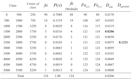
Log-TABLE II

Adjustment and evaluation of Weibull-3P distribution of the average cross-sectional area of all of the studied species (cm2

).

Class Center of

class fo P x( ) fe

(Weibull) ( )x

Fo Fe_{( )x}

D

_calc Dtab;0.05

0 500 250 90 0.7088 88 90 88 0.0170

0.1221

500 1000 750 18 0.1519 19 108 107 0.0103

1000 1500 1250 8 0.0629 8 116 115 0.0119

1500 2000 1750 5 0.0316 4 121 118 0.0206

2000 2500 2250 0 0.0176 2 121 121 0.0030

2500 3000 2750 0 0.0105 1 121 122 0.0075

3000 3500 3250 1 0.0065 1 122 123 0.0059

3500 4000 3750 0 0.0042 1 122 123 0.0101

4000 4500 4250 1 0.0028 0 123 124 0.0049

4500 5000 4750 0 0.0019 0 123 124 0.0067

5000 5500 5250 1 0.0013 0 124 124 0.0000

Total 124 1.00 124 0.0206

TABLE III

Result of the coefficients and the accuracy of the adjustment of the Weibull-3P

for the average cross-sectional area of all the studied species (cm2).

Regression Statistics Parameters of the Weibull distribution R2

0.9986 a 107.1

Standard Error 1.0305 b 300.0

Standard Error (%) 0.2089 c 0.6

normal and Weibull-3P were adjusted to the data of the forest fragment. The Weibull-3P distribution

was chosen because of its goodness of fit, as is

presented in Table II.

The Weibull-3P function, according to the model presented in (6), was fitted using the maximum

likelihood method, and the coefficient values are

presented in Table III and illustrated in Figure 1.

(

)

( )

(

)

₁ ( ) 1

1 1

c

c ATM a b

f ATM

cb

ATM

a b

exp

−

− − − 

−

_

−

_

 

=

_

−

_

(6)

Where

0

≤ <

a

ATM

_min

;

ATM

_min

>

0;

b e c

>

0

(

)

(

)

1

1 1

0

1 1 1 1

c

k k k k

c

i i

i i i i

c

f ln ATM

a

fo

and b

fo ATM

a

fo

− −

= = = =











_

_











=

_

−

_

_

_

_

=



_

−

_

_

_

_

_











The probabilities of species dominance analyzed as a function of the random variable (average of cross-sectional area (ACA) for all of the species) show that 71% of the species do not exceed 0.05 m2.ha-1, i.e. the average maximum diameter corresponding to the average cross-sectional area is equal to 25 cm; 15% of the studied species can reach 0.10 m2_.ha-1_{, i.e. the average maximum} diameter corresponding to the average cross-sectional area is equal to 35.68 cm; and only 0.13% of the species dominate the biocoenosis because they can reach up to 0.55 m2_.ha-1_{, i.e. the diameter} corresponding to the average cross-sectional area is equal to 83.68 cm. Although a well-known tree of Cariniana legalis (Mart.) Kuntze was not included in the present sampling, its dbh was measured and is equal to 243 cm.

The residuals were defined assuming normality of the errors Zi ~N(0,1), in which

(

)( )

1

ˆ

i i e

Z = e −e

σ

−, whose graph was constructed from this standardization of the estimated transformed values of the average of cross-sectional areas by species, adding one to all observed and estimated frequencies to eliminate

zero occurrences. The range of variation of residues along the ordinate axis is within the interval

(

µ

−3 ;

σ µ

+3

σ

)

, indicating that there is a linear relationship between the observed values and those estimated from the Weibull-3P distribution, which

confirms the absence of discrepancies among the

residuals (Fig. 2).

CONCLUSIONS

Considering the new methodology for the hierarchy of species, the authors propose that the studied fragment of the semideciduous forest should be ecologically characterized by the species with

2

IH

≥

because these species effectively represent the upper stratum, are dominant and form the group of greatest importance in the biocoenosis: Enterolobium contortisiliquum (Vell.) Morong. (13.07), Vochysia tucanorum Mart. (10.60), Ficus sp. 1 (7.61), Cordia sp. 2 (4.60), Machaerium aculeatum Raddi (4.11), Aspidosperma pyricollum Mull. Arg. (3.86), Cariniana legalis (Mart.) Kuntze (3.84), Pterocarpus rohrii Vahl (3.79), Cordia sp. 3 (3.21), Ficus sp. 2 (3.03), Shefflera sp. (2.96), Pseudobombax grandiflorum (Car.) A. Robyns

0 10 20 30 40 50 60 70 80 90 100

250 750 1250 1750 2250 2750 3250 3750 4250 4750 5250

F

re

q

u

en

cy

Average cross-sectional area per species (cm2₎

Observed frequency Weibull 3P distribution

(2.89), Gallesia integrifolia (Spreng.) Harms. (2.76), Cassia ferruginea Schrad. ex DC. (2.63), Lonchocarpus nitidus (Vogel) Benth. (2.54), Aspidosperma polyneuron Mull. Arg. (2.50), Ceiba speciosa (A. St. Hill.) Ravenna (2.22) and Jacaratia spinosa (Aubl.) A. DC. (2.00).

RESUMO

Análise fitossociológica em florestas nativas é

realizada considerando a estrutura horizontal e vertical da população estudada, cujos parâmetros mais expressivos são a densidade, dominância, frequência, valor de cobertura e valor de importância das espécies.

Muitos estudos fitossociológicos incluem um valor

de importância das espécies calculado adicionando-se densidade, dominância e frequência, em suas formas relativas, no entanto, este estimador é uma impropriedade matemática porque o resultado é uma

soma de índices e não expressa o verdadeiro significado

do valor das espécies. Isto ocorre porque o estimador

continua sendo influenciado principalmente pela

densidade de ocorrência de espécies e não consegue captar a participação hierárquica relevante de espécies emergentes que ocorrem com menor densidade na biocenose. Neste trabalho, propomos um novo índice para caracterizar o valor de importância das espécies com base na hierarquia e probabilidade absoluta espacial das espécies na biocenose, ilustrado com dados de um fragmento de Floresta Estacional Semidecidual localizada em Cassia, MG, Brasil. O novo índice

adequadamente expressa a importância de espécies no fragmento avaliado.

Palavras-chave: Índice de competição por luz, parâmetros

fitossociológicos, Floresta Estacional Semidecidual,

Floresta Nativa.

REFERENCES

Braun-Blanquet J. 1964. Pflanzensoziologie; Grundzüge der Vegetationskunde. Wien, New York, Springer-Verlag, 865 p.

Cain sa, Castro Gm, pires Jm and silva nt. 1956. Application of some phytosociological techniques to Brazilian rain forest. Am J Bot 43(10): 911-941.

Cottam G and Curtis Jt. 1956. The use of distance measures in phytosociological sampling. Ecology 37(3): 451-460.

Curtis Jt and mCintosH rp. 1950. The interrelations of certain analytic and synthetic phytosociological characters. Ecology Tempe 31(3): 434-450.

finol H. 1971. New parameters to be considered in the structural analysis of tropical rainforests. (Nuevos parámetros a considerarse en el análisis estructural de las selvas virgenes tropicales). Rev For Venez 14(21): 29-42.

font-quer p. 1975. Dictionary of Botany. Editorial Labor, S.A., Barcelona-Madrid. Diccionário de Botánica, 1244 p.

försterm. 1973. Strukturanalyse eines tropischen Regenwalds in Kolumbien. Allg Forst J Stg Wien 144(1): 1-8.

lonGHi sJ. 1980. A estrutura de uma floresta natural da Araucaria angustifolia (Berth.) Kuntze, no sul do Brasil. Curitiba: UFPR, 1980. Dissertação (Mestrado em Engenharia Florestal) – Universidade Federal do Paraná, 198 p. (Unpublished).

lonGHi sJ. 1997. Agrupamento e análise fitossociológica de comunidades florestais na sub-bacia hidrográfica do Rio

-2.5 -2 -1.5 -1 -0.5 0 0.5 1 1.5 2 2.5

250 750 1250 1750 2250 2750 3250 3750 4250 4750 5250

S

ta

n

d

ar

d

r

es

id

u

es

Linear of average cross-sectional area per species (expected)

Passo Fundo – RS. Curitiba: UFPR, 1997. Tese (Tese de Doutorado) – Universidade Federal do Paraná, 198 p.

martins fr. 1991. Estrutura de uma floresta mesófila. 2a

ed., São Paulo: Editora da UNICAMP, 246 p.

radamBrasil. 1978. Levantamento de Recursos Naturais 23: 742.

sColforo Jrs. 1998. Modelagem do crescimento e da produção de florestas plantadas e nativas. UFLA/FAEPE, Lavras, p. 451.

soil survey staff. 1999. Soil Taxonomy: a basic system of soil classification for making and interpreting soil surveys. USDA-NRCS Agricultural Handbook 436. 2nd

ed., U.S. Government Printing Office, Washington, D.C.

souza al, meira netoJAAand sCHettino s. 1998. Avaliação florística, fitossociológica e paramétrica de

fragmento de floresta atlântica secundária, município de Pedro Canário, Espírito Santo. Viçosa: SIF, 117 p. (Doc. SIF, 18)

veloso Hp, ranGel-filHoALRand limaTCA. 1991. Classificação da vegetação brasileira, adaptada a um sistema universal. Rio de Janeiro, IBGE. (Departamento de Recursos Naturais e Estudos Ambientais), 123 p.

vieira G and HiGusHi n. 1990. Efeito do tamanho de clareira na regeneração natural em floresta mecanicamente explorada na Amazônia brasileira. In: Congresso Florestal Brasileiro, 6º. Campos do Jordão. Anais. São Paulo: s.n., 3: 666-672.