André Pires Alves
Licenciado em Engenharia Informática
Best Photo Selection
Dissertação para obtenção do Grau de Mestre em
Engenharia Informática
Orientador: Fernando P. Birra, Prof. Auxiliar,
Faculdade de Ciências e Tecnologia da Universidade Nova de Lisboa
Co-orientador: João M. Lourenço, Prof. Auxiliar,
Faculdade de Ciências e Tecnologia da Universidade Nova de Lisboa
Júri
Presidente: Prof. Artur Miguel Dias, FCT UNL Arguente: Prof. Rui Nóbrega, FEUP
Best Photo Selection
Copyright © André Pires Alves, Faculdade de Ciências e Tecnologia, Universidade NOVA de Lisboa.
A Faculdade de Ciências e Tecnologia e a Universidade NOVA de Lisboa têm o direito, perpétuo e sem limites geográficos, de arquivar e publicar esta dissertação através de exemplares impressos reproduzidos em papel ou de forma digital, ou por qualquer outro meio conhecido ou que venha a ser inventado, e de a divulgar através de repositórios científicos e de admitir a sua cópia e distribuição com objetivos educacionais ou de inves-tigação, não comerciais, desde que seja dado crédito ao autor e editor.
A c k n o w l e d g e m e n t s
First and foremost, I would like to express my gratitude to my advisers, Prof. Fernando Birra and Prof. João Lourenço, for the opportunity of letting me work and explore this project and also for their patience, support and guidance through its course.
I would also like to express my appreciation to Departamento de Informática da Faculdade de Ciências e Tecnologia da Universidade Nova de Lisboa (DI - FCT/UNL) for being like a second home during my academic journey and also for allowing me to become a better person, not only professionally but also as a human being.
To my family, particularly my parents and grandfather, for always being there for me. Their endless encouragement, support and love gave me the strength to go through this hard path.
A b s t r a c t
The rising of digital photography underlies a clear change on the paradigm of the pho-tography management process by amateur photographers. Nowadays, taking one more photo comes for free, thus it is usual for amateurs to take several photos of the same subject hoping that one of them will match the quality standards of the photographer, namely in terms of illumination, focus and framing. Assuming that the framing issue is easily solved by cropping the photo, there is still the need to select which of the well framed photos, technically similar in terms of illumination and focus, are going to be kept (and in opposition which photos are going to be discarded). The process of visual observation, on a computer screen, in order to select the best photo is inaccurate and thus becomes a generator of insecurity feelings that may lead to no discarding of photos at all. In this work, we propose to address the issue of how to help the amateur photographer to select the best photo from a set of similar photos by analysing them in technical terms. The result is a novel workflow supported by a software package, guided by user input, which will allow the sorting of the similar photos accordingly to their technical charac-teristics (illumination and focus) and the user requirements. As a result, we expect that the process of choosing the best photo, and discarding of the remaining, becomes reliable and more comfortable.
Keywords: Signal Processing, Image Processing, Decisions Support Systems, Digital
R e s u m o
O aparecimento da fotografia digital está na base de uma clara mudança de paradigma no processo de gestão da fotografia por amadores. Porque tirar mais uma fotografia agora não representa qualquer custo adicional, é habitual tirarem-se múltiplas fotografias ao mesmo sujeito, na expectativa de que uma delas corresponda aos padrões de qualidade desejados, em termos de iluminação, foco e enquadramento. Assumindo que a questão do enquadramento se resolve facilmente recorrendo ao recorte (crop) da fotografia, tem-se ainda assim que selecionar qual das várias fotografias bem enquadradas, tecnicamente parecidas em termos de iluminação e foco, vamos guardar (e por oposição quais vamos descartar). A escolha da melhor fotografia com base na observação visual em ecrã de computador é um processo muito pouco preciso e, portanto, gerador de sensações de insegurança que resultam, muitas vezes, na opção de não descartar nenhuma das várias fotografias semelhantes. Neste trabalho propomo-nos endereçar a questão de como ajudar um fotógrafo amador a selecionar a melhor fotografia, de um conjunto, analisando-as em termos técnicos. Propomos assim uma solução inovadora para este problema específico, baseada num processo (workflow) suportado por um pacote desoftware, que com alguma ajuda do utilizador permite ordenar um conjunto de fotografias semelhantes de acordo com as suas características técnicas (iluminação e foco), permitindo assim escolher aquela que melhor corresponde às expectativas e dando segurança e conforto na eliminação das restantes.
C o n t e n t s
List of Figures xvii
List of Tables xix
Listings xxi
1 Introduction 1
1.1 Context & Motivation . . . 1
1.2 Problem Description & Objectives . . . 1
1.2.1 Improper Focus . . . 2
1.2.2 Camera & Motion Blur . . . 2
1.2.3 Noise . . . 3
1.2.4 Uneven Exposure . . . 3
1.2.5 Unrealistic Colour Cast . . . 4
1.2.6 Best Photo Selection . . . 4
1.3 Research Question & Approach . . . 5
1.4 Contributions . . . 6
1.5 Publications . . . 6
1.6 Document Organization . . . 6
2 Background & Related Work 7 2.1 Fundamental Concepts of Photography . . . 7
2.1.1 Light . . . 8
2.1.2 Exposure . . . 8
2.1.3 Focus Points . . . 8
2.1.4 Aperture . . . 9
2.1.5 Depth of Field . . . 9
2.1.6 Shutter Speed . . . 9
2.1.7 ISO . . . 11
2.1.8 Level of Exposure . . . 12
2.1.9 White Balance . . . 12
2.2 Image Correlation Algorithms . . . 13
CO N T E N T S
2.2.2 Keypoint Matcher . . . 14
2.3 Focus Detection Algorithms . . . 15
2.3.1 Fourier Transform . . . 15
2.3.2 Wavelet Transform . . . 16
2.3.3 Focus Quality Classification . . . 16
2.4 Motion Blur Detection Algorithms . . . 18
2.4.1 Image Gradient . . . 18
2.4.2 Blur Detection & Classification . . . 19
2.5 Noise Detection Algorithms . . . 22
2.5.1 Filtering-based Detection . . . 22
2.5.2 Block-based Detection . . . 22
2.6 Colour Analysis . . . 23
2.6.1 Colour Space . . . 23
2.6.2 Colour Temperature . . . 24
2.6.3 Histogram Processing . . . 24
2.7 Photo Quality Estimation . . . 24
2.7.1 Automatic Photo Selection for Media and Entertainment Applica-tions . . . 24
2.7.2 Tiling Slideshow . . . 25
2.8 Image Processing Applications . . . 26
2.8.1 Adobe Bridge . . . 26
2.8.2 Adobe Lightroom . . . 26
2.8.3 Capture One . . . 27
2.8.4 DxO Optics Pro . . . 27
2.8.5 Google+ . . . 27
2.8.6 Photo Mechanic . . . 28
2.8.7 Discussion . . . 28
2.9 OpenCV . . . 28
3 System Description & Features 31 3.1 System Description . . . 31
3.1.1 Concept . . . 31
3.1.2 Workflow . . . 32
3.2 Features . . . 33
3.2.1 Image Correlation . . . 34
3.2.2 Focus Detection . . . 43
3.2.3 Motion Blur Detection . . . 48
3.2.4 Noise Estimation . . . 52
3.2.5 Colour Analysis . . . 56
4 Conclusions & Future Work 63
4.1 Conclusions . . . 63
4.2 Future Work . . . 64
Bibliography 65 A Image Correlation Results 69 A.1 Histogram Equalization . . . 69
A.2 SIFT & SURF Comparison . . . 70
A.3 FLANN . . . 71
B Focus Detection Results 75 C Noise Estimation Results 79 C.1 Filtering-based Method . . . 80
C.2 Entropy-based Method . . . 81
D Exposure Level Results 85 E Code Snippets 87 E.1 Image Correlation . . . 87
E.1.1 Keypoint Detection . . . 87
E.1.2 Keypoint Matching . . . 87
E.2 Focus Detection . . . 88
E.3 Motion Blur . . . 90
E.4 Noise Estimation . . . 90
E.4.1 Filtering-based Method . . . 90
E.4.2 Entropy-based Method . . . 90
L i s t o f F i g u r e s
2.1 Point of focus on the flower petals (a) and point of focus on the flower stalk (b). 9
2.2 Local focus (left side) and global focus (right side). . . 10
2.3 Slow shutter speed combined with panning the camera(a); Slow shutter speed but no panning of the camera(b). . . 10
2.4 Blurry image due to camera shake(a); expected result (b). . . 11
2.5 Difference between an image with ISO value of 100 (a) and 3200 (b). . . . 11
2.6 Difference between underexposed image (a), the ideal exposure (b) and an overexposed image (c). . . 12
2.7 Top portion iscold. Bottom section iswarm. Middle section shows a correct white balance setting for the image. . . 13
2.8 Different edge types. . . . 20
2.9 Filtering-based noise estimation schematic. . . 23
3.1 Workflow schematic. . . 32
3.2 Proceeding overview for image correlation. . . 34
3.3 Underexposed image before histogram equalization (a) and respective his-togram of colour intensities (from 0 to 255) (b). . . 35
3.4 Underexposed image after histogram equalization (a) and respective histogram of colour intensities (from 0 to 255) (b). . . 35
3.5 Histogram equalization impact on keypoint detection using SIFT. . . 36
3.6 Comparison of SIFT and SURF in keypoint detection. . . 36
3.7 Comparison of SIFT and SURF in processing times. . . 37
3.8 Result of SURF algorithm. . . 38
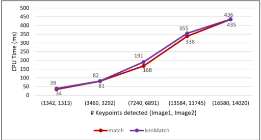
3.9 FLANN:matchandknnMatchcomparison on the matching process. . . 39
3.10 FLANN:matchandknnMatchcomparison on processing time. . . 39
3.11 Methodmatchusing 2∗min_distas a global threshold. . . 40
3.12 MethodknnMatchusing 1/1.5 as a local threshold. . . 40
3.13 FLANN: Three false matches marked in red colour. . . 41
3.14 Image correlation after the homography estimation (1). . . 41
3.15 Image correlation after the homography estimation (2). . . 41
3.16 HSV cone. . . 42
L i s t o f F i g u r e s
3.18 Approach overview in focus detection. . . 44
3.19 Differently focused images . . . . 44
3.20 Sobel output (inverted colours). . . 45
3.21 Proceeding result for different slider values. . . . 45
3.22 ROI selection. . . 46
3.23 ROIs obtained. . . 46
3.24 Segmentation result: pixels inside the polygons are represented in white colour. 47 3.25 Impact of the image technical characteristics on the gradient. . . 48
3.26 Sobel execution time (milliseconds) on different image resolutions. . . . 49
3.27 Motion blur example . . . 49
3.28 Edges detected in Figure 3.27 (inverted colours). . . 50
3.29 Image divided intoN xNregions. . . 50
3.30 Result of the Hough Transform (inverted colours). . . 51
3.31 Directional histograms of Figures 3.30(a) and 3.30(b). . . 52
3.32 Three images taken with different ISO values and respective hue colour chan-nels. . . 54
3.33 Noise estimation results. . . 54
3.34 Image containing 16.7 million colours. . . 55
3.35 Synthetic noise added to Figure 3.34. . . 55
3.36 Processing times (ms) for entropy-based and filtering-based methods. . . 56
3.37 HSV cone. . . 57
3.38 Brightness values for different level of exposure. . . . 58
3.39 Similar images containing different white balance settings. . . . 58
3.40 Respective points automatically detected in different images. . . . 59
3.41 Coldandwarmcolours. . . 59
3.42 Processing times (ms) for exposure level estimation. . . 60
A.1 Impact ofcontrastThreshold(SIFT) andhessianThreshold(SURF) on processing time (ms) and keypoint detection. . . 71
B.1 Differently exposed images used for gradient testing. . . . 76
L i s t o f Ta b l e s
2.1 Light sources temperature. . . 24
3.1 Entropy-based method results for Figure 3.34. . . 56
3.2 Saturation and hue values for different white balance settings. . . . 59
A.1 Results for a balanced exposure. . . 69
A.2 Results before histogram equalization (underexposed image). . . 69
A.3 Results after histogram equalization (underexposed image). . . 70
A.4 Comparison of SIFT and SURF in keypoint detection. . . 70
A.5 Comparison of SIFT and SURF in processing times. . . 71
A.6 SIFT: Impact ofcontrastThresholdon processing times (ms) and keypoint de-tection. . . 72
A.7 SURF: Impact ofhessianThresholdon processing times (ms) and keypoint de-tection. . . 72
A.8 FLANN results using methodmatch. . . 72
A.9 FLANN results using methodknnmatch. . . 73
B.1 Impact of the image technical characteristics on the gradient. . . 75
B.2 Sobel execution time (milliseconds) on different image resolutions (megapixels). 76 C.1 Comparison of entropy-based and filtering-based methods in processing times. 79 C.2 Noise estimation results for Set 1 (filtering-based method). . . 80
C.3 Noise estimation results for Set 2 (filtering-based method). . . 80
C.4 Noise estimation results for Set 3 (filtering-based method). . . 81
C.5 Noise estimation results for Set 4 (filtering-based method). . . 81
C.6 Noise estimation results for Set 1 (entropy-based method). . . 82
C.7 Noise estimation results for Set 2 (entropy-based method). . . 82
C.8 Noise estimation results for Set 3 (entropy-based method). . . 83
C.9 Noise estimation results for Set 4 (entropy-based method). . . 83
L i s t i n g s
E.1 Code for keypoint detection using SURF algorithm . . . 87
E.2 Code for keypoint description using SURF algorithm . . . 88
E.3 Code for keypoint matching using FLANN library . . . 88
E.4 Code for outlier removal using RANSAC method . . . 89
E.5 Code for focus analysis . . . 89
E.6 Code for applying a mask over the image focused regions . . . 90
E.7 Code for motion blur detection . . . 91
E.8 Code for noise estimation using filtering-based method . . . 91
E.9 Code for noise estimation using entropy-based method . . . 92
C
h
a
p
t
e
1
I n t r o d u c t i o n
1.1 Context & Motivation
Photography can be defined as the art and science of recording images by means of capturing light on a light-sensitive medium [Per08]. The earliest known permanent photography, recognized as theView from the Window at Le Gras(c. 1826), was taken by Nicéphore Niépce (1765-1833) having an approximate 8 hour exposure [Ros97].
After the Niépce’s discovery, photography has evolved greatly culminating into digital photography, created by digital cameras, which awards photographers with novel ways to explore and master new light capturing techniques.
The ever growing research in fields such as computer vision and image processing promote the union between the world of computer science and the world of photogra-phy, leading to numerous image editing techniques and software products that aim at providing assistance to the photographer’s task of manipulating their images.
It was estimated that in the year of 2012 alone, over 15 million digital single lens reflex (DSLR) cameras were sold [Gri]. Also, by 2010 Adobe predicted that there were over 10 million Photoshop users worldwide [Ado]. Such facts give the ideal motivation for the creation or reinvention of workflows that explore the world of photography and thus simplify the photographer’s life.
1.2 Problem Description & Objectives
Light is a vital component within the art of photography since it makes the image regis-tration by the camera sensor possible. Registering the light of a scene with the sensor of a DSLR camera may lead to very different results, varying on factors such as sharp focused
C H A P T E R 1 . I N T R O D U C T I O N
film photography, may be stored in reusable memory cards with advantages, for instance, in cost terms. Consequently, to increase the probability of achieving the desired result it is a common practice among amateur photographers to take several shots of the same subject, in automatic mode, hopping that one of them will match their quality require-ments. Good lighting, clear center of interest, no shaking, absence of noise or a good composition can be among the desired requirements. Combining such requirements may be hard to achieve in a single photo as a series of unsought effects may occur due to a
wrong use, or misinterpretation, of the camera settings.
1.2.1 Improper Focus
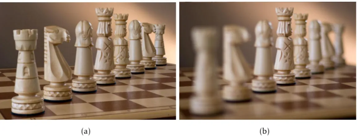
While taking photos, the photographer may choose to capture an image where all the details are acceptably focused, for instance a landscape photo, or may opt to focus a specific subject leaving it sharply focused with the remainder of the image blurred.
However, the process of focusing a specific subject may be not always successful. An improper focus may occur due to photographer’s mistakes such as bad focus points adjustment, leaving the focus points away from the subject, or a wrong definition of the range of distance (depth of field) that is in sharp focus. On the other hand, the photographer may be trying to capture an image where the subject is slightly moving, like a flower in a windy day or a restless child making it difficult to set the points of focus
on the desired area.
The focused area is the one that attracts the most attention from the viewer, a photo in which the center of interest is not sharply focused becomes undesirable. Therefore, the focusing process may be considered one of the most relevant at the image capturing moment.
1.2.2 Camera & Motion Blur
When photographers capture images focusing on a specific subject, the remaining details appear blurred thereby emphasizing the main subject. Nevertheless, blur can also occur in other situations that bring a negative impact to the photo.
The first case, and the most critical one, happens when the camera moves during the image capturing time frame. The phenomenon of camera blur is due to simple factors such as trembling of hands or breathing of the photographer or even the simple pressing of the camera button, being specially sensitive for longer exposure times. As a result, the photo contains an image that shows general blur, with no clear center of interest, being certainly short from the expected result.
require some expertise and technical skills from the photographer, and are very hard to achieve by the common amateur photographer. A wrong definition of the exposure time can result in a photo where the subject of motion is sharp when it should be blurred or vice-versa, once again producing results different from the expected.
1.2.3 Noise
Digital noise can be defined as a set of pixels whose colour and brightness are unrelated to the subject, spread randomly along the photo, which degrade the image quality. It is generally seen as alienated dots scattered through the photo.
Typically, the digital noise appearance is an image sensor size consequence. The largest the image sensor, the lesser digital noise. Larger sensors have a higher signal-to-noise ratio, resulting in photos with less noise [San13]. However even cameras with large image sensors, such as DSLR cameras, are susceptible to capture noisy images. For instance, a low light room requires a higher sensitivity from the camera sensor to capture the existing light quickly. Cameras increase the sensitivity by amplifying the signal of the image sensor. The higher the sensitivity increases, the higher the noise in the captured image, as increasing the sensitivity amplifies the captured signal, but also amplifies the background noise captured along with it [Cur04].
Therefore, if situations such as the aforementioned happen, the outcome will be a noisy image wherein, usually a clear photo is preferable over a grainy one.
1.2.4 Uneven Exposure
Colour plays an integral part not only in the visual perception but also in the emotions that a photo creates. Digital cameras have the great virtue of offering the opportunity
for photographers to create their own vision of the world around them with the ability to adjust or even to change colours [Rut06]. Hence, knowing how to properly use colour becomes one of the photographer’s main challenges.
Lightness refers to the amplitude of colour or its proximity to the white or black end of the tonal scale [Cur04]. To get the ideal photo, the right amount of light must be let in through the camera sensor. Such is accomplished by defining the camera settings correctly for each scene. However, small variations of the camera settings have large effects on the resulting image. If the quantity of light registered by the camera sensor
is too low then the resulting photo may appear dark (underexposed) where the details are lost in the shadows. On the other hand, if the light quantity is higher than it should be, the result may be a too bright (overexposed) photo where the details are lost in the highlights.
C H A P T E R 1 . I N T R O D U C T I O N
1.2.5 Unrealistic Colour Cast
Although the human brain has the ability to perceive the white colour in scenes under different types of illumination, digital cameras tend to capture the light colour as it is.
Digital cameras offer theWhite Balance feature that may erase or attenuate unrealistic
colour casts. However, an inadequate white balance setting may lead to an undesired photo. For instance, the warm colours in the end of a summer day may mislead the automatic white balance feature of a digital camera and consequently a bluish and insipid image is captured [San13].
Thus, a photo whose colours are well balanced, creating an appealing contrast is, most of the times, more captivating than one that is toocoldor toowarm.
1.2.6 Best Photo Selection
After taking the photos, the photographer transfers them to the computer so that he can choose which one best suits his taste. This work addresses precisely the process of choosing the best photo from a series of similar photos. Most DSLR cameras capture images whose resolution is higher than a regular computer screen resolution. For instance, a Canon 7D Mark II has a resolution of 5472x3648 pixels [Incb], which is nearly 20 megapixels, while a regular computer screen has a resolution of 1 megapixel and thus the photographer can, at most, see 5% of the image at a time. Zooming out, i.e. image shrinking, implies geometrical transformations where original pixels are lost. A reduction by one-half means that every other row and column is lost creating a new version of the image with a quarter of the original version pixels [GW01]. Therefore image shrinking is not always a good option since it changes some of the image’s primitive features. So, if the photographer wants to make a detailed analysis he must work on the original resolution.
Hereupon when the photographer wants to compare the set of similar images he may, for instance, open various windows, each containing an image, and analyse them side by side. However he can only analyse a certain area of an image which can lead to unpleasant situations such as the decontextualisation of the photographer in the scope of the image. Also, given that the number of photos taken can vary from a couple to many, the process of choosing the best one may create the feeling of insecurity and frustration, in addition to being time consuming, tedious and error prone, including having to switch forwards and backwards on the candidate photos.
1.3 Research Question & Approach
Given a set of similar photos, it is possible to help the photographer in the process of sorting those photos according to their technical characteristics and in the detection of the weakest ones. To this purpose, we propose a phased workflow and a support software package, where the phases are prioritized by their technical relevance and in each phase the elimination of the technically less accurate photos is proposed.
The solution is defined by a workflow, supported by a software package, which aims at helping the user in the best photo selection process. To do so, an analysis over the aforementioned problems (improper focus, camera and motion blur, noise and colour) is made in separate phases. In each phase of the workflow, the user can reject the photos that do not match his/her quality standards, hopefully leading to a significantly smaller set of photos when compared to the original one.
The presented solution consists in six fundamental procedures:
1. The first procedure involves the detection and matching of image’s characteristic points, which will allow the correlation of the set of similar photos in order to match scenes among photos, enabling their comparative analysis on the following phases.
2. The second procedure addresses the detection of the image’s focused areas, which may be local or global. This procedure will allow the comparison of interest regions in terms of focus.
3. The following procedure is the detection of motion blur. As referred in Section 1.2, the blur may be due to camera movement or due to subject movement in the scene. Both types of blur can be analysed by the same procedure as the camera blur has the same characteristics of motion blur, apart from the fact that camera blur covers all the photo surface and motion blur does not.
4. The forth procedure is an estimation of the level of noise in each image. The set of similar photos serves as input wherein the output will be an evaluation of the level of noise existing in each image. Thereafter, it will be possible to sort the set of the remaining similar photos in terms of noise.
5. The fifth procedure analyses the exposure level of each photo. An underexposed image is characterized by having dark colour tones while an overexposed image is mainly composed by bright colour tones. In principle, photographers aim at photos covering the full tonal spectrum and again it is possible to sort the candidate photos according to this criteria.
6. The sixth, and last procedure, analyses the colour temperature on images aiming at differentiating those that are well colour balanced from those consideredcoldor
C H A P T E R 1 . I N T R O D U C T I O N
To achieve the aforementioned solution, a set of computer vision algorithms provided by the Open Source Computer Vision (OpenCV) [Its] library were evaluated and applied, using the C++ programming language.
1.4 Contributions
The main contributions of this work are:
• A photo selection workflow: The proposed workflow leads to what we believe to be a unique combination of a set of image processing techniques, thus yielding a novel and useful software product with the sole purpose of helping the user to choose the best photo from a set of similar photos.
• Decision support system over a set of similar photos: Naturally, the art of photography is highly subjective. The best photo for one person may not be the best photo for someone else. Thus, by using the software product described in this work, we hope that the user quality standards are indeedtaken into account, giving safety and comfort to the process of choosing the best photo from a set of similar photos.
1.5 Publications
An article describing a preliminary version of the proposed approach [Alv+15] was pub-lished and presented at the INForum Symposium 2015. The final version of this article can be found in:http://docentes.fct.unl.pt/sites/default/files/joao-lourenco/ files/inforum15-photo.pdf.
1.6 Document Organization
C
h
a
p
t
e
2
Ba c k g r o u n d & R e l a t e d Wo r k
This chapter presents some background concepts as well as an aggregate of techniques and algorithms that are relevant in the context of this work.
Section 2.1 presents some fundamental concepts of photography and their influence in the process of capturing an image. In Section 2.2, image correlation algorithms are approached, giving a brief description of each of the studied algorithms. These algorithms aim at matching scenes among different images. Then, Section 2.3 presents some related
work on focus detection in an image. Following comes Section 2.4, which introduces methods for motion blur detection. In Section 2.5, previous work on noise detection is addressed. Section 2.6 presents some background study aiming at analysing the colour information of an image. Section 2.7 presents two related works that combine similar algorithms to those presented from Section 2.3 to Section 2.6 in order to select the best photos from an album. In Section 2.8 are presented a few recognized image processing applications that analyse images from a technical point of view. Finally, in Section 2.9 OpenCV is introduced as a specialized image processing library.
2.1 Fundamental Concepts of Photography
The word "photograph" was formed by the concatenation of two ancient Greek words:
C H A P T E R 2 . BAC KG R O U N D & R E L AT E D WO R K
2.1.1 Light
The same way as writing on a paper requires ink, photography requires light [San13]. Light has characteristic features that have great influence in photography: brightness and colour. Brightness of light determines, for instance, the quantity of available light and thus it may influence the exposure variables (see Section 2.1.2). In turn, colour of light influences the way a photography can be interpreted by the human eye being that its spectrum is much wider than what the human eye can recognise.
In order to take a photograph, one or more light sources must be present. Such sources can be divided into natural and artificial [Fre08; San13]. Sun emits natural light that may be captured in different ways depending on factors such as the station of the
year, weather condition, time of day and location. Artificial light is emitted by multiple types of illumination like incandescent lamps, fluorescent lamps or even the camera flash.
Digital cameras bring an unprecedented exactness to measuring light by recording the light falling on the camera sensor as an electrical charge, in proportion to the light intensity [Fre08]. This unprecedented exactness happens due to the freedom offered
to the photographer to adjust the light capturing mode by combining different camera
settings such as the aperture, shutter speed and ISO (see Sections 2.1.4, 2.1.6 and 2.1.7, respectively). Consequently, the different combinations of the camera settings result in
different exposures that may vary on factors such as focus, blur, noise or colour balance.
2.1.2 Exposure
Exposure is the amount of light that reaches the camera sensor and it depends on three variables. Pairing the aperture (see Section 2.1.4) with the shutter speed (see Section 2.1.6) will let in the right amount of light and therefore it will create the desired expo-sure [San13]. Another important variable is ISO (see Section 2.1.7), as it defines the sensibility of camera sensor towards the existing light.
2.1.3 Focus Points
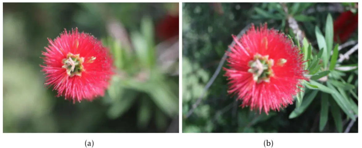
Focus is a key feature in photography as it indicates which parts of the image are sharpest [Cur04]. Naturally, those sharp areas are the ones that draw the most attention from the viewer. It is up to the photographer to decide whether to have a large set of focus points, leading to a globally focused photo or to focus a smaller region in order to emphasize a specific subject in the image. Most photographs have a specific location in the scene which represents their subject. That subject must be where the focus point(s) lie. The focus points of an image are an essential concept in photography for they can change the way an image is perceived by the viewer. For instance, in Figure 2.1 two images targeting the same subject but differing on the focus points are shown, wherein the final result is
(a) (b)
Figure 2.1: Point of focus on the flower petals (a) and point of focus on the flower stalk (b).
2.1.4 Aperture
The aperture is the hole through which light enters the camera [San13]. The wider the aperture the more light is let in. It is measured in f-stops, which is a ratio between the camera focal length and the diameter of the aperture. The f-stop value is conversely opposite to the aperture value, given that the wider the aperture the smaller is the f-stop. Large f-stops are preferable when taking photos where a large depth of field is required such as landscapes. Small f-stops are more suited to take photos where a small depth of field is needed, such as portraits.
2.1.5 Depth of Field
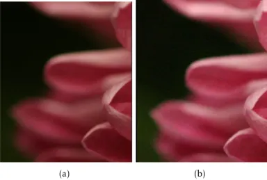
The photographer may control which areas of the image will be focused. Depth of field represents a range of distances at which the objects present in the scene will appear acceptably sharp in the resulting photo [San13]. It depends mainly on the aperture (see Section 2.1.4) and focus length of the camera. Wider apertures (small f-stops) and closer focusing distances origin a shallower depth of field resulting in a local focus effect.
Smaller apertures (larger f-stops) and increased focusing distances result in a deeper depth of field originating a global focus effect, as shown in Figure 2.2.
Regions of objects within the depth of field become less sharp the farther they are from the plane of critical focus [Cur04], as shown in the left side of Figure 2.2. The transition from the sharp region to the unsharp region does not create an abrupt change. The pixels outside the depth of field are not all equally blurred. This phenomenon is commonly referred to as the circle of confusion.
2.1.6 Shutter Speed
C H A P T E R 2 . BAC KG R O U N D & R E L AT E D WO R K
Figure 2.2: Local focus (left side) and global focus (right side)1.
camera sensor to capture the image.
Faster shutter speeds imply smaller exposure times and thus they usually freeze the action in the image. In opposition, slower shutter speeds mean larger exposure times and consequently more light is captured by the camera sensor. A slow shutter speed can create the effect of motion blur that happens when any object moving along the direction
of relative motion appears blurry, as it it shown in Figure 2.3.
(a) (b)
Figure 2.3: Slow shutter speed combined with panning the camera(a); Slow shutter speed but no panning of the camera(b)2.
A negative effect of using a slow shutter speed is to capture an image where most
details are blurred due to camera shake. The slightest move during the exposure, such as trembling of hands or breathing of the photographer or even the simple press of the cam-era shutter button, may result in a blurry image, even if the subject stood still. Figure 2.4
(a) shows the result of an image captured when there was camera motion while (b) shows the expected result.
(a) (b)
Figure 2.4: Blurry image due to camera shake(a); expected result (b)3.
2.1.7 ISO
ISO refers to the level of sensitivity of the camera sensor towards the light by using a numerical scale. The more sensitivity the less time is required to capture the image although sometimes at the expense of grainier images. A lower ISO requires more light in order to create a good exposure. This can be achieved by using a wider aperture or a slower shutter speed. High ISO is preferable when the existing light is scarce. As counterpart, a high ISO will capture a noisy image. The noise influence is shown in Figure 2.5.
(a) (b)
Figure 2.5: Difference between an image with ISO value of 100 (a) and 3200 (b)4.
C H A P T E R 2 . BAC KG R O U N D & R E L AT E D WO R K
Noise is originated because cameras increase the sensitivity by amplifying the signal of the image sensor. The higher the sensitivity increases, the higher the noise in the captured image, as increasing the sensitivity amplifies the captured signal, but also amplifies the background noise captured along with it [Cur04].
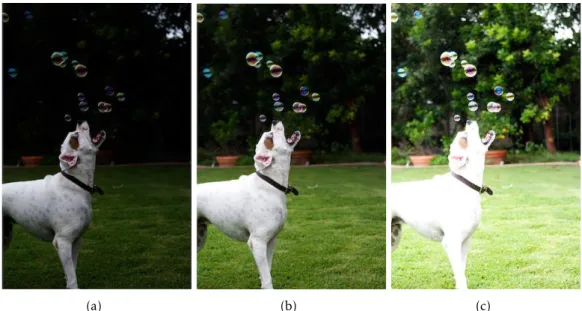
2.1.8 Level of Exposure
The concepts introduced in the sections above, namely the aperture, the shutter speed and the ISO, define the level of exposure in a photo. These three variables are interdependent given that, to keep the same level of exposure, when one of them changes, at least one of the remainder must change too [San13]. The combination of these variables may lead to different types of exposure such as shown in Figure 2.6, where the difference between an
underexposed, a well exposed and an overexposed image is displayed. An underexposed photo is characterized by dark colour tones, an overexposed photo is dominated by bright colour tones while a well exposed photo has balanced lightness in its colours.
(a) (b) (c)
Figure 2.6: Difference between underexposed image (a), the ideal exposure (b) and an
overexposed image (c)5.
2.1.9 White Balance
Looking at the colour spectrum and temperature, it is clear that the colour of light can vary significantly [Fre08]. The human brain can interpret the variance in white light produced by different sources of light making it looknormal. However a camera sensor
captures the light as it is. Thus it is necessary to use white balance in order to match the captured ambient light the way our brain would read it. Figure 2.7 shows an example of an image taken with different tonalities.
Figure 2.7: Top portion iscold. Bottom section iswarm. Middle section shows a correct white balance setting for the image6.
2.2 Image Correlation Algorithms
Image correlation refers to the process of analysing data sets from different images and
to match them in order to enable their comparative analysis. This section is divided in two parts: the first (see Section 2.2.1) approaches the detection of keypoints in images, which are identifiable and peculiar points in the image scope; the second (see Section 2.2.2) refers to how those keypoints, from different images, can be correlated.
2.2.1 Keypoint Detector
Keypoints provide a large amount of information about an image. An important advan-tage of keypoints is that they permit matching even in the presence of clutter (occlusion) and scale or orientation changes. There are multiple feature detector algorithms. In this section the ones considered to provide best results are described: FAST [RD06], SIFT [Low04] and SURF [Bay+08].
2.2.1.1 FAST
Features from Accelerated Segment Test (FAST) [RD06] is a corner detector algorithm best suited to process image features in real-time frame-rate applications due to its per-formance driven implementation. To detect a potential corner an analysis for each pixel
C H A P T E R 2 . BAC KG R O U N D & R E L AT E D WO R K
p in the image is done. Pixelpis a corner if there is a set ofncontiguous pixels in its neighbourhood whose intensities are higher thanI(p) +t or smaller thanI(p)−t, where I(p) represents the intensity value of pixelpandtdefines an appropriate threshold value. Synthesizing, a potential corner is detected if its intensity is distinguishable among the intensities ofnpoints in its neighbourhood. Although FAST is faster than both SIFT (see Section 2.2.1.2) and SURF (see Section 2.2.1.3), it may not perform as good as desirable when images are subjected to variations on scale and illumination.
2.2.1.2 SIFT
Scale-Invariant Feature Transform (SIFT) [Low04] allows the extraction of features that are invariant to image scale and rotation and partially invariant to a substantial range of affine distortions, changes in the 3D viewport, addition of noise and changes in
illumina-tion. It consists of four elemental procedures: keypoint detection, keypoint localization, orientation assignment and keypoint descriptor. Potential keypoints are detected, by a multiscale approach where the image is rescaled, using a Difference-of-Gaussian
func-tion. Afterwards, ambiguous keypoints, i.e., low contrast points, which are not robust to noise, and those that are poorly localized along edges, are eliminated leaving only the stablest keypoints. In the third step, an orientation is assigned to each keypoint based on a histogram computed by the gradient orientation of a sample of points around the key-point. Finally, the standard keypoint descriptor is created by sampling the magnitudes and orientations of the image gradient in the patch around the keypoint and building a smoothed orientation histogram to capture important aspects of the patch.
2.2.1.3 SURF
While SIFT (see Section 2.2.1.2) builds an image pyramid with progressively downsam-pled images, Speed-Up Robust Features (SURF) [Bay+08] uses images with the same resolution but different scaled box filters convolved with the integral image. Potential
keypoints are detected with a Hessian matrix that, according to the authors, presents ad-vantages in terms of speed and accuracy. The dominant orientation is obtained through the Gaussian weighted Haar wavelet response within a circular neighbourhood around the keypoint. Thereafter, a 4x4 oriented quadratic grid is laid over the interest point. For each square, the wavelet responses are computed from 5x5 samples extracting the descriptor from it.
2.2.2 Keypoint Matcher
After obtaining the keypoints of the images, a next logical step is to match them in the different images. Basically, a keypoint matching algorithm will take on the characteristic
properties, such as a keypoint descriptor, detected in images and compare them in order to find similarities. By doing so, it is possible to identify the same subjects in different
2.2.2.1 FLANN
The algorithms described in Section 2.2.1 output a set of keypoints in images. Each keypoint may vary on factors such as the scale where the keypoint was detected and its orientation. Fast Approximate Nearest Neighbor Search (FLANN) [ML09] is a library for processing fast approximate neighbour searches in high dimensional spaces. The main goal of the FLANN library is to analyse data sets, which in this case is a set of keypoints, between different images and then match corresponding elements between different data
sets. Based on the characteristics of the data sets, the most appropriate nearest neighbour searches algorithm is automatically chosen. Beyond the choice of the most appropriate algorithm, the optimal values for the algorithm parameters are also the computed. As for the collection of algorithms to be used, the authors identified algorithms that use hierarchical k-means trees or multiple randomized kd-trees to be the ones that provide the best result in nearest neighbour searches.
2.2.2.2 RANSAC
The result of FLANN [ML09] is a set of matches, i.e. pairs (k1, k2) of nearest neighbours,
wherek1 andk2 belong to different images. However, the appearance of outliers may
occur. An outlier is a false-positive match, where k1 andk2 are matched as being the
same point in different images but in reality they are not. Random Sample Consensus
(RANSAC) [FB81] is an iterative method that analyses a mathematical model, in this case a set of keypoint matches, which may contain outliers. It is a resampling technique that generates candidate solutions by using the minimum number of iterations required to estimate the underlying model parameters [Der10]. For a specific number of iterations, a sample ofnmatches is selected and a homographyHis computed from thosenmatches. Each match is then classified as inlier or outlier depending on its concurrence with H. After all the iterations are done, the iteration that contained the largest number of inliers is selected. Then, H can be recomputed from all the matches that were considered as inliers in that iteration [Dub09].
2.3 Focus Detection Algorithms
Digital images may be analysed in terms of focus. There are different approaches to focus
detection such as analysis based on the spatial domain or a study over the frequency domain. In this section focus detection techniques are presented, as well as some back-ground study for it to be possible.
2.3.1 Fourier Transform
C H A P T E R 2 . BAC KG R O U N D & R E L AT E D WO R K
image spatial domain the procedures are realized directly on the pixels.
Jean-Baptist Joseph Fourier (1768-1830) in his book,The Analytic Theory of Heat[FF78], stated that any function can be expressed as the sum of sines and/or cosines of different
frequencies. Such discovery is important and useful in the branch of image processing as it allows the conversion between the spatial and frequency domains of an image.
The Fourier Transform decomposes an image into sine and cosine components rep-resenting the image frequency domain. When applied on a discrete function, such as digital image, it is commonly referred as the Discrete Fourier Transform (DFT) [GW01]. For an image of sizeMxN, the two-dimensional DFT, which converts the spatial domain into the frequency one, is given by the mathematical expression:
F(u, v) = 1 MN
M−1
X
x=0
N−1
X
y=0
f(x, y)e−j2π(uxM+ vy N)
foru= 0,1,2, ..., M−1 andv= 0,1,2, ..., N−1 wheref(x, y) represents the image in the spatial domain andj is a complex number of value√−1.
2.3.2 Wavelet Transform
The Fourier transform can be a powerful tool to analyse the frequency components of a signal, such as a digital image. However the temporal information is lost in the transfor-mation process.
The wavelet transform takes the temporal information into account making it easier to compress, transmit and analyse images. Unlike the Fourier transform, whose functions are based on sinusoids and thus do not have location, the wavelet transform are based on small waves, called wavelets, of varying frequency and limited duration [GW01]. Thus, it is able to capture both frequency and location (in time) information.
Wavelets became the foundation to an approach called the multiresolution theory. As the name implies, this theory consists in the representation of a function signal in multiple resolutions. Thus, features that cannot be detected in a determined scale may be detected in a different one.
2.3.3 Focus Quality Classification
An appropriate classification of an image focus quality enables the detection of focused regions and allow their distinction from blurred ones. Such analysis can be based on peculiar characteristics of an image [Liu+08] or, another possible approach, is to compare similar images [LY08; Lu+07], namely by their frequency spectra.
wide set of common features with a blurry image, such as low frequency variations, and thus can be computationally interpreted as blurry.
When several similar images are to be processed, there is the advantage of having the ability to compare their frequency spectra. Theoretically, a focused image have higher frequency variations than a blurry one.
Lu et al. [Lu+07] proposed an image fusion method in which they analyse the focus quality of each image pixel by comparing wavelets coefficients of the input image and
a blurred version of itself and then compare the result with the respective pixel result of another image. Supposing that the images to be analysed are f1 andf2, and their
smoothed versions aref1′ andf2′. Df1,Df2,Df1′ andDf2′ represent the high frequency
variations off1, f2,f1′ andf2′, respectively, in their neighbourhood. They conclude the
following:
If a pixel is focused inf1and blurry inf2, then it is more blurry inf2′, i.e
(|Df1−Df2| − |′ Df1−Df2|)≥T
(|Df1−Df2| − |Df1′−Df2|)≥T
If a pixel is focused inf2and blurry inf1, then it is more blurry inf1′, i.e
(|Df1′−Df2| − |Df1−Df2|)≥T
(|Df1−Df2| − |Df1−Df2|′)≥T
If a pixel is focused or blurred both inf1andf2, then
(|Df1−Df2| − |Df1−Df2′|)< T
(|Df1−Df2| − |Df1′−Df2|)< T
WhereT is determined through a genetic algorithm.
Another image fusion method, in which the focus is detected, was proposed by Li and Yang [LY08]. Contrary to the aforementioned method, the method proposed by Li and Yang analyses the image spatial frequency based on regions instead of individual pixels. The first step is the fusion of the input images by pixel-by-pixel averaging. Then the fused image is segmented using a normalized cut technique. By doing so it is possible to segment the input images equally according to the result of the fused image segmentation. After the segmentation process, each region of the image is analysed in terms of spatial frequency, which indicates the overall active level in that region. Considering an image of sizeMxN, whereMrepresents the number of rows andN represents number of columns, the row (RF) and column (CF) frequency variation may be calculated through:
RF= v u t 1 MN
M−1
X
m=0
N−1
X
n=1
[F(m, n)−F(m, n−1)]2
CF= v u t 1 MN
N−1
X
n=0
M−1
X
m=1
C H A P T E R 2 . BAC KG R O U N D & R E L AT E D WO R K
whereF(m, n) is the grayscale pixel value at position (m, n) of the imageF. Hereupon the total spatial frequency (SF) of the image can be defined as:
SF=
q
(RF)2+ (CF)2
By applying the previous computations to each region it is possible to do the compar-ison between respective regions given that the higher is the spatial frequency value the more focused is that region.
2.4 Motion Blur Detection Algorithms
An image may have focused regions and blurred regions. Blur may occur due to an object or an entire region being out of the image depth of field, i.e., out of the volume in which the image is acceptably sharp or it may occur when there is movement in a photographed scene, originating the so called motion blur. This section presents techniques for blur detection and classification as well as relevant background knowledge to that matter.
2.4.1 Image Gradient
The image gradient is a very useful property as it defines directional changes of intensity or colour in an image.
Mathematically, the gradient of a two variable function defines, for each point, a 2D vector taken from the derivatives in the horizontal and vertical directions. For the inten-sity case, the 2D vector points in the direction of the strongest variation of inteninten-sity values wherein the length of the vector corresponds to the rate of variation in that direction.
Computationally, digital images are defined by discrete points so an approximation of the image gradient is computed by convolving the image with a specific kernel. Sobel, Prewitt and Scharr operators are just a few examples of kernels that can compute an image gradient.
2.4.1.1 Sobel Operator
Sobel derivatives have an interesting property since they can be defined to kernels of any size, being constructed quickly and iteratively [BK08].
The Sobel operator computes an approximation of the gradient of an image intensity function combining Gaussian smoothing and differentiation. The directional changes are
computed with the following kernels:
Gx =
−1 0 +1
−2 0 +2
−1 0 +1
Gy =
−1 −2 −1
0 0 0
+1 +2 +1
2.4.1.2 Prewitt Operator
Prewitt presented another operator to compute the gradient of the image intensity func-tion. This operator is composed by the convolution of two filters with the image [BK08].
Unlike Sobel operator, Prewitt does not empathize the pixels that are closer to the center of the mask. The directional changes are computed with the following kernels:
Gx =
−1 0 +1
−1 0 +1
−1 0 +1
Gy =
−1 −1 −1
0 0 0
+1 +1 +1
Where Gx and Gy represent the horizontal and vertical changes respectively.
As refered by Shrivakshan [Shr12] the biggest disadvantage of Sobel (see Section 2.4.1.1) and Prewitt operators is their sensibility to noise, which may lead to a degradation of the gradient vector computation and therefore the appearing of inaccurate results.
2.4.1.3 Scharr Operator
The Scharr operator aims to improve the Sobel (see Section 2.4.1.1) and Prewitt (see Section 2.4.1.2) operators inaccuracy by minimizing errors that occur in the Fourier do-main [BK08]. Convolving the image with small filters, such as a 3x3 filter, may result in output images where the inaccuracy is more notable. Scharr operator tries to surpass this problem by giving more emphasis to the pixels that are closer to the center of the mask.
The directional changes are computed with the following kernels:
Gx =
−3 0 +3
−10 0 +10
−3 0 +3
Gy =
−3 −10 −3
0 0 0
+3 +10 +3
Where Gx and Gy represent the horizontal and vertical changes respectively.
2.4.2 Blur Detection & Classification
A possible approach to blur detection was proposed by Tong et al. [Ton+04]. Their method is based on an analysis over the edge type and sharpness, using Haar Wavelet Trans-form. According to the authors, when blur occurs both the edge type and its sharpness change. They classify edges into Dirac-Structure, Roof-Structure, Astep-Structure and Gstep-Structure. A graphical description of the different types of edges can be seen in
Figure 2.8.
Roof-Structure and Gstep-Structure have a parameterα, (0< α < π/2), which indicates the sharpness of the edge: the largerαis, the sharper the edge is. As the authors state, most natural images are likely to contain all types of edges. When blur occurs, the Dirac-Structure and Astep-Dirac-Structure will disappear while Roof-Dirac-Structure and Gstep-Dirac-Structure tend to lose their sharpness, i.e., theαvalue becomes smaller.
C H A P T E R 2 . BAC KG R O U N D & R E L AT E D WO R K
Figure 2.8: Different edge types [Ton+04].
local maxima (Emaxi) in each scale. Emaxi represents the intensity of the edge, where i = (1,2,3). For a given threshold, ifEmaxi(k, l)> threshold, then (k, l) is labelled as an edge point. An important property of Haar Wavelet Transform is its ability to recover the sharpness of blurred edges: when observed in small scales, the Roof-Structure and Gstep-Structure tend to recover their sharpness. Thus, based on the Emaxi value the determination of whether an image is blurred or not is possible. For any edge point (k, l), this determination is based on five rules:
1. IfEmax1(k, l)> thresholdorEmax2(k, l)> thresholdorEmax3(k, l)> threshold, then
(k, l) is an edge point.
2. If Emax1(k, l) > Emax2(k, l) > Emax3(k, l), then (k, l) is Dirac-Structure or
Astep-Structure.
3. If Emax1(k, l) < Emax2(k, l) < Emax3(k, l), then (k, l) is Roof-Structure or
Gstep-Structure.
4. IfEmax2(k, l)> Emax1(k, l) andEmax2(k, l)> Emax3(k, l), then (k, l) is a Roof-Structure.
5. For any Gstep-Structure or Roof-Structure, ifEmax1(k, l)< threshold, then (k, l) is
more likely to be in a blurred image.
Nedgesrepresents the total number of edge points. IfPer > MinZero, whereMinZerois a positive number close to zero, then the image if assumed to be focused. Otherwise the equationBE=Nbrg/Nrg outputs the blur confidence coefficient for the image.
Other examples of possible approaches to blur detection and classification are based on the image gradient as it offers a great source of information not only in blur detection
but specially in its classification.
Liu et al. [Liu+08] proposed a method for partially blurred images classification and analysis modelled by image colour, gradient and spectrum information. Their system starts by detecting blur and in a second step they classify it. The detection of blurred regions is based on three assumptions:
1. The amplitude spectrum slope of a blurred region tends to be steeper than that of a focused one.
2. Blurred regions rarely contain sharp edges, which result in smaller gradient magni-tudes.
3. Focused regions are likely to have more vivid colours than blurred ones so the max-imum saturation in blurred regions is expected to be smaller than that in focused regions.
Hereupon by analysing the aforementioned features the detection of blurred regions is supposedly accomplished. Their next step is to classify the detected blurred regions. To achieve that they create a smoothed version of the input image, through a Gaussian function, given that:
1. If an image patch is mostly directional-motion blurred, the edges with gradient perpendicular to the blur direction will not be smoothed, leaving strong gradient only along one direction.
2. If an image patch is approximately focal blurred, the gradient magnitudes along all directions are attenuated.
Based on these statements, they construct a directional response histogram for all image patches, where each bin represents a specific direction and the value of that bin denotes the number of pixels which have that direction. Thus, when in face of a motion blurred patch, the histogram presents a distinctive peak in the direction of motion.
Thus, the differentiation between blur is accomplished and it can be classified as
motion blur or out-of-focus blur.
Su et al. [Su+11] proposed another approach to blur classification. Their method is based on a two-layer image composition model, in which each pixelIin an input image is viewed as a linear combination of a foreground colour,F, and a background colour,B, using an alpha mate value. It is defined as follows:
C H A P T E R 2 . BAC KG R O U N D & R E L AT E D WO R K
whereα can be any value in [0,1]. In focused images mostα values are either zero or one. Ifα = 1, pixelI is considered foreground, otherwise it is denoted as background. However, in a blurred image, foreground and background tend to mix together, namely on its boundaries, so α values become decimal as certain pixels are composed by both foreground and background colours.
Hereupon they analyse the alpha channel model constraint, defined by▽α.b∈ {−1,1}, wherebis a vector that denotes the blur extent in horizontal and vertical direction. The blur kernelbof motion blurred images is usually directional, so▽αwill be lines while in an out-of-focus image the▽αwill be spread out at every direction, in a radial manner. Thus by the analysis of the▽α circularity pattern, the distinction between motion blur and out-of-focus blur is achieved.
2.5 Noise Detection Algorithms
Digital noise is usually seen as alienated dots scattered through the image. It is one of the primary factors for image degradation. There are several approaches to noise detection. This section presents filtering-based detection and block-based detection methods.
2.5.1 Filtering-based Detection
The filtering-based approaches, such as the one proposed by Nguyen and Hong [NH12], are done by filtering the noisy input image with a low-pass filter in order to obtain a smoothed version of it. Then, the standard deviation of the difference between the noisy
image and its smoothed version is computed. The process schematic is shown in Figure 2.9.
The insight of this method lies in the fact that low pass filters tend to attenuate the existing noise in an image and so the difference between the noisy image and its smoothed
version will accentuate the noise.
2.5.2 Block-based Detection
Noisy Image
Filter
Noise Estimation
ơ
-+
Figure 2.9: Filtering-based noise estimation schematic.
2.6 Colour Analysis
Colour plays an integral part in image processing as it can provide a powerful descriptor about the information contained in an image. It is known that humans can discern thousands of colour shades and intensities. However they can only differentiate two
dozen shades of gray [GW01]. Such facts are taken into account by the image processing community so that the best results possible can be achieved. This section addresses some important concepts of colour and how they can be analysed, namely by the use of histograms.
2.6.1 Colour Space
Colour space is a specific organization of colours. The RGB is an additive colour space based on the colours ofRed,Green andBlue. A colour in the RGB space is described by how much of each of these components it includes. This is one of the most well known colour spaces as it is used in electronic devices such as televisions, computer screens and digital camera sensors.
C H A P T E R 2 . BAC KG R O U N D & R E L AT E D WO R K
2.6.2 Colour Temperature
Each light source has its own colour, or temperature. Cool colours like blue or violet, defined by smaller wavelengths (400nm-500nm), usually have temperatures between 7000 kelvin to 10000 kelvin. On the other hand, warm colours like red or orange have temperatures from 1000 to 2000 kelvin. In table 2.1, the difference between common
light sources can be seen, in terms of temperature [San13].
Table 2.1: Light sources temperature.
Temperature (Kelvin) Light Source
1000-2000 Candle light
2500-3500 Homemade tungsten lamp
3000-4000 Sunset and sunrise in a clear sky
4000-5000 Fluorescent lamp
5000-5500 Camera flash
5000-6500 Sunlight in a clear sky at noon
6500-8000 Sunlight in a cloudy sky
9000-10000 Sunlight in a heavily cloudy sky
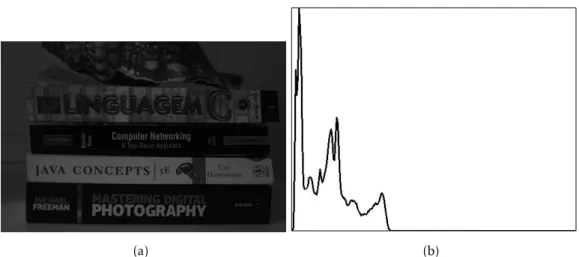
2.6.3 Histogram Processing
A histogram is a graphical representation of how some data values are distributed. In image processing, this is a valuable tool for image evaluation since it allows the analysis of certain image parameters behaviour. For instance, an analysis done on a grayscale image, showing its brightness distribution, can be a hint to distinguish a well exposed image from an underexposed or overexposed one. That is possible because a well exposed image tends to contain a larger range of colours than the other two.
2.7 Photo Quality Estimation
This section presents two similar works [Chu+07; Pot+09] to that presented in this docu-ment. Both works aim at estimating the quality of photos, not necessarily similar, in an album. This estimation is based on technical characteristics such as focus and illumina-tion. Low quality photos are detected and automatically removed from prior processing.
2.7.1 Automatic Photo Selection for Media and Entertainment Applications
In a first step, low quality photos, such as images containing an uneven exposure, blurriness and JPEG artefacts, are detected using machine learning techniques and are not taken into further processing.
Photos affected by compression artefacts, which as stated by the authors looks as
noise, are detected through a filter for deblocking and deriging method [Foi+06]. For adjustment of the filter parameters the top left corner of the square of 3∗3 quantization tableqof the brightness channel is analysed:
k= 1/9
3
X
i,j=1
qi, j
According to the authors experiments, ifkis higher than 6.5 then the photo is consid-ered to be strongly affected by compression artefacts.
Low contrast photos, namely the ones affected by backlighting, are identified from an
analysis over the brightness histogram. The ratio of tones in shadows to midtones and the ratio of the histogram maximum in shadows and the global histogram maximum are two of the values that serve as input to the machine learning algorithm AdaBoost [FS95] in order to detect low contrast photos.
For the identification of blurred photos, each image of the album is convolved with high-pass filters of different sizes. Then an analysis over the variation of the edges is done
over a histogram. The entropy of the histogram characterizes the flatness or peakdness of each histogram. In order for this method to be more effective, the variation between each
image and its smoothed version is also computed. If the variation is high, then the original image is in sharp focus, otherwise it is already blurred. Once again the computations are analysed by the AdaBoost algorithm in order to detect blurred photos.
As a result of the aforementioned approaches, low quality images are removed from further processing. In order to cluster the remaining images, the authors took into con-sideration the moment when the photo was taken and also the camera used to take the photo. That information is obtained through the Exchangeable Image File Format [JEI02] (EXIF). Afterwards, in order to select the best photo from each cluster, they assumed that the most appealing and relevant photo is the most notable one, i.e., the most salient one. Thus, a saliency map is constructed based on intensity, orientation and colour maps being a specific weight applied to each map.
2.7.2 Tiling Slideshow
C H A P T E R 2 . BAC KG R O U N D & R E L AT E D WO R K
of blurred photos, they adopted a wavelet-based method [Ton+04] that analyses edge characteristics at different resolutions, which was already referenced in Section 2.4.2.
Underexposed and overexposed images are detected by comparing the number of dark pixels and bright pixels to a determined threshold. If one of the values surpasses the threshold value then its respective image is considered to underexposed (dark pixels) or overexposed (bright pixels). At this point they claim to have detected the low quality images, so their next step is to group them based on timestamps and content.
2.8 Image Processing Applications
With the advances in photography and technology, the number of image processing ap-plications are constantly increasing. Apap-plications that analyse images from an exposure point of view are no exception. In this section are briefly presented some of those appli-cations, ending with a discussion comparing them and relating them with our work.
2.8.1 Adobe Bridge
Adobe Bridge is a digital asset management application, developed by Adobe Systems[Incc], which may work as a pre-processing unit before editing the photos in Adobe Photoshop. This application offers the option of organizing sets of images in different collections
wherein the user can quickly preview them using a slideshow and also filter them ac-cording to metadata parameters such as the ISO speed, exposure time, focal distance and white balance.
2.8.2 Adobe Lightroom
Adobe Lightroom, developed by Adobe Systems [Incc], lets the user import, organize and create collections of photos and also offering insightful metadata information, such
as histograms. For a comparison between images, the user can choose the compare and survey views, where it is possible to compare pairs of images in more detail, namely by allowing to zoom respective parts of different images and make a visual analysis. However
as the images are not correlated there is still the necessity to navigate in their scope in order to compare respective regions of interest.