Assembly of a portable X-ray fluorescence spectrometer with tri-axial geometry

(1)

Matilde de Jesus Jacob Alves

Licenciada em Ciências da Engenharia Física

Assembly of a portable X-ray fluorescence

spectrometer with tri-axial geometry

Dissertação para obtenção do Grau de Mestre em Engenharia Física

Orientador:

Doutora Sofia Pessanha,

Prof

a

. Auxiliar Convidada,

Universidade NOVA de Lisboa

Co-orientador:

Doutor Mauro Guerra, Prof. Auxiliar Convidado,

Universidade NOVA de Lisboa

Júri:

Presidente: Doutora Maria Isabel Simões Catarino, Universidade NOVA de Lisboa

(2)

(3)

Assembly of a portable X-ray fluorescence spectrometer with tri-axial geometry

Copyright cMatilde de Jesus Jacob Alves, Faculdade de Ciências e Tecnologia, Universi-dade Nova de Lisboa

(4)

(5)

(6)

(7)

Acknowledgements

I would like to extend my gratitude to both of my supervisors, Professor Sofia Pessanha and Professor Mauro Guerra for their effort and support in materializing this project, and for all the learning opportunities they provided me with.

I would like to express my very great appreciation to Professor Maria Luísa Carvalho for her expertise and advice that were so valuable in this project, and for the motivation she always provided.

I would like to offer my special thanks to Dr. João Veloso from the I3N research center of the physics department of the University of Aveiro, for lending us the power supply for the X-ray tube, it was crucial for all the data acquisition present in this thesis.

Furthermore, I would like to express my acknowledgements to Mario Costa, for allowing us to analyze the paper document from his private collection, and that was a fundamental part of this thesis case-studies.

Moreover, the assistance provided by all the colleagues and professors of the lab was also greatly appreciated. I wish to acknowledge the help provided by the Physics Department Workshop for all their work and skills that contributed to the design of this spectrometer. On a more personal level, I would like to thank my family: my mother, Maria Filomena Jacob, and my grandparents, Argemira and António Jacob, for all their love and support throughout all my life and for their encouragement in making me strive for success, I owe it all to you; my boyfriend, Micah Kassner, for his love, patience, and motivation, and for always making me smile.

(8)

(9)

Abstract

X-ray fluorescence (XRF) technique is a powerful analytical tool with a broad range of applications such as quality control, research of environmental contamination by heavy metals, studies regarding cultural heritage, among others.

In this dissertation, a portable energy dispersive X-ray fluorescence (Energy Dispersive X-Ray Fluorescence (EDXRF)) spectrometer will be developed, with orthogonal tri-axial geometry between the X-ray tube, the secondary target, and the sample. Said geometry reduces the background of the obtained spectrum by removing theBremsstrahlungfrom the tube through polarization effects. Moreover, a practically monochromatic excitation energy is obtained. This geometry renders a better peak-background ratio, thus improving the detection limits, leading to superior sensitivity.The use of this geometry has proven to be more advantageous when dealing with the detection of trace elements in low-Z matrix samples. Moreover, the use of a portable setup is of paramount importance in studies related with Cultural Heritage and archaeometry. Thereafter, two case studies will be presented concerning the analysis of a 18th century paper document and the bone remains of an individual buried in the early 19th century.

(10)

(11)

Resumo

A técnica de fluorescência de Raios-X é uma ferramenta analítica poderosa com uma vasta gama de aplicações, tais como controlo de qualidade, pesquisa de contaminação do meio ambiente por elementos pesados, estudos sobre o património cultural, entre outros. Nesta dissertação será desenvolvido um espectrómetro portátil de fluorescência de raios-X dispersivo em energia, com geometria ortogonal tri-axial entre o tubo de raios-X, o alvo secundário, e a amostra. Esta geometria reduz o fundo do espectro obtido através da remoção doBremsstrahlung por efeitos de polarização. Ademais, é obtido um feixe de energia praticamente monocromático. Esta geometria garante uma melhor razão pico-fundo, melhorando deste modo os limites de deteção, o que conduz a uma sensibilidade superior. A utilização desta geometria provou ser mais vantajosa na deteção de elementos traço em amostras constituída por matrizes de baixo número atómico, Z. Além do mais, o uso de uma configuração portátil é de suma importância em estudos relacionados com o património cultural e arqueometria. Consequentemente, dois estudos de caso serão apresentados: a análise de um documento em papel do século 18, e a análise de restos mortais ósseos de um indivíduo enterrado no início do século 19.

(12)

(13)

List of Figures

2.1 Characteristic XRF emission . . . 6

2.2 Auger Effect . . . 8

2.3 Lambert-Beer law schematic representation . . . 8

2.4 Compton Scattering . . . 9

2.5 Schematic representation of incident, reflected and refracted beams . . . 10

2.6 Side-window X-ray tube schematic . . . 13

2.7 Tri-axial Geometry . . . 14

2.8 Spectra assessment . . . 16

3.1 Schematic of an ideal DPP . . . 23

3.2 Cone angle . . . 25

3.3 Secondary target’s support . . . 25

3.4 Detector and supports . . . 28

3.5 Design of the secondary target and collimator support . . . 29

3.6 Secondary target support’s photograph . . . 29

3.7 Setup’s design . . . 29

3.8 Photograph of the setup . . . 30

3.9 Orchard leaves spectra: setup 1 . . . 31

3.12 Photograph of the added lead shielding . . . 32

3.13 Scattering Spectrum . . . 33

5.1 Orchard Leaves Spectrum . . . 38

5.2 Tea Leaves Spectrum . . . 38

5.3 Bush Branches Spectrum . . . 39

5.4 Poplar Leaves Spectrum . . . 39

5.5 Caprine Bone Spectrum . . . 40

5.6 Bovine Bone Spectrum . . . 40

(16)

LIST OFFIGURES

5.8 Bone Ash Spectrum . . . 41

5.9 Winaxilc fitting . . . 42

5.10 Graphic uncertainty calculation . . . 48

5.11 Rib Spectrum . . . 51

5.12 Tibia Spectrum . . . 51

5.13 Femur Spectrum . . . 52

5.14 Photograph of the setup and femur . . . 53

5.15 Document Spectra overlap . . . 55

5.16 Tria-axial XRF set up and paper document . . . 56

5.17 Planar 90oXRF set up and paper document . . . 56

A.1 X-ray tube . . . 66

A.2 X-ray power supply . . . 67

A.3 Detector . . . 68

A.4 Collimator . . . 69

A.5 Collimator’s support . . . 70

A.6 Detector’s support . . . 71

A.7 Inner lead shielding . . . 72

A.8 Secondary target’s support 1/2 . . . 73

A.9 Secondary target’s support 2/2 . . . 74

A.10 Long collimator and secondary target’s acryllic support . . . 75

A.11 X-ray tube’s support . . . 76

A.12 Base support . . . 77

A.13 Long collimator and secondary target’s support . . . 78

(17)

List of Tables

2.1 Electronic levels . . . 15

3.1 X-ray Tube Specifications . . . 22

3.2 X-ray Power Specifications . . . 22

3.3 Secondary Target Thickness . . . 24

3.4 Secondary Target Thickness . . . 24

3.5 Collimators Thickness . . . 26

3.6 Collimators used in the setup . . . 26

3.7 Lead shielding thickness . . . 26

3.8 Bill of Materials . . . 34

5.1 Detection Limits . . . 43

5.2 Detection Limits comparison: portable vs bench top . . . 44

5.3 Detection limit comparison: SSD detector . . . 46

5.4 Accuracy - leaves matrices . . . 49

5.5 Accuracy - bone matrices . . . 49

5.6 Human remains quantification . . . 50

(18)

(19)

List of Acronyms

ADC Analogue-to-Digital Converter.

COPRA Compact Röntgen Analyser.

DAQ Data Acquisition. DL Detection Limits.

DPP Digital Pulse Processor.

EDXRF Energy Dispersive X-Ray Fluorescence. EPD Electronic Personal Dosimeters.

FDA U.S. Food and Drug Administration. FWHM Full Width at Half Maximum Height.

ICP-AES Inductively Coupled Plasma Atomic Emission.

NCRP National Council on Radiation Protection and Measurements. NID Negligible Individual Dose.

NIST National Institute of Standards and Technology.

PIXE Particle Induced X-ray Emission.

ROI Region of Interest.

SDD Silicon Drift Detector.

(20)

(21)

1 Introduction

1.1 Motivation

This thesis purpose is to build a portable X-Ray Fluorescence (XRF) spectrometer with tri-axial geometry in between the X-ray tube, the secondary target and the sample. The XRF technique is a powerful analytical tool with a broad spectrum of applications such as quality control, research of environmental contamination by heavy elements, studies of cultural heritage, and others. Portable XRF spectrometers, in particular, possess an extensive range of applications resulting predominantly from their portability, multi-element capability, fast analysis times, minimal sample preparation requirements, and non-destructive nature [1]. Although the sensitivity of such spectrometers does not come as close as the sensitivity in non-portable laboratory instruments, the implementation of a tri-axial geometry promises an advantageous innovation when compared to other spectrometers of the same sort. Such technology offers a cheap and fast mean of analysis, moreover, it removes the need for sample transportation and storage [1] required in both forensic science and material research in cultural heritage analysis. Concerning the last field of applications, this spectrometer is of the utmost importance for authentication of an assortment of materials, like documents and other pigments materials, and also matching unidentified samples with reference materials (for example, to determine a sample authenticity or historical period) [2].

1.2 State-Of-The-Art

(22)

CHAPTER 1. INTRODUCTION

spectrometric techniques that can be used for portable instrumentation. As formerly de-scribed, there is a need to find a compromise between bench top spectrometer’s high sensitivity and portability regarding XRF spectrometers. In academia and chemical analy-sis market, there is no shortage of portable spectrometers, but there is not yet one merging portability and tri-axial geometry results. Actually, compared to other portable atomic spectrometry techniques, portable XRF has better features like multi-element capability, a less destructive nature, greater simplicity, and more robustness [1]. Considering only portability, the options are numerous, for this is an area that has been evolving through the last decades. There are devices that allowin situsampling and analysis of contaminated soil, like the Spectrace TN 9000 portable P-XRF, and have a better performance when compared to Inductively Coupled Plasma Atomic Emission (ICP-AES). Hence, it remains a useful and fit-for-purpose, powerful tool that provides precise and quick analytic results [4]. Other instruments like compact-XRF Compact Röntgen Analyser (COPRA), allow nondestructive and local analysis of microscopic samples with high elemental sensitivity that can be both used as a bench top unit in a laboratory and a transportable device forin situmeasurements [2]. Also developed in lab was an Silicon Drift Detector (SDD) based XRF spectrometer, whose small size of the detection, excitation module, the elimination of the liquid nitrogen cryostat, and its resolution, makes this device ideal for portable high-resolution XRF spectrometers [5]. Other mobile XRF instrument developed, even though not usually accepted as portable, was focused on the optimization of the glancing angle for a portable total reflection XRF spectrometer. It was concluded that such field portable XRF could provide accurate data and consistent with reference method [6]. Bear-ing in mind only the tri-axial geometry aspect of XRF spectrometers, the options are more limited. Such experimental Energy Dispersive X-ray Fluorescence (EDXRF) spectrometers offer advantages such as simplicity of the associated instrumentation and high efficiency detection system. In this bench top laboratory devices, the X-ray tube, the secondary target and the sample are placed in a tri-axial geometry. Nevertheless, the instrumental design’s simplicity, based in one X-ray tube, a solid state detector and a high voltage generator, does not imply elevated economic costs in the implementation in the industrial process [7]. After studying the role of X-ray reflectivity, coherent, and incoherent scattering in light samples, it was established that the tri-axial geometry is the best geometry for EDXRF apparatus to achieve the best peak-to-background ratio [8, 9]. Comparing two x-ray XRF spectrometers, a portable one and a non-portable one using a metallic Cu alloy as a reference, it was concluded that the detection limits are the main problem of the low-power portable spectrometers, but with more powerful x-ray tubes, the detection limits can be improved [10]. Another evaluation between portable and a stationary XRF spectrometers was performed, regarding scattering radiation for different matrices. It showed similar behavior for both spectrometers, but the portable system presented higher background [10]. Also, the choice of the detectors affects the device’s performance: in a study of detection systems in portable XRF, the Amptek SDD was compared with other two devices, supplanting both. Showing that the fine tuning of the detector parameters

(23)

1.3. GOALS AND WORK STRATEGIES

could improve the overall results for all detectors, and therefore, the general results [11]. Other factors can also improve the instrument’s resolution. For instance, using a capil-lary X-ray lens with a new generation of low power micro-focus X-ray tube and a drift chamber detector enabled a portable unit for micro-XRF with a few tens ofµm lateral resolution in a non-commercial-EDXRF [12]. In another example, an EDXRF was used to analyze different kinds of paper. This technique proved be a good elemental method to differentiate and classify samples [13]. In conclusion, this XRF spectrometer, allied with the engineered tri-axial strategy for ideal portability, all together with a compact design, and high sensitivity makes this instrument a viable alternative to other spectrometers in the market. Furthermore, its success is supported by previously made research, and other spectrometers that were already built and tested.

1.3 Goals and Work strategies

The ultimate goal of this dissertation is to design and build a portable EDXRF spectrometer with a tri-axial geometry, combining the advantages of portability with high sensitivity. To achieve this purpose, the work pursues the following steps:

• Careful planning and design of setup including the choice of materials for the secondary target, collimators, shielding and support pieces.

• Assembling of all the components, testing the existing instrumentation (such as the X-ray tube and detector), and testing different configurations until obtaining the most satisfactory results.

• Spectra acquisition of two groups of standard reference materials, and of two case studies: a paper document and human bone remains.

• Data analysis: detection limits, accuracy and elemental concentration calculations.

(24)

(25)

2 Theoretical Background

2.1 X-ray

This chapter will cover the essential theoretical background of X-ray spectrometry physics. This topic is pertinent to grant an understanding of the core of this dissertation’s basic concepts and focus especially on X-ray emission and production phenomena, as well as in other interaction processes. The X-ray is an electromagnetic radiation that can suffer refraction, reflection, diffraction, and polarization, is not affected by electrical and magnetic fields, and interacts with biological tissues. X-rays’ wavelengths range from 0.01 to 10 nm, consisting in energies ranging approximately from 100 eV to 100 keV. From 5 to 10 keV, the region is named hard X-rays, and the lower energy range is named soft X-rays [14]. Wilhelm Conrad Röntgen is credited as being the discoverer of X-rays in Germany in 1895, and he was the first to systematically study them. Röntgen verified that crystals of barium platinocyanide turned luminescent when there was a discharge from a discharge tube in the vicinity. This occurred with the tube enclosed by black paper, demonstrating that his radiation could penetrate matter. Later, in 1913, Henry Moseley demonstrated that the wavelengths of the spectrum’s lines were characteristic of the element of which the target was made, which led to scientists like Hevesy, Coster, and others, to investigate the potential of fluorescent X-ray spectroscopy as a form of qualitative and quantitative elemental analysis [14]. Currently, X-ray based methods, like X-ray fluorescence spectroscopy, are fundamental in industrial and medical fields and one of the most powerful and flexible techniques available for the analysis and characterization of materials [15]. In the case of this dissertation, XRF will be used in the qualitative and quantitative analysis of constituents of cultural heritage documents and archaeological artifacts.

2.1.1 X-ray Emission

(26)

CHAPTER 2. THEORETICAL BACKGROUND

emission of continuous radiation (Bremsstrahlung), and the emission of characteristic radi-ation.

Characteristic X-rays are emitted from heavy elements when their electrons perform transi-tions between the lower atomic energy levels. If the colliding particle has sufficient energy to remove an orbital electron from the inner electron shell of an atom, the electron from higher energy levels shall occupy the gap, therefore emitting X-ray photons, as seen in figure 2.1.

Figure 2.1: Schematic representation of XRF characteristic emission [16]

Such a process originates an X-ray emission spectrum constituted of spectral lines. These lines of discrete frequencies are also referred to as characteristic lines, for they hinge upon the element used as target. Each of these electronic transitions causes the emission of a photon X. The energy of this X photon is equal to the difference between the binding energy of the final levelsEf, and firstEi:

EX=|Ef −Ei | (2.1)

When high-energy-charged particles lose energy transiting through the Coulomb field of a nucleus, it emits a continuous spectrum of X-ray radiation, also known as

Bremsstrahlung(from the German, meaning “deceleration radiation”). Electromagnetism theory dictates that the emission of radiation from the acceleration of charged particles, hence the deceleration of high energy charged particle penetrating a target must produce radiation. This continuous spectrum is characterized by a short-wavelength limitλ, that corresponds to the maximum energy of the excited electrons [14].

λmin = hc

eV0 (2.2)

Wherehis Planck’s constant,cis the velocity of light, e is the electron charge, andV0

is the applied potential difference.

(27)

2.1. X-RAY

TheBremsstrahlungintensity distribuition is given by:

N(E)dE=kiZEmax E −1

dE (2.3)

Where i is the tube current, Z is the atomic number of the target material, N(E)dE is the number of photons with energies between E and E+dE and k is a constant. This formula, demonstrates that the number of photons is inversely related to the energy E of the photons.

Occasionally, the energy might be first transferred to another electron in an higher shell, and then ejecting it from the atom in order to adjust to a more stable configuration, like in figure 2.2. This spontaneous process is called the Auger effect [17]. The energy of the ejected electron is given by:

Ee =|(Ef −Ei)| −E′ (2.4) BeingEf the energy of the final state andEi the energy of the initial state, and E’ the bonding energy of the level from which the second electron was pulled.

The Auger’s decay competes with the emission of a characteristic X-ray photon and occurs mainly in elements of lower atomic number (Z < 40) [18]. The probability of the Auger effect increases with a decrease in the difference of the corresponding energy states, and it is the highest for low Z elements [14]. If the vacancy is filled by an electron from a higher sub-shell from the same shell, the transition is entitled Coster-Krönig. A consequence of the Auger effect is that the number of X-ray photons produced from an atom is less than expected. The probability of a vacancy in an atomic shell or sub shell giving rise to a radiative transition is called fluorescence yield (ω), or the ratio of the number of X-ray photons emitted to the number of ionized atoms. The fluorescence yield is very low for low Z elements, hence why X-ray spectrometers are less sensitive for lighter elements [19].

2.1.2 X-ray Interaction with Matter

The interaction of radiation with matter depends on the atoms that constitute the material and the energy of the photons. The main processes involving the interaction of radiation with matter, like the photoelectric effect, X-ray scattering and pair production (the latest not being relevant for X-ray for it does not occur for E < 1 MeV [19] ), shall be more thoroughly described in the following subsection.

2.1.2.1 X-ray Attenuation

(28)

Figure 2.2: Schematic representation of Auger effect [16]

of thickness x, the attenuation of the intensity of the beam is described according to the Lambert-Beer law (figure 2.3):

Ix = I0e[−(

µ

ρρx] _(2.5)

whereµ(cm−1₎_{is the linear attenuation coefficient and}µ

ρ (cm2/g) is the mass-attenuation

coefficient for material of densityρ(g/cm3). The intensity exponentially depends on the thickness of the layer. The mass attenuation coefficient (µ_ρ) is a quantity that depends on the composition of the material and the energy of the X-ray photons.

Figure 2.3: Lambert-Beer law Schematic representation for X-ray attenuation [20] For low energies (below 1 MeV) the photoelectric effect is the central interactions of X-rays with matter. This phenomena occurs when a photon with energy equal or greater than the binding energy of the electron interacts with it. The incident photon is absorbed and an electron (photo-electron) is ejected with an energy equal to the difference between the original photon energy and the binding energy [14]:

EX=|Ef −Ei | (2.6)

The probability of the occurrence of such effect is maximum for photon energies in the order of the binding electron energy [18], and it depends onZ4for low energy photons andZ5_{to high energy photons [14].}

(29)

2.1. X-RAY

Abrupt discontinuities in the photoelectric mass absorption coefficient (absorption edges) occur where the energy of the photons become higher than the binding energy of a particular shell [14]

The scattering of X-rays is triggered through two distinct processes: Rayleigh and Compton scattering. The Rayleigh scattering (coherent scattering) - a process by which photons are scattered by strongly bound atomic electrons and in which the atom remains in its ground state. Rayleigh scattering takes place typically at the low energies and for high-Z materials, it’s probability being proportional toZ2_{[14, 21].}

The Compton scattering (incoherent scattering) is the interaction of a photon with a loosely bound outer electron, that translates into a decrease in energy and a change of direction of the incoming photon, thus leading the electron to be ejected in a different direction, as shown in figure 2.4. The conservation of momentum and energy at the collision cause the photon’s loss of energy.

Figure 2.4: Schematic representation of the Compton scattering [22]

The Compton scattering can be described with equation 2.7, in which photon with the energy, E, bounces into another direction with energy, E’, when deflected by an angle,Θ_, while the electron keeps the remaining part of the energy∆_E₌_E₋_E′_:

E′ E =

1 1+ (1−cosΘ₎

E

Ee (2.7)

BeingEethe rest energy of an electron (511 keV).

The geometric setup of the sample, detector and X-ray tube is commonly arranged at 90o, for this is the angle that minimizes the elastic and inelastic scattering into the detector [8]. Regardless of the geometrical effects, the main responsible for diffusion in the matrix of the sample, and the total amount of Compton and Rayleigh scattering.

When added to the photoelectric mass absorption(τ ρ), these effects lead to the total mass attenuation coefficient (equation 2.2):

(30)

Where (σsct

ρ ) is the mass-scatter coefficient (that takes into account both scattering

effects). The mass attenuation coefficient (µ/ρ) is proportional to the total photon interac-tions cross-section per atom according to equation 2.9 [23]:

µ ρ =

σ

NA (2.9)

Where A is the atomic weight (gmol−1),NAthe Avogadro number (6.022×1023atom mol−1_{), and}_σ_{is the sum of the cross-sections for all the elementary scattering and}

absorp-tion processes (barns/atom = 10−24cm2/atom).

Both Compton and Rayleigh scattering processes do not allow the identification of ele-ments by the emission of characteristic radiation after the photoelectric effect. Nonetheless, these processes are accountable for increasing the background in the detector.

2.1.2.2 X-ray Reflection

When radiation crosses media with different refractive indexes it will be deflected from its original track (see figure 2.5), and the relation between the refractive indexes of the medium and the glancing angle is given by Snell’s law:

n1sinθ1 =n2sinθ2 (2.10)

Wheren1,n2are the refractive indexes of each medium.

Figure 2.5: Schematic representation of incident, reflected and refracted beams at the interface of two media [24].

The refractive index can be written as a complex quantity:

n=1₋δ₋iβ (2.11)

where the imaginary,β, is a measure of the attenuation, and 1₋δ, is the real part of the refractive index.Theδvaries with the X-ray energy according to:

δ= Na

2πreρ

Z Aλ

2 _(2.12)

being the imaginary component:

β= λ

4 µ

ρρ (2.13)

(31)

2.1. X-RAY

where (µ/ρ) is the mass attenuation coefficient. In the X-rays region, the value of δ is usually in the order of 10−6, meaning that radiation is weakly refracted by any medium.

When the refraction angle,θr, is 90o_{, the refracted beam will emerge tangentially to the}

surface’s border. Thus, the correspondent angle of incidence is then named critical angle, θcrit:

cosθcrit= n2

n1 (2.14)

When the angle with the interface is inferior to the critical angle, θcrit, the incident beam is totally reflected in the first medium. Sinceθcrit is very small its cosine can be approximated by:

θcrit ≈1− θcrit42

2 (2.15)

If we take into account equation 2.14 and 2.12 and 2.15 :

cosθcrit = 1, 65

E r

Z

Aρ (2.16)

For low-medium atomic number elements,A≈2Zso we have:

cosθcrit= 1, 17

E

√_ρ _(2.17)

Where E is the energy (keV),θcritis the critical angle in degrees, andρthe density, in

g.cm−3.

The reflectivity of a material is given by the intensity ratio of the reflected and incident beam, and it is depending on energy of the beam. The reflectivity can reach 100 % around the critical angle, and it is inferior to 0.1 % for glancing angles of 1oand more degrees.

2.1.3 X-ray Production and Detection

There are several techniques using X-rays aiming to identify the different elements present in a sample. The technique used in this dissertation, X-ray fluorescence, is only one of the many existing techniques that stand out, such as Electron Beam and Particle Induced X-ray Emission (PIXE).

In this dissertation, it was used an X-ray tube to produce X-rays, and its functioning will be described in the upcoming section.

2.1.3.1 X-ray Tube

(32)

Its basic instrumentation usually entails a radiation-shielding, an independent tungsten filament with a current control unit, a high-melting-point metallic anode, a high-voltage connection to the anode, a beryllium foil exit window, and a means of dissipating the produced heat [14]. In order to power the X-ray tube, a controllable, stable high-voltage power supply capable of providing typically between 5 to 60 kV and a low-voltage power supply for providing current to heat the filament are used.

The X-ray tube windows are typically made of beryllium (Be) due to their high trans-mission for low energy X-rays, although, Be windows tend to be very thin (foil thickness in the range of 50 to 250µm [14]), which can lead to fracture [15]. According to the position of the anode and the Be window, we can differentiate reflection and transmission target with side-window (shown in figure 2.6) or end-window X-ray tubes respectively. In the scope of this work, we used a side-window geometry, which is suitable for both high-kV and high-power operation.

Regarding the output of the tube, the maximum intensity of the spectraI′(λ)max corre-sponds to the wave-lengthλ:

I′(λ)max = I′(λImax) (2.18) Being:

λImax = 3

2λmin (2.19)

Bearing in mind the energy-wavelength relation:

E= hc

λ (2.20)

The relation can be written as:

EImin = 2

3Emax (2.21)

The total intensity of the spectra I’ increases with the atomic number (Z) of the anode and the square applied voltage [18]:

I′ =kZV2 (2.22)

k being a constant including the electrons electric current in the tube.

The critical value of voltage corresponds to the situation where the kinetic energy of the electrons is greater than the incident electron binding energy. In this case, there are well defined intense peaks overlapping the continuous spectrum, which constitute the radiation feature element of the anode [25].

(33)

2.1. X-RAY

Figure 2.6: Schematic representation of a side-window X-ray tube [16]

2.1.3.2 Secondary Target and Tri-axial geometry

There are several mechanisms that minimize the background radiation, and it can be done by monocromatizing the maximum excitation radiation. This can be achieved with the use of a filter on the output of the X-ray tube with the appropriate atomic element in order to attenuate the low energy radiation. Another method to monocromatize the radiation is through the use of a secondary target which is excited by the beam of primary X-rays from the X-ray tube and whose characteristic radiation excites the sample. Both of these methods will not entirely monocromatizeKα radiation because the anode line,

theKβ radiation, and high energyBremsstrahlungcontinue to be transmitted, nonetheless,

attenuated.

Another benefit connected with this method is the flexibility of choosing the excitation energy and allowing the detection of elements with low atomic number [14]. The combi-nation of the anode and the secondary target should take into account the compromise between the energy of the X-rays emitted from the anode and the energy necessary to ionize electrons’ shells of the secondary target [18].

Nevertheless, even with these mechanisms, part of theBremsstrahlungis scattered into the detector, which increases the background and decreases the sensitivity of the spectrometer. Hence the need to resort to a tri-axial system.

X-ray radiation can be polarized by scattering [26]. For an unpolarized primary beam, scattering at an angle ofπ/2 results in a nearly complete plane polarization of the scattered X-rays [14, 21]. Through the use of collimators to define the three orthogonal beams, it was shown that signal-to-background ratios were enhanced. When X-ray radiation with energy in the range typically used in XRF, focuses on the secondary target, theBremsstrahlung

(34)

Figure 2.7: Schematic representation of the tri-axial geometry of the XRF spectrometer [28]

2.1.3.3 Collimation

A collimator is a device used to either attain a beam with limited cross section or to produce a beam of parallel rays [29]. In XRF setups, typically the X-rays exit the tube with a conical angular distribution of 100o_{- 150}o_{. In order to reduce the cross section of the}

beam and re-position it, some sort of collimation is necessary [23].

Even though it has the disadvantage of reducing the beam’s intensity, using collimators in a XRF setup narrows the beam to a central active region of the detector, hence diminishing effects such as incomplete charge collection and escape peaks. The collimator’s material should absorb radiation in the range employed energies and should have an easily identi-fiable X-ray spectrum.

In the previous section, it was mentioned that the use of a collimator is of the utmost importance to guarantee the improvement of the signal-to-background radiation, for it enables only the selection of the radiation scattered at a 90oangle (relative to the primary beam). The enhancement of the signal-to-background ratio leads to an increased sensitivity, which allows us to identify trace elements present in the samples that are being analyzed [30, 31].

2.1.3.4 Detectors

The detectors mainly used in energy dispersive X-ray fluorescence are solid-state, high efficiency detectors that support simultaneous multi-elemental analysis, such as Si-PIN and Si-drift detectors SDD, that can be obtained from manufacturers like VortexR _[32],

AmptekR _{[16], Ketek}R _{[33], among others.}

(35)

2.2. SPECTRA

linearity between the incoming photons and the output rate, and proportionality between the pulse and the incoming photon’s energy. Other very important parameters to take into account are the energy resolution, the detection efficiency, and the sensitivity of the detector.

The sensitivity relies on several factors: the intrinsic noise (regulates the quantity of usable signal), the detector window (absorbs some of the incident radiation), and the detector cross-section and volume (calculate the probability of conversion of incident radiation into energy)[23].

The energy resolution measures the ability of the detector to discriminate between photons with very similar energy. This parameter can be indicated as the Full Width at Half Maximum Height (FWHM) of the measured distribution. A greater FWHM indicates a more challenging identification of peaks from photons with similar energies. [34]. The detection efficiency is given by the number of emitted photons that are completely absorbed by the detector [35].

2.2 Spectra

2.2.1 Notation

The characteristic lines in X-ray emission spectra correspond to atomic electronic transi-tions originated from the excitation of the sample. In order to understand the different spectral lines characteristic to the elements, one can use a set of rules: the Siegbahn no-tation [36]. According to this nono-tation, X-ray spectra are classified as K, L, M... (and so on) series, corresponding, respectively, to the atomic levels of the radiative transitions K, L, M, of the emitted photons (see table 2.1). Each series has (2n - 1) transition levels. The K level constitutes the simpler spectra, for it does not decompose in various transition levels. Each one of the series has groups of lines, the more intense group being namedα. As the intensity decreases, the groups are namedβ,γ,δ, etc. Due to the fact that the K and L series are the most intense, these are the best series for elemental characterization and identification, the K being more appropriate for lighter elements, and L for heavier elements and characterizing elements of the sample series [18].

Table 2.1: Some of the common electronic levels with Siegbahn and IUPAC notation [36]. High energy level Low energy level Name of the line IUPAC notation

(36)

2.2.2 Spectra Assessment

In order to assess qualitatively an EDXRF spectrum, one must comprehend the phenomena contributing to the full extension of the spectrum. In the higher energy region, the elastic and inelastic phenomena take over around 90% of the total number of counts.

Figure 2.8: Spectra assessment of the reference sample bone ash, using theWinAxilc

software

We can examine one of the acquired spectra in figure 2.8. The Compton peak’s lower intensity (comparatively with the Rayleigh peak) is due to the sample’s constitution being bone, a heavier Z matrix. The Rayleigh peak has a position and width as expected for a normal fluorescence line. On the other hand, the Compton peak is much broader than a normal characteristic line at that energy. This broader structure is a consequence from scattering over a range of angles and Doppler effect [14].

Other artifacts may be generated throughout the detecting process, the most frequent being the incomplete charge collection, the sum peaks, and the escape peaks.

Sum peaks are a particular form of peak pileup and occur when two X-ray photons arrive to the detector nearly simultaneously and cannot be recognized as separate two events. The pulse, therefore, is measured as the sum of two photon energies [14].

With modern pulse-processing electronics, the pileup effects are mostly suppressed, and the sum peaks are only found when a few large peaks at lower energy dominate the spectrum [14].

Escape peaks are a consequence of the escape of Si-K or Ge-K photons of the detector after photoelectric absorption of the intruding X-ray photon around the edge of the detector. Regarding Si detectors, the escape peak has the energy of the original peak minus 1.74

(37)

2.2. SPECTRA

keV which corresponds to the Kαline energy of Si (for Ge is 9.886 keV). These peaks can

be corrected in a fairly easy way, if one knows the energy, width, and relative intensity of the escape [14].

The incomplete charge collection leads to a measured signal lowered than expected, which is caused when electron-hole pairs generated by an X-ray are not swept to the electrical contacts or when the incident photon does not deposit all of its energy in the crystal [34]. Such phenomena can be diminished by the use of a collimator that prevents the incident radiation from interacting in the edges of the detector [14].

Other artifacts that might be present in the spectrum, are the “forbiden” lines. They corre-spond to the emission of dipolar and quadrupolar magnetic radiation, among others, but they are rather harder to observe, due to their low intensity [15].

All of the phenomena described above lead to the degradation of the signal from the detector and ultimately deteriorate the peak-to-background ratio.

2.2.3 Qualitative and Quantitative Analysis

The qualitative analysis of a X-ray spectrum consists in the identification of each line that constitutes it. Depending on the type of study that is being performed, a qualitative analysis may or may not be enough to obtain the necessary results. In the majority of cases, it is necessary to conduct a quantitative analysis in order to identify and characterize the sample. Quantitative analysis is used to obtain information about the relative amount of elements present in the sample in terms of their concentration (in ppm - parts per million orµg.g−1_).

There are several methods to perform a quantitative analysis, and the method should be chosen accordingly with the application. Considering that the main goal is the de-termination of a single or several elements in an unknown but constant matrix or in a sample with negligible matrix effects, comparative methods should be of choice. If the matrix effects vary within samples and multi-element determination is required, then mathematical methods must be used, such as the influence coefficient correction method and the Fundamental Parameter method [14, 37].

The Fundamental Parameter method is the most commonly used in XRF quantitative analysis. This method allows the calculation of the intensity of fluorescent radiation as a function of the composition of the specimen (weight fractions), the incident spectrum, and the configuration of the spectrometer used. All other variables used are fundamental constants, such as the mass-attenuation coefficients for a given element at a given wave-length, its fluorescence yield and photoionization cross sections [14].

(38)

on the energy of the primary beam and on the elements in the sample, this radiation can generate additional fluorescence in the element, thus enhancing the sample’s signal [18]. Intensity and concentration are related through the following equation:

IPi = I0KimciAi (2.23)

Kibeing the calibration factor,I0is the primary intensity (incident beam), m is sample’s

mass per unit area (g.cm−2) ,ciis the concentration of the element, i, andAithe attenuation factor [38], which is given by [18]:

Ai = 1

+e hµ

ρ(E1,j) sinϕ₁ +

µ ρ(Ei,j)

sinϕ₂

i

m

Σ_j_c_j

hµ

ρ(E1,j) sinϕ1 +

µ ρ(Ei,j) sinϕ2

i m

(2.24)

Σ_j_c_j ₌₁ _(2.25)

whereµ_ρ(E1,j)is the mass attenuation coefficient of the element, j, at the incident energy and µ_ρEi,j is the mass attenuation coefficient for element, j, at characteristic energy for element, i,ϕ1andϕ2are the angles for incoming and emitted radiation from the sample.

The calibration factor,Ki, is:

Ki =ΩεiCi′ωiσXiPL−>_M (2.26) where εi is the efficiency of the detector for element, i, σX_i is the cross section for producing characteristic radiation of an element, i,Ω_{the detector solid angle}_ω_i_{, is the} fluorescent yield for element i, PL−>_M is the transition probability from level L to M in element, i, and C_i′ is the absorption in air and detector window of the characteristic photons of element, i.

If one considers that the attenuation factor does not suffer significant alterations, one can encounter a linear relation between characteristic X-ray line intensity and elemental concentration in equation 2.23. This linear correlation can be attained through matching the matrix of the calibration standards with the unknown specimen under study [39]. This is the foundation for a quantitative method that disregards the matrix effects: the compare method. Due to the nature of the samples used in this dissertation, the compare method is the one that suits better our quantification analysis needs. We will make use of the software packageWinAXILc to perform a fitting and calibration of the spectra and determine the line intensities. Afterwards the calibration lines will be calculated with the OriginLab software and applied to the unknown samples in order to obtain their elemental concentration.

Nonetheless, there are some disadvantages to compare method, the main one being the selection of the calibration standards. This is required to replicate the matrix and the composition of the sample under investigation [21].

(39)

2.2. SPECTRA

2.2.4 Detection Limits, Precision and Accuracy

The suitability of an analytical technique can be measured through its precision, accu-racy, and detection limits for each of the elements for a given kind of matrix. This last parameter stands for the lowest statistically significant concentration level that can be determined from the sample’s analysis. The concentration of each element is calculated through its characteristic peak’s intensity, which involves knowing the average number of total accumulated counts of X-ray photons in a certain Region of Interest (ROI) and the correspondent background counts [40]. Therefore, the EDXRF detection limits (Detection Limits (DL)) can be calculated with the following equation [18]:

DL= 3Ci

√_n

B

nP (2.27)

whereCiis the concentration of the element i,nBis the counting rate for the background andnPis the counting rate for the corresponding peak.

In any scientific method, precision needs to be taken into account. It basically indicates how close the measured values in an experiment are to each other, hence its consistency. Inconsistencies originating from the repetition of the measurements can be due to random errors, which is a type of observational error.

(40)

(41)

3 Experimental Setup

3.1 Instrumentation

In this section, several components of the spectrometer’s setup will be described. The fundamental devices used are the X-ray tube and detector, which will be more thoroughly described in the next sections, but there are other important pieces of instrumentation as well.

In order to perform a dosimetry analysis and guaranty radiation safety around the spec-trometer, a Thermo Scientific Electronic Personal Dosimeters (EPD)-G Dosimeter was used.

Due to the X-ray tube’s high power, when compared to other portable XRF, it’s inner cooling system is not enough to keep the tube and power supply in optimal temperature conditions. For monitoring the X-ray tube’s temperature, a RS Components Digital Ther-mometer was placed on the tube’s surface. To help cool the tube and the tube’s power supply, two Philips desk fans (with 15W) were also used during the spectra acquisition. With regard to control and stabilization of both current and voltage of the tube, a National Instruments Data Acquisition (DAQ) M series (NI USB-621X) was connected to the power supply and managed through a LabVIEW interface. All of the equipment described above was already available at the Physics Department.

3.1.1 X-ray Tube

The X-ray tube used in the experimental set up was a Oxford Instruments Jupiter 5000 Series, designed for applications with high flux and continuous operations, featuring a stainless steal, lead-lined package and filled with dielectric oil to guarantee X-ray shielding and heat dissipation [41]. The most important specifications are shown in table 3.1.

(42)

CHAPTER 3. EXPERIMENTAL SETUP

Table 3.1: Oxford Instruments Jupiter 5000 X-ray Tube Specifications [41] X-ray Tube Specifications

Operating Voltage Range 10-50 kV

Maximum Power 50W

Max. Beam Current 1,0 mA Focal spot size 50µm, 55µm

Window material Be

Window thickness 127µm

Cone of Illumination 23o Window diameter 11,43 mm

Target angle 12o

Max. Operating Temperature 55oC on case surface

Weigh 1,82 kg

Table 3.2: Matsusada Precision X-ray Power Supply Specifications [42] X-ray Power Supply Specifications

Input Voltage 24 V±10%

Power 50 W To 100 W

Output Voltage 0 to 50 kV

Output Current 1 mA

Operating Temperature 0oC to 55oC

Weigh 1,82 kg

The equipment described above was already available at the Physics department of FCT-UNL.

3.1.2 Detector

The detector used is a Vortex-EX silicon drift detector with a 50mm2_{nominal detection}

area, a 500µm thickness and a 12.5µm Be window. The dead layer has a thickness of 100 nm. This detector presents a 133 eV energy resolution at 5.9 keV and 0.25 ms peaking time [11]. The detector is supplied with the electronics box (including a power supply and a digital pulse processor, a vacuum chamber (sealed with a Be window), and the preamplifier box. The Vortex detector package weighs 0.8 kg [43]. This equipment was already available at the Physics department of FCT-UNL, and its technical drawings can be found in Appendix 1, figure A.3.

Generally, the Digital Pulse Processor (DPP) numerically manipulates the signal, usually with the intention to measure, filter, produce, or compress continuous analog signals. The Vortex’s DPP processed result is given by thePI−SpecAc software in the shape of a spectrum. In figure 3.1, a schematic of an ideal DPP is shown, providing information on

(43)

3.2. DESIGN AND MANUFACTURE

the functioning of a DPP. The preamplifier produces an output which consists of small pulses. The said pulses are differentiated so that the step voltage can be measured. A low pass filter improves the signal-to-noise ratio, the output pulses are digitized, and a histogram of the pulse heights is stored in memory. The preamplifier signal is digitized directly using a fast Analogue-to-Digital Converter (ADC). This signal is differentiated using a discrete differencing circuit and sent to a low pass filter which integrates the differentiator output. Afterwards, an algorithm is applied to the input. the digital peak detected is used, and this is value sent to the histogram memory [44].

Figure 3.1: Schematic of an ideal DPP [44]

3.1.3 Software

The software employed to acquire data from the detector was thePI₋SpecAc software. This receives the voltage, current and acquisition time as inputs, and it allows to overlay two different spectra and to save the data in different formats.

Conductive to the fitting of the spectra acquired withPI₋SpecAc , theWinAXILc

was the chosen software. This software grants speed and stability of spectrum analysis, reporting capabilities,and provides a powerful environment for spectrum analysis and manipulation [45]. In section 5.3 there is a more detailed exposition on the fitting process with this software. To quantitatively analyze the acquired data, the softwareOriginLabc

was used. Regarding the design of all the components in this dissertation the software

Autodeskc Inventor was used.

3.2 Design and Manufacture

3.2.1 Secondary Target

The choice of the secondary target is constrained to the energy region we intend to excite, and the fact that the existing X-ray tube has a Mo (molybdenum, Z = 42, EKα = 17,44 keV)

(44)

Considering the X-ray tube’s molybdenum anode, it will emit the following radiation energies (apart from theBremsstrahlungand other lower intensity lines):

Kα Kβ Lα

17,441 keV 19,600 keV 2,293 keV

Given these energies, we were left to choose from Zr (Zirconium, Z = 40, binding energy = 17,99 keV), Y (Yttrium, Z = 39, binding energy = 17,04 keV), Sr (Strontium Z = 38, binding energy = 16,10 keV), Rb ( Rubidium, Z = 37, binding energy = 15,20 keV). Due to unavailability of most materials in a pure, sputtering target format, Y was the final choice, allowing ionization of the Yttrium K-shell with both the Kαand Kβ lines of Mo.

The yttrium target will emit the following X-ray characteristic radiation:

Kα Kβ Lα Lβ1 Lγ1

14,931 keV 16,731 keV 1,922 keV 1,955 keV 2,346 keV

Due to the L lines low energy, they will show in the spectrum in a low energy narrow region (or will not show at all) not relevant for the type of analyses intended with this spectrometer. Hence, the incoming beam that will interact with our samples is mainly formed by yttrium’sKαandKβlines.

Table 3.3: Secondary target thickness calculation ρY[g/cm3] Absorption µm[cm2/g] x[cm]

4,472 99% 10,65 0,096

Table 3.4: Secondary target thickness calculation Binding Energies [keV]

Yttrium [Z=39] Strontium [Z=38] Rubidium [Z=37]

17,04 16,10 15,20

Given the x value from table 3.3 (calculated with Lambert-Beer law and data from the National Institute of Standards and Technology (NIST) [46], an yttrium target (with less than 1 mm thick absorbs 99% of the incident Mo Kαradiation) was purchased from

GoodFellow with the following characteristics:

Purity Thickness Diameter

99% 1,0 mm±15% 25,0 mm±0,5 mm

Concerning the design of the support for the secondary target, the cone of illumination of the x-ray tube must be taken into account to ensure that the entire beam only interacts

(45)

with the secondary target and not it’s surroundings to avoid excitation of elements other than the yttrium.

Figure 3.2: Cone angle [47]

θ =2×tan−1r h

(3.1)

Using equation 3.1, the tube’s provider information about the cone angle, and consid-ering that the tri-axial geometry demands a 45oinclination of the secondary target, we were able to design a proper support. The measures and technical drawing can be found in Appendix 1 (figures A.8 and A.9). Figure 3.3, shows a sketch of the support designed to hold the secondary target in the correct geometry.

Figure 3.3: Two views of the design of the secondary target’s support: technical details in Appendix 1: A.8 and A.9

3.2.2 Collimators

Throughout the data acquisition process, a total of three collimators of two different materials were used. In table 3.6, the sizes and materials of the collimators are shown. Both collimators 1 and 3 had already been purchased by the Physics Department, and collimator 2 was manufactured in the Department’s workshop with silver existent in the lab.

Table 3.5 shows the minimum thickness necessary to absorb 99% of the radiation for each collimator’s material. Comparing with table 3.5, the collimators already existing in the lab met the minimum requirements to be used effectively in this spectrometer.

(46)

Table 3.5: Silver and Tungsten collimators thickness calculation Element ρ[g/cm3] Absorption µm[cm2/g] x[cm]

Ag 10,49 99% 39,98 0,011

W 19,25 99% 138,9 0,002

Table 3.6: Different collimators used in the setup Collimators

Element Internal Diameter [mm] External Diameter [mm] Length [mm] Weight [g]

1 Ag 8±0, 1 10±0, 1 10±0, 1 29,8

2 Ag 2±0, 1 15, 5±0, 1 0, 99±0, 1 2

3 W 2±0, 1 15, 5±0, 1 1, 7±0, 1 6,7

between the secondary target and the sample, and collimator 2 was allocated between the sample and the detector. The technical drawings for collimator 2 and supports for both collimators can be found in Appendix 1, figure A.4.

3.2.3 Lead Shielding

Due to the hazard that X-ray radiation presents for the spectrometer’s operator, there is a need to shield the radiation exiting the tube. This is done through the use of a layer of lead, for this is the best suited material regarding radiation protection. By applying equation 2.5, it is possible to calculate the thickness (x) of the lead shielding necessary to attenuate 99% of the radiation. The results are shown in table 3.7, and a lead shielding tube was built with an approximate thickness of 0,8 mm (thicker than the requirement in table 3.7). In Appendix 1, figure A.7, the technical drawing of the lead shielding is available.

Table 3.7: Lead shielding thickness calculation ρPb[g/cm3] Absorption µm[cm2/g] x[cm]

11,34 99% 14,36 0,028

3.2.4 Dosimetry

During the process of the design of this spectrometer, the undesirable effects of X-ray radiation were taken into account, not only in the spectra itself, but also in the spectrom-eter’s operator. Since continued X-ray exposure can be harmful, dosimetry is needed to study and measure the dose absorbed by ionizing radiation, for monitoring the radiation exposure of individuals, and to design adequate protection.

In dosimetry the mainly used quantity is the absorbed dose, consisting of the energy absorbed per unit mass from any type of ionizing radiation in any target. The previous

(47)

unit of this quantity was the rad, defined as 100 erg.g−1, but currently the gray (Gy) is used, J kg−1[48]:

1Gy≡ 1_kgJ = 10

7_erg

103_g =10 4erg

g =100rad (3.2)

In order to study the effects of radiation on biological tissues and it’s protection, the concept of dose equivalent was created. This quantity (H) is defined as the product of the absorbed dose D and a dimensionless quality factor Q, depending on the linear energy transfer LET, and it’s given by [48]:

H=QD (3.3)

When the dose is expressed in Gy, the (SI) unit of dose equivalent is the rem (“roentgen-equivalent-man”). Since 1 Gy=100 rad, 1 Sv = 100 rem.

Within the scope of radiation protection, a concept that embraces an individual’s exposure to radiation, the Negligible Individual risk level, was delineated . The National Council on Radiation Protection and Measurements (NCRP) defines the Negligible Indi-vidual Dose (NID) without a corresponding risk level, as the effective dose of 0,01 mSv per year [48].

In order to measure the effective dose at the exit of the tube, a calibrated Thermo Scientific dosimeter was placed at approximately 10 cm from the X-ray tube’s exit for the duration of 10 minutes. The obtained value corresponded to 7µSv. Grossly extrapolating this value for the average time of one spectrum acquisition (30 minutes), and considering that for the purpose of this thesis circa 400 spectra were acquired, the total value of the effective dose was 84 mSv. This is a value for extreme conditions, during the acquisition, the tube’s exit is always pointing towards the wall or protected with a 0,8 mm thick lead shield. Besides, the tube has it’s own inner shielding, and the exit towards the secondary target and collimator are also shielded, as described in section 3.2.3. During all of the measurements, the tube was always turned off whenever there was a need to switch the samples. All of these measures minimize the operator’s exposure to radiation, making this device very safe to operate even without external barriers.

According to the U.S. Food and Drug Administration (FDA), the average "effective dose" from natural background radiation is 3 mSv per year in the United States. Regarding diagnostic techniques, the average "effective dose" from a chest X-ray (PA film) is 0.02 mSv, and the effective doses from diagnostic CT procedures are typically estimated to be in the range of 1 to 10 mSv [49], so the total dose from the conditions described above is within the order of magnitude of a CT scan.

(48)

Nonetheless, we would like to perform a more thorough study of the effective dose to which an operator at several distances from the X-ray tube, but, due to equipment constraints, we were not able to performed them.

3.2.5 Other Components

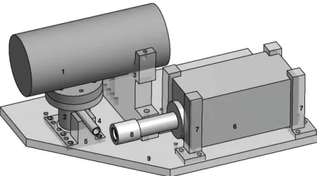
Besides the components described above, other supports were necessary to guarantee the stability of the setup and it’s geometry. Due to the portability of the spectrometer, it is important to have a base with all the components securely attached to it in order to facilitate it’s mobility. A base support for the constituents of the setup was manufactured in acrylic (Appendix 1, figure A.12), as well as a support for the X-ray tube (Appendix A.11) and supports for the detector, shown in figure 3.4 (the corresponding technical drawings can be consulted in Appendix 1, figure A.6).

Figure 3.4: Detector and supports: 1 collimator’s support; 2 acrylic supports; 3 -detector;

To ensure the correct position of the secondary target and the first collimator with the tube, as well as the proper shielding, an aluminum piece was designed in order to align all of these components. Its technical drawing can be consulted in Appendix A, figure A.13. Another acrylic part was design to encompass the aforementioned part and connect it to the setup base support (Appendix 1, figure A.10).

In figures 3.4 and 3.5, it is shown a photograph and a sketch of the designed parts: 1-secondary target support; 2-lead shielding; 3-aluminum support; 4-Silver collimator; 5-Acrylic support.

(49)

Figure 3.5: Design of the secondary target and collimator support

Figure 3.6: Secondary target support’s photograph

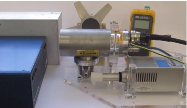
The whole setup assembly can be see in figures 3.6 and 3.7

Figure 3.7: Setup’s design: 1 - X-ray tube; 2 - secondary target’s support; 3 - X-ray tube’s support; 4 Silver collimator; 5 acrylic support; 6 detector; 7 detector’s support; 8

(50)

Figure 3.8: Photograph of the setup, along with the temperature sensor, the cooling fan, the X-ray tube power supply and detector’s power supply and DPP

3.3 Assembly of the Setup

After gathering all the materials and instruments, the setup was assembled as in figures 3.6 and 3.7. Some small adjustments were needed along the process and were done in the department’s workshop. In all of the different setup configurations, the silver collimator (number 1 in table 3.6) was always placed between the secondary target and the sample, and we tested the two other collimators in the nozzle of the detector.

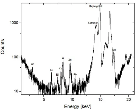
Figure 3.8 shows the resulting spectrum of the orchard leaves (standard reference material NBS-1571) with a tungsten collimator and an aluminum filter (aluminum foil with 0.016 mm thickness) between the secondary target and the silver collimator. Even though the characteristic lines are distinguishable, the peak-background ratio could be improved. In the spectrum, can also be observed molybdenum’s Kαline at 17,44 keV, which should not be observed due to the removal of the radiation coming from the X-ray tube due to polarization. This could mean that the radiation might be entering the detector directly without being doubly polarized by the secondary target and the sample.

In figure 3.9, the aluminum filter was removed from the setup, and the collimator at the entrance of the detector was replaced with a silver collimator (number 2 on table 3.6). Removing the filter lowered the background but did not improve the peak-background ratio. The molybdenum problem remained, and the yttrium’s Rayleigh peak became more intense than the Compton peak, which should not happen due to the low Z of the orchard leaves matrix. This might indicate that the radiation entering the detector was not coming only from the sample’s excitation.

(51)

3.3. ASSEMBLY OF THE SETUP

Figure 3.9: Orchard leaves - Setup: Ag collimator after secondary target, W collimator before the detector and Al filter between secondary target and Ag collimator

(52)

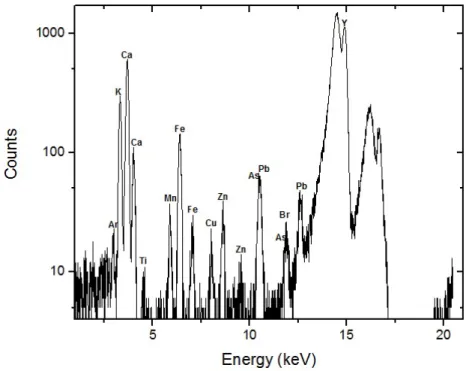
Figure 3.11: Orchard leaves - Setup: Ag collimator after secondary target, Ag collimator before the detector, and extra Pb shielding

Figure 3.12: Photograph of the added layers of lead shielding

To solve the Rayleigh-Compton issue, we tried to adjust the detector’s position, but it was proven that that was not the problem and concluded that non-polarized radiation was coming directly from the tube and exciting the lead in the shielding. This would also explain the molybdenum peak. The most probable cause was the fitting of the collimator tube in the shielding’s hole, and this was fixed by adding another lead shielding in the problem area as shown in figure 3.12.

(53)

3.4. SCATTERING SPECTRUM

The spectrum shown in figure 3.11 was taken after the lead shielding adjustments were made, and the background reduction is very noticeable, as well as the improvement of the peak-background ratio. The Mo characteristic line is no longer present, and the Compton-Rayleigh ratio is compatible with the sample’s low Z matrix.

Henceforward, the setup described above allowed the best results and was the one used throughout the rest of the data acquisition for the samples analyzed in chapter 5.

Shortly after the beginning of the data acquisition with improved setup, the X-ray power supply was broken beyond repair. Fortunately, we were able to borrow the same model of our power supply to finish the measurements within a time constrained period.

3.4 Scattering Spectrum

Initially a diffusion spectrum of a plastic material was acquired to observe the radiation exiting the tube and reaching the sample. One can observe from the diffusion spectra in figure 3.13 that besides the yttrium’s characteristic line (at 14,93 keV), the lead’sLαline (at 10,55 keV) is also noticeable. This is due to the lead barrier that surrounds the X-ray tube’s exit, and it is being excited by the X-rays.

Figure 3.13: Scattering spectrum of plastic

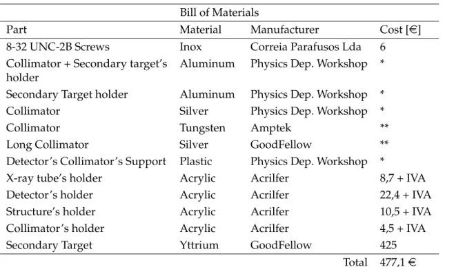
3.5 Bill of Materials

(54)

Table 3.8: Total costs of the materials used to assemble the spectrometer Bill of Materials

Part Material Manufacturer Cost [e_]

8-32 UNC-2B Screws Inox Correia Parafusos Lda 6 Collimator + Secondary target’s

holder

Aluminum Physics Dep. Workshop *

Secondary Target holder Aluminum Physics Dep. Workshop *

Collimator Silver Physics Dep. Workshop *

Collimator Tungsten Amptek **

Long Collimator Silver GoodFellow **

Detector’s Collimator’s Support Plastic Physics Dep. Workshop *

X-ray tube’s holder Acrylic Acrilfer 8,7 + IVA

Detector’s holder Acrylic Acrilfer 22,4 + IVA

Structure’s holder Acrylic Acrilfer 10,5 + IVA

Collimator’s holder Acrylic Acrilfer 4,5 + IVA

Secondary Target Yttrium GoodFellow 425

Total 477,1e

*courtesy of the workshop ** previously purchased

(55)

4 Experimental Procedure

4.1 Samples

With the purpose to test the spectrometer’s potential and to compute it’s detection limits and quantification capabilities, two groups of reference material samples were studied: matrices of leaves(orchard leaves NBS-1571, tea leaves GBW 0765, bush branches GBW 07605, and poplar leaves GBW 07604), and bone matrices (caprine bone NYS RM O5-04, bovine bone NYS RM 05-01, bone meal NIST-1486 and bone ash NIST-1400). The reference materials were available in powder and were processed into pellets to be examined with the spectrometer.

Each sample was pressed into pellets with a 15 mm diameter and 1 mm thick without any chemical treatment. A 10 ton pressure was applied for one minute, and each pellet was glued on a Mylar film on a polyester sample holder. Afterwards, the samples were ready to be examined by the spectrometer.

Besides the standard reference materials, other samples were studied. Human remains from the 18th-19th century were investigated, namely the tibia and ribs. In order to be used in a pellet form, it was first necessary to remove a few grams from the inner compact and trabecular area of the bone, with a polyester tool. Afterwards, the collected bone was powdered in a polyester mill and, only then, pressed into a pellet as described earlier [51].

Within the human remains from this period, a femur was also analyzed. The intention was to have samples sharing the same matrix with the bone matrices reference material in order to establish a quantification.