Analyzing the relationship between the foraging behaviour of two shark species and thermal fronts in the north Atlantic Ocean

(1)

Analyzing the

relationship between

the foraging

behaviour of two

shark species and

thermal fronts in the

north Atlantic Ocean

Inês Gomes Pereira

Recursos Biológicos Aquáticos

Departamento de Biologia 2017

Orientador

Nuno Miguel Cabral Queiroz, Investigador Pós-Doutoral, CIBIO, FCUP

(2)

Todas as correções determinadas pelo júri, e só essas, foram efetuadas.

O Presidente do Júri,

(3)

1

Agradecimentos

Obrigada Doutor Nuno Queiroz por me ter dado a oportunidade de desenvolver este trabalho com o seu grupo, pelos momentos incríveis de descontracção e principalmente pela ajuda nos momentos de maior trabalho.

Obrigada Mestre Ana Couto por teres contribuído tanto para este projecto e pela paciência que tiveste comigo.

Ao Doutor Peter Miller e restantes pessoas que de alguma forma contribuíram para a realização deste trabalho, o meu muito obrigado.

Obrigada à minha família, em especial ao meu pai pelo suporte moral e, sobretudo, pelo incentivo à minha formação e realização pessoal.

Obrigada aos meus amigos pelos momentos de diversão que me enchiam de força, e foram tantos!

Obrigada Filipa Borges por teres um coração tão cheio de bondade.

Obrigada Natalina, o teu espírito jovem é uma inspiração para mim.

Diana, tu és a única coisa indispensável à minha vida. O sentimento que nos une não é traduzido em palavras, apenas existe em nós e apenas nós o podemos sentir. Tudo o que eu faço ou deixo de fazer é em função de ti.

(4)

2 À minha estrelinha polar que mais do que nunca me fez tanta falta, mais do que nunca foi lembrada e amada. Desculpa por tudo o que ficou por desculpar. Agora que cresci reconheço o valor dos teus actos e o amor que estava por detrás deles. É graças a ti que eu sou quem sou e por isso mesmo eu tento amar-me pelas minhas qualidades e pelos meus defeitos, obrigada. “Um amor que é prioritário nunca pode morrer, só pode crescer”, e o nosso amor cresce assim.

A special thank you for all my friends from all over the world! Since I met you, you’ve always kept in touch and gave me support for this great moment of my life. I love you and I’ll never forget you because I brought a peace of each in my heart. People are awaiting us for more solidary actions. Let’s bring more love to this world!

Oumaima, “our souls met before our eyes did”

Este trabalho e todos os anos da minha vida académica são dedicados a vocês.

Henri, my thesis couldn’t start without your amazing version of the Introduction:

“Sharks are cool, they feed in meats because I taste good. We

can study them with negotiation and award them with more meats. The advantages are: we can make them as a cute pet.

Marine fronts are awesome, we can visualize them with battleships and nuclear radar. There might be a relation in terms of world domination and the objective of my study is to

make sure I can be the next queen Elizabeth”.

(5)

3

Resumo

As estratégias de forrageio dos predadores marinhos evoluíram em resposta à distribuição díspar de presas num ambiente vasto, heterogéneo e dinâmico. Essas estratégias permitem que os predadores localizem pontos fortes biológicos, onde a probabilidade de encontrar presas é maior, reduzindo a velocidade e aumentando a taxa de mudança de direcção, de forma a ajustar o esforço de procura em resposta a variações da densidade de presas, o chamado comportamento de procura numa área restrita (PAR), e ao ambiente circundante. Graças às suas características oceanográficas únicas, as frentes oceânicas (gradientes horizontais em propriedades da água, tais como a temperatura, salinidade, entre outras) são ambientes altamente produtivos e consequentemente, pontos fortes de forrageio para muitas espécies marinhas. No entanto, apesar da sua importância como locais de forrageio, o seu valor ecológico para os predadores de topo não é ainda completamente compreendido. Assim, usando mapas frontais compostos de escala fina e dados de rastreio de indivíduos marcados no norte do Atlântico ao longo de 9 anos (2006-2015), pretendemos compreender a influência das alterações dos gradientes térmicos (em frentes oceânicas) no comportamento de forrageio dos tubarões azul (Prionace glauca) e anequim (Isurus oxyrinchus). Mais especificamente, investigamos a relação entre o FPT dos tubarões como uma medida do esforço de procura dos indivíduos, e parâmetros métricos das frentes (intensidade, proximidade e frequência) utilizando Modelos Aditivos Generalizados Mistos (MAGMs). De acordo com os resultados, valores superiores da intensidade das frentes (Fcomp) levam a um aumento da intensidade do comportamento PAR (forrageio) dos tubarões azuis. A mesma relação não foi verificada para os anequins provavelmente porque eu apenas analisei quatro indivíduos com um período de rastreio curto. Também se deveria realizar uma análise em escala mais fina para uma melhor compreensão de como os tubarões se relacionam com as frentes termais. Apesar de não se verificar uma relação significativa para os tubarões anequim, podemos considerar as frentes oceânicas como pontos fortes de forrageio preferidos de disponibilidade aumentada de presas. Esta metodologia tem demonstrado ser útil para estudos das relações entre os movimentos e comportamentos dos animais com o meio ambiente.

Palavras-chave: Rastreio de animais, marcação por satélite, temperatura superficial do mar, esforço de busca, gradientes termais, frentes oceânicas, modelo aditivo generalizado misto, Prionace glauca, Isurus oxyrinchus

(6)

4

Abstract

Foraging strategies of marine predators have evolved to respond to patchy prey distribution in a vast, heterogeneous and dynamic environment. These strategies allow predators to locate biological hotspots, where the probability of prey encounters is higher, reducing travel speed and increasing their turning rates in order to adjust searching effort in response to variations in prey densities, the so-called area-restricted search (ARS) behaviour, and to the surrounding environment. Due to their unique oceanographic characteristics, oceanic fronts (horizontal gradients in water properties, such as temperature, salinity, among others) are highly productive environments and consequently, foraging hotspots for many marine species. However, despite fronts importance as foraging locations, their ecological value for top predators is not yet fully understood. Thus, using fine-scale composite front maps and tracking data from individuals tagged in the north Atlantic over 9 years (2006-2015), I aim to understand the influence of thermal front gradients (in oceanic fronts) on the foraging behaviour of blue (Prionace glauca) and mako (Isurus oxyrinchus) sharks. Specifically, I investigate the relation between sharks’ FPT as measure of individuals’ search effort, and front metrics (intensity, proximity and frequency) using Generalized Additive Mixed Models (GAMMs). According to the results, higher frontal intensity (Fcomp) values lead to an increase in the intensity of ARS (foraging) behaviour in blue sharks. The same relation was not verified for mako sharks, probably because I only analyzed four individuals with a short tracking period. Also a finer-scale analysis should be run in order to better understand how sharks relate to thermal frontal structures. Although no significant relationship was found for mako sharks, we may consider oceanic fronts as preferred foraging hotspots of increased prey availability. This methodology has been shown to be useful for studying links between animal movements and behaviour to the environment.

Key words: animal tracking, satellite-tagging, sea surface temperature, search effort, thermal gradients, oceanic fronts, generalized addictive mixed model, Prionace glauca,

(7)

5

List of Tables

Table Page 1 – Summary data from the 48 individual sharks tagged between 2006 and 2015 in the north Atlantic Ocean; 26

2 – Radii values (m) with the corresponding maximum variance for individual sharks obtained after running the FPT analysis; 61

3 - Summary of model results for blue sharks. Estimated parameters from the final generalized additive mixed model and numerical output for the smoothing function. edf: estimated degrees of freedom; Scale est: estimate scale parameter; R2_{: explanation for} deviance; 33

4 - Summary of model results for mako sharks. Estimated parameters from the final generalized additive mixed model and numerical output for the smoothing function. edf: estimated degrees of freedom; Scale est: estimate scale parameter; R2_{: explanation for} deviance; 33

(10)

8

List of Figures

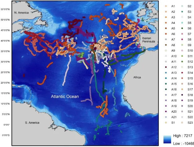
Figure Page 1 - Spatial distributions of satellite-tracked blue sharks Prionace glauca (S1 to S23 and A1 to A21) between 2006 and 2015 in the north Atlantic Ocean; 21

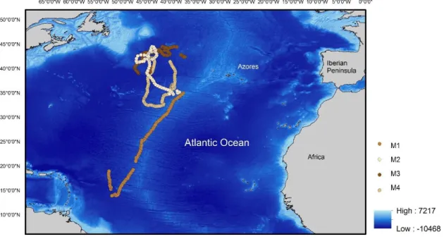
2 - Spatial distributions of satellite-tracked mako sharks Isurus oxyrinchus (M1 to M4) between 2011 and 2014 in the north Atlantic Ocean; 22

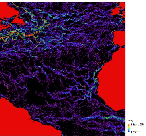
3 - Example of a composite front map with a 7-day window showing thermal fronts in the north Atlantic Ocean (26 June 2010 to 2 July 2010); 24

4 - Example track of shark A14 with (a) the variance in first-passage time for circles of different radius peaking at 824,70 km; (b) first-passage time for each move across an 824,70 km radius circle; and (c) recorded shark positions with the circle of 824,70 km radius.; 29

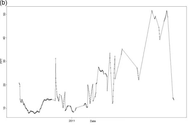
5 - Geographical locations with FPT and correspondent Fcomp of shark S14 (9 June 2014 to 8 January 2015); 31

6 - Geographical locations with FPT and correspondent Fcomp of shark A12 (9 December 2009 to 23 June 2011); 32

7 - Geographical locations with FPT and correspondent Fcomp of mako M2 (10 September to 28 October 2011); 32

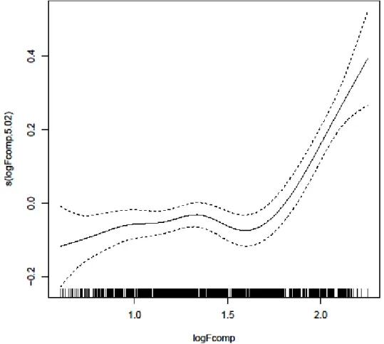
8 - Modelling the relation between Fcomp and FPT with a Generalized Addictive Mixed

Model (GAMM) for blue sharks. Fcomp had a smoothing term significantly different from

zero (p<0.001) and thus contributed to model sharks' FPT. An initial stable relation between FPT and Fcomp was observed, followed by a sharp increase in FPT with the

increase of Fcomp. Dashed lines represent 95% confidence intervals above and below the solid line representing the logFPT. The little vertical lines along the x-axis indicate the FPT values of individual sharks and the y-axis the contribution of the smoother to the fitted values; 34

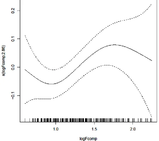
9 - Modelling the relation between Fcomp and FPT with a Generalized Addictive Mixed

Model (GAMM) for mako sharks. GAMM revealed no significant differences in the smoothing term (p>0.001). An initial decrease in FPT is observed, starting to increase around 1.0 with the increasing Fcomp until it reaches a pick and start a smooth decrease.

(11)

9 representing the logFPT. The little vertical lines along the x-axis indicate the FPT values of individual sharks and the y-axis the contribution of the smoother to the fitted values; 35

(12)

10

List of Abbreviations

AVHRR – Advanced very-high-resolution radiometer ARS – Area-restricted search

Chl-a – Chlorophyll a

corAR1 - AR-1 correlation structure

CSIRO – Commonwealth Scientific and Industrial Research Organization CTCRW – Continuous-time correlated random walk

Fcomp – Front composite

FL – Fin length

Fmean – Mean frontal gradient Fpersis – Front persistence

Fprox – Evidence for a feature in proximity

FPT – First-passage time

GAM – Generalized Additive Model

GAMM – Generalized Additive Mixed Model GLS – Global Locations Sensing

GPS – Global Positioning System

IUCN – International Union for the Conservation of Nature lmax - Maximum step length

MAR – Mid-Atlantic Ridge

MODIS – Moderate Resolution Imaging Spectroradiometer PAT / PSAT – Pop-up Satellite Archival tag

Pfront – Probability of observing a front

PFZ – Polar Front Zone

(13)

11 SeaWiFS – Sea-viewing Wide Field-of view Sensor

SIED – Single-image edge detection SPOT – Smart Positions Only tag SST – Sea surface temperature TDR – Time Depth Recorder USA – United States of America UK – United Kingdom

(14)

12

Introduction

Apex predators encompass large pelagic fish species in the top of complex food webs without significant predators except humans. Tunas, swordfish and sharks are examples of apex predators which play a role in structure and stability of marine ecosystem (Myers

et al., 2007; Stevens et al., 2000) through top-down density control of the other species

establishing direct and indirect interactions at multiple trophic levels (Heithaus et al., 2008; Baum & Worm, 2009). Losing top predators can induce trophic cascades and lead dominance of midlevel consumers, modifying all the previous interactions in the environment. (Pace et al., 1999; Worm et al., 2003; Frank et al., 2005).

Overexploitation of fishing resources has been leading to rapid declines of fish communities as well as shark populations worldwide (Shepherd & Myers, 2005; Dulvy et

al., 2008; Ferretti et al., 2010). The high intensity of long-line and other pelagic fisheries

catch many of the same shark species (Bonfil, 1994), which due to their slow growth, late maturity and low reproductive rate have become vulnerable to increased mortality rates (Myers & Worm, 2005).

The knowledge about the ecology of migratory pelagic predators, as the time spent in a given selected area of the sea and its relation with environmental features, allow us to understand their spatiotemporal distribution for the so needed development of conservation and management plans (Block, 2011; Arendt et al., 2012; Kessel et al., 2014; Afonso & Hazin, 2015). Movement ecology is still giving its first steps (Nathan, 2008) and until several years ago, the information on vertical and horizontal movements, habitat preferences and migrations of large marine species were limited. Nowadays there is an urgent need for this kind of information, especially for pelagic sharks (Sims, 2010; Queiroz, 2012).

Species from this study

The species studied here are in danger mainly because of the high catches rates by fisheries: the blue and shortfin mako sharks. The global blue shark population was evaluated as near threatened by the International Union for the Conservation of Nature (IUCN) Red List, probably due to their high catches by long-line fisheries, mainly as by-catch up to 50% of the total by-catch weight (Mandelman et al., 2008; Mejuto et al., 2008). Although they are very abundant and productive than other pelagic sharks (Cortés, 2000;

(15)

13 Frisk, Miller & Fogarty, 2001; Aires-da-Silva & Gallucci, 2007; Anonymous, 2009), there has been a growing concern globally for their conservation.

Because of their high-quality meat and growth in Asian shark fin markets (Dent & Clark, 2015), mako populations had declined since 1986 by commercial and recreational fisheries being the second most heavily caught shark species in the Atlantic Ocean (Cailliet & Bedford, 1983; Hanan et al., 1993; Holts et al., 1998; Camhi et al., 2008) and assessed as Vulnerable by the IUCN Red List.

Still, little is known about the movement ecology of these species. Studies have been limited because of the logistic complications imposed by their oceanic nature, their large-scale horizontal movements, and limits in tracking technology.

Blue shark Prionace glauca

Carcharhinidae is one of the biggest families and comprises the one that is considered the most abundant and best-studied shark species, the blue shark (Prionace glauca Linnaeus, 1758) (Nakano & Stevens, 2008). This large migratory pelagic shark can be found across the globe in tropic, sub-tropic and temperate zones (Compagno, 1984) and has preference for temperatures from 12 to 20ºC, but can tolerate temperatures from 8 to 29,5ºC (Nakano & Nagasawa, 1996). In the Atlantic Ocean their geographic distribution is extensive, making periodic migrations ranging from Newfoundland to Argentina in the west and from Norway to South Africa in the east (Compagno, 1984) and can be found from the surface to 600 m deep (Campana et al., 2011), with the deepest record of 1706 m (Queiroz et al., 2017). Their diet is mainly composed by small pelagic fishes and cephalopods, but it can also include invertebrates, bottom fishes, cetaceans, seabirds and small sharks (Compagno,1984; Clarke et al., 1996; Stevens, 2000; Henderson et al., 2001).

Shortfin mako shark Isurus oxyrinchus

The shortfin mako shark (Isurus oxyrinchus Rafinesque, 1810) belongs to the family Lamnidae and is found in tropical and temperate seas worldwide (Collette & Klein-MacPhee, 2002; Compagno et al., 2005) preferring temperatures from 17 to 22ºC (Compagno, 2001). Like blue sharks, shortfin mako is geographically distributed from Newfoundland to Argentina and from Norway to South Africa in the Atlantic Ocean (Bigelow & Schroeder, 1948; Compagno, 1984) and vertically distributed from the

(16)

14 surface down to at least 500 m depth (Carey et al., 1978). As an apex predator, they feed mainly on teleosts (e.g. bluefish, Pomatomus saltatrix), but also cephalopods, swordfish, marine mammals, sea turtles and other sharks (Mearns et al. 1981; Stillwell & Kohler, 1982; Compagno, 2001; PFMC, 2003).

Telemetry

Ultrasonic telemetry brought the first steps in studying the individual fish behaviour and movements on a small scale (Arnold & Dewar, 2001) with the first publication in 1957 (Trefeden et al., 1957). However, it is not possible to obtain details about vertical and horizontal movements and behaviour over longer time periods.

Static array monitoring was considered by Voegeli et al. (2001) the best available technique for marine fishes. Lowe et al. (2006) used an array of autonomous acoustic receivers to demonstrate whether the tiger sharks (Galeocerdo cuvier), Galapagos sharks (Carcharhinus galapagensis) and Giant trevally (Caranx ignobilis) show affinity to French Frigate Shoals and Midway Atoll from 2000 to 2004. Although the results revealed an effective long-term monitoring of site fidelity and movement patterns of these large marine fishes, some data and also a receiver were lost because of the required maintenance to ensure successful retrieval of data.

Data logging tags were developed in the early 1990s to measure and store large quantities of data and enable vertical and horizontal shark behavioural studies over longer time periods (Sims et al., 2010; Wall et al., 2007). Studies about shark vertical movements have succeeded. However, the horizontal locations are inaccurate because of the absence of transmitters capable of in-air or underwater position finding (Wilson et

al., 1992; Bradshaw et al., 2007). The biggest limitation of archival tags is the physical

recovery by fisheries, mainly because shark recapture is rare and the tag recovering is low (Metcalfe JD & Arnold GP, 1997).

Satellite telemetry has been effective in tracking pelagic air-breathing animals (Mate et

al., 2000; Nichols et al., 2000; Costa et al., 2001), and also animals that regularly come

to the surface, such as sharks (Eckert & Stewart, 2001; Eckert et al., 2002). In the late 1990s, there was the introduction of an electronic tag capable of recording sensor data at a fine temporal resolution over long time periods and with a fishery-independent recovery. Pop-up Satellite Archival tags (PATs or also PSATs) combines an Argos platform transmitter terminal (PTT) to a data-logging sensor. Thus, when detached from

(17)

15 the fish at a pre-programmed date (days/months), it transmits the stored data to the Argos satellite system (Block et al., 1998; Lutcavage et al., 1999). PAT tags can also record depth, ambient water temperature and solar irradiance for estimating the geographic location (Wildlife Computers1_{, 2016). The Argos system uses the Doppler} shift calculations of radio transmissions from the tags (Taillade, 1992) providing accurate latitude and longitude (Wilson et al., 1992).

For horizontal movement studies, the most effective transmitting tags are Argos-linked tags that transmit near-real-time positions every time the animal is above the water, for multiple years and have positioning error under 1 km (Weng et al., 2005). These tags also include a temperature and wet/dry sensor for supporting the transmission of the information about surfacing behaviour and temperature preferences (Wildlife Computers, 2016). These features have advanced studies about a wide range of marine species such as turtles (Hays et al., 2006), seals (Stainiland & Robinson, 2008), tunas (De Metrio

et al., 2005; Stokesbury et al., 2007), billfish (Prince & Goodyear, 2006; Hoolihan & Luo,

2007), swordfish (Neilson et al., 2009) and sharks (Domeier & Nasby-Lucas, 2008; Campana et al., 2009). Such advances in telemetry technology are a key factor in studying animal movement not only in a primarily descriptive way but also quantifying their behaviour and ecological strategies in foraging at different spatial scales.

Area-restricted search (ARS) behaviour

Marine predators are subject to changes in their habitat through different environmental features, such as temperature and light, and their spatial distribution is determined by interactions with other animals, like competitors, predators and prey (Heithaus et al., 2002). They are expected to select prey-rich habitats which generally are patchily distributed in space and time (Fauchald, 1999), thus, spending more time within these high prey density areas when compared to other areas where resources are scarce (Fauchald & Tveraa, 2003). For a successful detection of foraging hotspots, there should be an adaptation of the search behaviour by adjusting its pathway in relation to prey temporal and spatial distribution. In other words, marine predators should reduce their travel speeds and increase their turning rates in order to spend more time in the high-density patches. These adaptations are the so-called area-restricted search (ARS) behaviour (Walsh, 1996; Fauchald, 1999; Farnsworth & Beecham, 1999).

1_{Available at www.wildlifecomputers.com}

(18)

16

First-passage time (FPT) analysis

Novel analytical methods have been used to study scale-dependent movements in animals (Johnson et al., 2002; Fauchald & Tveraa, 2003; Fritz, Saïd & Weimerskirch, 2003; Nams, 2005; Tremblay et al., 2007; Breed et al., 2009) identifying if they are foraging, mating or resting through the tortuosity of the path. A useful indicator of ARS behaviour is the First-passage time (FPT) (Fauchald & Tveraa, 2003) that is, by definition, the time an animal requires to cross a circle of a given radius along its trajectory (Johnson et al., 1992). This circle is moved along the path of the animal at equidistant points, repeatedly with increasing radius. More area of the trajectory is covered by the increasing circle resulting in higher FPT values. The radius that best differentiates between low FPT areas and high FPT areas (transitory areas from intensive search areas) is chosen. It is also expected a higher FPT value in areas with increased sinuosity and/or decreases in movement speed than in areas with faster and more straight-line movements. FPT analysis has been applied in studies to identify ARS behaviour in marine mammals and mostly in seabirds (Thums, Bradshaw & Hindell, 2011; Dragon et al., 2012). Pinaud et al. (2008) showed that FPT analysis can be efficiently used with Argos and GPS as a method for studying animal movement, detecting when the animal changes speed and sinuosity when in contact with a high density of resource, or when the animal reacts to the patch boundary (Benhamou, 1992).

Habitat preference and marine fronts

Environmental factors are often associated with fish diversity and abundance. An interaction between these factors can result in a very important phenomenon known as oceanic fronts. A frontal structure is formed by the meeting of two different water masses creating a convergence at the surface or bottom boundary, which generates a sharp change in the physical parameters, for example temperature and salinity (Largier, 1993), marking physical and chemical boundaries that correspond to biogeographical transition zones (Mann & Lazier, 1991). Such features increase the turbulence, mixing both laterally and vertically, resulting in the input of nutrients which in combination with warm waters (21–24ºC) and sufficient oxygen concentrations (>2 ml l–1_{), enhance biological} productivity (Oschlies & Garçon, 1988; Franks, 1992; Yoder et al., 1994; Acha et al. 2004; Worm et al., 2005). These conditions determine prey distribution and consequently allocate a high diversity of open-ocean top predators to oceanic fronts (Worm et al. 2003, 2005; Vlietstra, 2005; Boyce et al., 2008) where they find favorable feeding conditions. Some studies found it in seabirds (Guinet et al., 1997; Hamer et al., 2009, De Monte,

(19)

17 2012), marine mammals (Bost et al., 2009; Field et al., 2001; Scales, 2014b), turtles (Chambault et al., 2015) and fishes like tunas (Fiedler & Bernard, 1987; Royer et al., 2004), swordfish (Podesta et al., 1993) and sharks (Sims & Quayle, 1998; Etnoyer et al., 2004; Priede & Miller, 2009).

Marine fronts are known attraction areas for sharks in all oceans. For example, porbeagle sharks (Lamna nasus) aggregate along marine fronts of the northwest Atlantic during spring (Campana and Joyce, 2004); salmon sharks (Lamna ditropis) revealed more ARS behaviour when migrating in the highly productive Subarctic Alaska Gyre than those that migrated to the low productive Subtropical Gyre (Weng et al., 2008); whale shark occurrence was significantly influenced by sea surface temperature (SST) and strong thermal gradients, indicating that whale sharks spent more time in frontal regions associated with upwelling systems in the Gulf of California, Mexico (Ramírez-Macías et

al., 2017).

The Atlantic current system, among many other factors, is known to influence the distribution of blue sharks (Stevens, 1990; Kohler & Turner, 2008). Queiroz et al. (2012) tracked blue sharks in the northeast Atlantic in order to determine their vertical niche and horizontal movements and if it is influenced by oceanographic features. Sharks were tagged with PAT tags between July 2006 and June 2008 in the English Channel off south-west England and off southern Portugal. In general, all sharks moved south-west from the tagging sites, with only one shark remaining in the continental shelf dominated by the presence of tidal fronts. It was evident a site fidelity to localized high-productive regions where fronts were present, for example, one shark displayed an initial southward movement towards the African coast and continued to move south reaching the Western Sahara upwelling system in mid-July 2008. Blue sharks spent more time near the surface during the day and night, but displayed a distinct normal diel component in maximum depth, repeatedly displayed during the day below the thermocline (~100m), most probably for feeding, while diving above the thermocline during night hours.

A study was carried about shortfin mako shark in the western north Atlantic Ocean off the coast of the northeastern United States of America (USA) and the Gulf of Mexico for a detailed investigation on vertical movements included in the context of horizontal movements (Vaudo et al., 2016). Eight sharks were tagged between 2004 and 2012 with PAT tags. Vertical movements were strongly associated with ocean temperature, with a narrow distribution of shallow depth in cooler bodies of water and a greater range of depths in the warmer ones. Two sharks were tracked for several months in the western

(20)

18 north Atlantic and moved southerly, leaving the region of the continental shelf during the autumn and showing seasonal horizontal movements from cooler to warmer waters. The other three sharks tagged in this region remained over the continental shelf. The two sharks tagged in the mouth of the Gulf of Mexico traveled northeast into the deeper waters between Campeche Bank and West Florida Shelf. Then, they took different directions with one shark moving to the northern Gulf of Mexico and the other shark moving to the southwestern Gulf of Mexico. In similarity, Block et al. (2011) reported the same movement, from cooler water to warmer water, in the eastern north Pacific Ocean associated with seasonal changes in water temperature and productivity, and in the southeastern Indian Ocean where Rogers et al. (2015) observed northward movements.

Thermal fronts visualization

The analysis of oceanographic features has been based on some important environmental predictors as SST and chlorophyll a (chl-a) that play a significant role in species richness patterns due to optimal thermal ranges and food availability (Etnoyer et

al., 2004; Worm et al., 2005; Mitchell et al., 2014). However, there is some concern about

the capacity of these traditional measurements for predicting distributions of marine predators (Burger, 2003; Grémillet, 2008) because visible and infrared satellite data are severely affected by cloud cover. Recently, the composite front mapping (Miller, 2009; Miller & Christodoulou, 2014; Scales et al., 2015) was developed to identify discrete oceanographic frontal features by combining the locations of frontal fragments derived from all clear sea patches in a sequence of satellite images with full resolution of dynamic features that are not blurred. Simplifying this, composite front maps result from the combination of all fronts detected on a sequence of images from few days into a single map, with the information about location, strength and persistence. Full methodology can be found in Miller (2009).

An example of how this approach can be effective on the characterization of frontal activity is the study carried by Miller et al. (2015). In this study, seven basking sharks were tracked with PAT tags off north-west Scotland and south-west England between May and August in 2001 and 2002, in combination with high-resolution composite front mapping (1 km pixel size; 7-day composites; Miller, 2009) to investigate levels of association with fronts occurring over two spatiotemporal scales (broad-scale, seasonally persistent frontal zones and contemporaneous thermal and chl-a fronts). The tracked sharks were more likely to be found in association with seasonally persistent

(21)

19 frontal zones and their habitat selection was more influenced by contemporaneous mesoscale thermal and chl-a fronts. Seasonal front frequency metrics were significant predictors of shark presence, both over seasonal timescales and in near real-time, in frontal activity and indicated that sharks may return to spatiotemporally predictable foraging grounds where they foraged previously.

Objectives

Despite fronts’ importance as foraging locations, their ecological value for top predators is not yet fully understood, mainly because the majority of them has low population abundance, which makes difficult to get sufficient data to support studies aiming to understand the relation between movements and behaviour with the environment (Pade

et al., 2009). Thus, using fine-scale composite front maps and tracking data from

individuals tagged in the north Atlantic over 9 years (2006-2015), I aim to understand the influence of frontal activity on blue and mako sharks’ foraging behaviour. Specifically, I will investigate the relation between sharks’ FPT as a measure of individuals’ search effort, and front metrics (intensity, proximity and frequency) using Generalized Additive Mixed Models (GAMMs). This study will provide novel information on the spatial and temporal distribution of two top predators, providing the basis for the development and establishment of adequate management and conservation strategies.

(22)

20

Materials and Methods

Shark tagging

I used tracking data from 48 individuals from two different shark species, the blue (Prionace glauca) and shortfin mako (Isurus oxyrinchus). Capture and tagging methodology are fully described in Queiroz et al. (2016) and Vandeperre et al. (2014). Sharks were tagged in three different regions, in the north-eastern Atlantic (off southern England and mainland Portugal), north-western Atlantic and mid-Atlantic in the Azores archipelago.

A total of 12 blue (S1 to S12) and 2 mako (M1 and M2) sharks were tagged between 2006 and 2011 with SPOT tags (SPOT5, Wildlife Computers, Redmond, WA, USA) attached to the first dorsal fin with stainless steel bolts, neoprene and steel washers, and steel screw-lock nuts. A total of 11 blue (S13 to S23) and 2 mako (M3 and M4) sharks were tagged with KiwiSat 202 PPTs (Sirtrack, New Zealand) between 2014 and 2015 following the same methodology.

The remaining 21 blue sharks (A1 to A21) were tagged off an auxiliary 7 m, low gunnel, fiberglass boat, at the surface after immobilization and induction of tonic immobility (Meyer et al., 2010), between 2009 and 2012 in the Azores archipelago. SPOT tags were attached to the dorsal fin of sharks measuring 127 to 211 cm Fork Length (FL) through four nylon threaded rods fixed through stainless steel nuts. Three females (A4, A5 and A6) were double tagged with SPOT and PAT tags (MK10-PAT, Wildlife Computers, Redmond, WA, USA) measuring 142 to 175 cm FL. All tags were pre-programmed to detach from the shark after a period of days.

Track reconstruction

Track reconstruction of both blue and mako sharks are described in detail in Queiroz (2016). Geographical positions of SPOT and KiwiSat 202 tags’ transmissions were obtained through the Argos system. Argos calculates locations by measuring the Doppler Effect on transmission frequency and provides different LCs (LC 3, 2, 1, 0, A, B and Z) based on error calculation (Argos User’s Manual2_{). The tracks were interpolated in order} to obtain daily positions. The LC data were analyzed point-to-point with a 3 m·s-1 _speed filter. The raw Argos locations were processed with a Continuous-time correlated random walk (CTCRW) space model producing the animal daily positions. CTCRW

(23)

21 space model couples a mechanistic model of movement to the data and inferences of the animal positions can be made. Locations are based on the probability of presence at a certain point given its current state (Patterson et al., 2008). These Argos positions were parameterized with the K error model parameters for longitude and latitude using “crawl” package in R (R Core Team, 2016). Figure 1 and 2 show the spatial distributions of blue and mako sharks, respectively.

Fig. 1 – Spatial distributions of satellite-tracked blue sharks Prionace glauca (S1 to S23 and A1 to A21) between 2006 and 2015 in the north Atlantic Ocean.

(24)

22

Fig. 2 - Spatial distributions of satellite-tracked mako sharks Isurus oxyrinchus (M1 to M4) between 2011 and 2014 in the north Atlantic Ocean.

FPT analysis

The FPT analysis were performed using the fpt function of the “adehabitatLT” package in R v.0.99.892 (Fauchald & Tveraa, 2003; R Core Team, 2016) for sharks’ search effort quantifications. We split the track in sections to find the maximum step length (lmax) of each part and set the maximum of distance traveled between sections as the maximum radius r. After this, FPT values were calculated by moving the circle at variable distance for spatial scales r from 25 km (0.04 km to 2*lmax) at increments of 0.10*lmax (Bradshaw

et al., 2007). FPT is found by measuring the time lag between the first crossing of the

circle backward and forward along the path (removing the first and final points of the track where the FPT is unknown) with higher values for more intensively searched areas. FPT is a scale-dependent measure of sharks’ search effort, so that the ARS scales were determined by the value of r with the maximum variance in the log-transformed FPT values to ensure the variance is independent of the magnitude of the mean FPT (var[log (FPT)]). Thus, for each individual track, I plotted the logFPT against r and identified peaks in variance. By the analysis, I was able to locate where sharks showed more intense foraging behaviour during their tracking period (Fauchald & Tveraa, 2003).

(25)

23

Composite front mapping

In order to create a composite front map, some parameters need to be calculated. Single-image edge detection (SIED) algorithm (Cayula & Cornillon,1992) is used for processing SST scenes within 7-day window from Advanced very-high-resolution radiometer (AVHRR) and Sea-viewing Wide Field-of-view Sensor (SeaWiFS) data with a temperature difference threshold of at least 0.4°C (conversion of raw satellite data into calibrated ocean temperature and colour products is summarized in Appendix A in Miller, 2009). The composite duration appears to be long enough to provide the multiple observation of the most genuine features, and not too long that features are obscured by multiple adjacent observations (Miller, 2009). An example of a composite front map can be seen in figure 3. The short-period composites were used in this study because I aim to examine dynamic features instead of static features, which were examined in past studies using composites of weeks or months (e.g. Ullman & Cornillon, 1999), and also because long-period composites can mask neighboring features (Miller, 2009).

The processed SST are then composited to calculate the mean frontal gradient map

Fmean derived from the sequence of front maps, the probability of observing a front at a particular pixel during the sequence Pfront and the evidence for a feature in proximity Fprox. With this information, the front persistence Fpersist, that is defined both by the gradient and the frequency a front is observed at the same location, can be calculated. On a final stage, the front composite Fcomp map is generated by combining all the previously

referred parameters and provide a better visualization of the oceanic features (Miller, 2009, 2016). Figure 3 show an example of a composite front map.

Using fine-scale SST composite front maps I obtained information on front metrics for each shark tracking period by calculating the mean Fcomp using Cell statistics from the Local toolset in ArcGIS, which calculates the mean per-cell from multiple rasters, in other words, it gives the mean raster calculated from the rasters correspondent to a shark tracking period. The raster value for each point of the tracks was also calculated using

Extract value to points from the Extract toolset in ArcGIS, which extracts the cell values

of a raster based on a set of point features. Raster values were recorded in the attribute table of an output feature class and used in further analysis.

(26)

24

Fig. 3 – Example of a composite front map with a 7-day window showing thermal fronts in the north Atlantic Ocean (26 June 2010 to 2 July 2010).

GAMM design

To analyze the spatial relationship between Fcomp and FPT, a GAMM was applied

separately for each of the species using the “mgcv” package in R (Wood, 2006; Zuur et

al., 2009; R Core Team, 2016).

GAMMs are an extension of Generalized Additive Models (GAMs) (Hastie & Tibshirani, 1990) incorporating a smooth interaction of space and time with some of the predictors being treated as random factors. They allow for nonlinear responses in the data and their use have been proposed for studies where there are differences in measured parameters for different individuals (Stroud et al., 2001; Gelfand et al., 2005; Strickland et al., 2011). In each model, individual sharks (ID) was treated as a random factor while the log-transformed Fcomp and FPT were set as fixed effect variables. Instead of treating the data as a single individual I want the model to treat each individual shark as a unique time series, that is why I use shark (ID) as a random factor. The logFPT was set as the response (or dependent) variable while logFcomp was set as the explanatory (or independent) variable. Variable logFcomp was modeled using a smoothing function

(27)

25 estimated by thin-plate regression spline. The optimal amount of smoothing was automatically estimated using cross-validation (Wood, 2006). An auto-regressive process of order 1 (corAR1) was added to allow the temporal autocorrelation in the dataset. For example, it assumes that a track position at time t is dependent on the magnitude of the position at time t-1 (Zuur et al., 2009). Our final formula was:

logFPT ~ s(logFcomp)

The 95% Bayesian confidence intervals were estimated following Wood (2006). Model validation and all the previously mentioned steps were performed following Zuur et al. (2009) in R (Core Team, 2016).

(28)

26

Results

The 48 individuals resulted in 8429 d of tracking data and an average trip duration of 175,60 d. In general, blue and mako sharks displayed a broad distribution among the different north Atlantic regions. The majority of the individuals were oceanic, with exception of sharks S2-S4 that remained in the south-west England, and sharks S5, S7, S9, S10 and S13 that did not leave the southern Portugal area. The longest deployment registered was from a female (A6) that traveled an estimated 28139 km over a 952 d tracking period and the shortest deployment was from the female S5 that only traveled 113 km during 23 d. Blue sharks tagged in Azores displayed extensive movements, with the female A14 traveling straight to the south and reaching the southern hemisphere. Eight individuals (four females and four males) were tracked for over a year (A1, A2, A6, A12, A14, A17, A20 and A21) allowing the observation of a full season cycle. Only the mako M1 moved southeast and had the longest tracking period among mako sharks. Distribution patterns tended to be more northwest in summer while it was more south-easterly in winter for both species. Table 1 summarizes the information about all the individuals used in this study.

Table 1 – Summary data from the 48 individual sharks tagged between 2006 and 2015 in the north Atlantic Ocean.

Name Species Size

(cm FL) Sex Location tagged Tag Tagging date Days-at-liberty Distance (km) M1 Isurus

oxyrinchus 210 F Oceanic SPOT 5

5 Sep

2011 58 3773 M2 Isurus

oxyrinchus 200 M Oceanic SPOT 5

8 Sep 2011 50 3849 M3 Isurus oxyrinchus 185 F Oceanic KiwiSat 202 13 Aug 2015 32 3372 M4 Isurus oxyrinchus 180 M Oceanic KiwiSat 202 9 Jun 2014 23 3455 S1 Prionace

glauca 210 F Oceanic SPOT 5

29 Aug

2011 46 750 S2 Prionace

glauca 186 F England SPOT 5

15 Aug

2006 8 231 S3 Prionace

glauca 170 F England SPOT 5

18 Aug

2006 14 302 S4 Prionace _glauca 160 F England SPOT 5 31 Aug ₂₀₀₆ 21 525 S5 Prionace

glauca 145 F Portugal SPOT 5

1 Jun

(29)

27

S6 Prionace

glauca 220 M Portugal SPOT 5

2 Jun

2009 102 3379 S7 Prionace

10 Oct

2006 23 173 S8 Prionace

6 Jun

2008 101 157 S9 Prionace

17 Jun

2008 112 835 S10 Prionace

26 May

2009 12 254 S11 Prionace

30 Aug

2011 18 510 S12 Prionace

2 Sep 2011 33 969 S13 Prionace glauca 120 F Portugal KiwiSat 202 20 May 2015 39 558 S14 Prionace glauca 205 M Oceanic KiwiSat 202 9 Jun 2014 213 8968 S15 Prionace glauca 145 F Oceanic KiwiSat 202 12 Jun 2014 225 10070 S16 Prionace glauca 220 F Oceanic KiwiSat 202 5 Jun 2014 407 1487 S17 Prionace glauca 220 F Oceanic KiwiSat 202 5 Jun 2014 93 3394 S18 Prionace glauca 230 F Oceanic KiwiSat 202 5 Jun 2014 10 525 S19 Prionace _glauca 215 F Oceanic KiwiSat ₂₀₂ 14 Jun ₂₀₁₄ 20 655 S20 Prionace glauca 210 F Oceanic KiwiSat 202 7 Jun 2014 15 767 S21 Prionace glauca 190 F Oceanic KiwiSat 202 7 Jun 2014 10 479 S22 Prionace glauca 220 F Oceanic KiwiSat 202 9 Jun 2014 56 769 S23 Prionace glauca 220 F Oceanic KiwiSat 202 11 Jun 2014 42 1560 A1 Prionace _glauca 127 F Azores SPOT 19 Feb ₂₀₀₉ 877 14494 A2 Prionace

glauca 139 F Azores SPOT

19 Feb

(30)

28

A3 Prionace

26 Feb

2009 90 2637 A4 Prionace

glauca 175 F Azores Double

26 Aug

2010 226 8275 A5 Prionace

26 Aug

2010 30 911 A6 Prionace

26 Aug

2010 952 28139 A7 Prionace

glauca 130 M Azores SPOT

2 Dec

2009 42 973 A8 Prionace

16 Oct

2009 36 1213 A9 Prionace

16 Oct

2009 206 5041 A10 Prionace

16 Oct

2009 161 5108 A11 Prionace

2 Dec

2009 82 2245 A12 Prionace

20 Aug

2010 579 15498 A13 Prionace

20 Aug

2010 244 6892 A14 Prionace

20 Aug

2010 381 13066 A15 Prionace

20 Aug

2010 126 2364 A16 Prionace _glauca 183 M Azores SPOT 20 Aug ₂₀₁₀ 116 3846 A17 Prionace

20 Aug

2010 524 15066 A18 Prionace

20 Aug

2010 212 5994 A19 Prionace

20 Aug

2010 228 6710 A20 Prionace

20 Aug

2010 369 12451 A21 Prionace _glauca 211 M Azores SPOT 20 Aug ₂₀₁₀ 526 14500

(31)

29

FPT analysis

I performed FPT analysis to quantify sharks’ search effort. Peaks in varFPT/area were observed for all the individuals (Table 2, Annexes), with maximum variance values ranging from 0.04 to 2.49 and FPT radius between 25.00 and 824.70 km. For mako sharks, the FPT radius ranged from 58.00 to 268.55 km, while for blue sharks (S1-S23) the FPT radius ranged from 25.00 to 604.64 km. Blue sharks tagged in the Azores (A1-A21) had the greatest range with FPT radius from 25.00 to 824.70 km. In Figure 4 we can see an example of the resultant plots for shark A14 after running the FPT analysis.

(32)

30

Fig. 4 – Example track of shark A14 with (a) the variance in first-passage time for circles of different radius peaking at 824,70 km; (b) first-passage time for each move across an 824,70 km radius circle; and (c) recorded shark positions with the circle of 824,70 km radius.

(33)

31

Composite front maps

In order to understand how the gradients of SST in the north Atlantic relates to individual shark distribution patterns, composite front maps were generated for each individual for their entire tracking period. Associations of individual sharks with the respective composite front map showed a preference for highly productive areas such as the Gulf Stream, North Atlantic Current, Azores islands, Mid-Atlantic Ridge (MAR) southwest of the Azores and the Iberian Peninsula. This site fidelity is evident for some individuals, for example, shark S14 tagged in the Mid-Atlantic moved to the Gulf Stream in the beginning of August until mid-November (Figure 5).

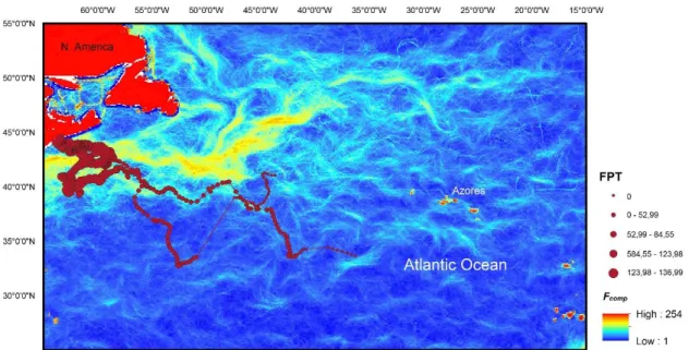
Fig. 5 – Geographical locations with FPT and correspondent Fcomp of shark S14 (9 June 2014 to 8 January 2015). Shark A12 tagged in Azores spent the winter in this region and then moved northward exploring the Gulf Stream in east and south of the Flemish cap during summer. About seven months after being released, shark A12 returned to the tagging region in the Azores where it spent the autumn and winter, moving northward in February and after a 220 d gap period, A12 appeared near eastern central America (Figure 6).

(34)

32

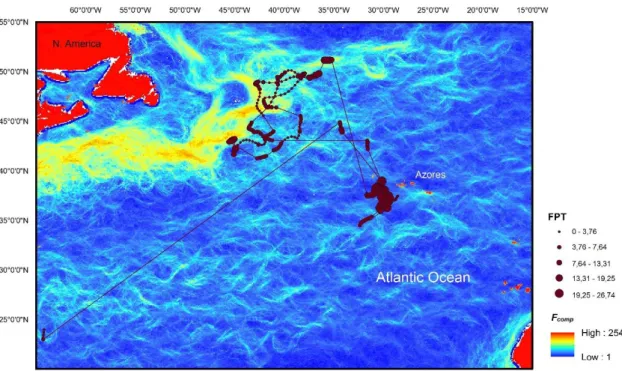
Fig. 6 – Geographical locations with FPT and correspondent Fcomp of shark A12 (9 December 2009 to 23 June 2011). Shark M2 moved northwest from the tagging location to the Gulf Stream in the early autumn until the end of the tracking period (Figure 7).

(35)

33

Relation between search effort and thermal fronts

Finally, for a better understand of the influence that thermal fronts have in the foraging behaviour I performed a GAMM for each of the studied species. GAMM results are summarized in Tables 3 and 4.

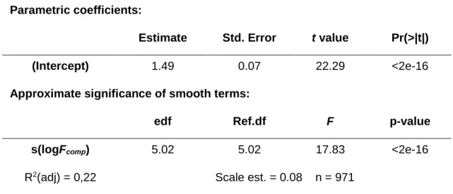
Table 3 – Summary of model results for blue sharks. Estimated parameters from the final generalized additive mixed model and numerical output for the smoothing function. edf: estimated degrees of freedom; Scale est: estimate scale parameter; R2_{: explanation for deviance; Scale est: variance of Residuals.}

Parametric coefficients:

Estimate Std. Error t value Pr(>|t|)

(Intercept) 1.49 0.07 22.29 <2e-16

Approximate significance of smooth terms:

edf Ref.df F p-value

s(logFcomp) 5.02 5.02 17.83 <2e-16

R2_{(adj) = 0,22} _{Scale est. = 0.08 n = 971}

Table 4 – Summary of model results for mako sharks. Estimated parameters from the final generalized additive mixed model and numerical output for the smoothing function. edf: estimated degrees of freedom; Scale est: estimate scale parameter; R2_{: explanation for deviance; Scale est: variance of Residuals.}

Parametric coefficients:

Estimate Std. Error t value Pr(>|t|) (Intercept) 1.70 0.09 19.12 <2e-16

Approximate significance of smooth terms:

edf Ref.df F p-value s(logFcomp) 2.86 2.86 2.06 0.11

R2_{(adj) = -0.01} _{Scale est. = 0.10 n = 265}

According to the GAMM results for blue sharks, higher frontal intensity (Fcomp) values lead to an increase in the intensity of ARS (foraging) behaviour. The R2 _{value for the}

(36)

34 model was 0.22, indicating that about 22% of the variation in logFPT can be explained by the logFcomp. The variance of the residuals is 0.08. The smoother s(logFcomp) was found to be statistically significant at the 5% level (F=17.83, p<2e−16) and thus contributed to model sharks' logFPT (Figure 8). The optimal number of degrees of freedom for the smoother was 5.02, confirming the non-linear relationship between FPT and Fcomp. There was a clear effect of frontal intensity on ARS (foraging) behaviour (Figure 8). The smoother starts with the minimum value of ~0.50, kept stable and showed a sharp increase at ~1.60 until it reaches a peak at ~2.25.

Fig. 8 – Modelling the relation between Fcomp and FPT with a Generalized Addictive Mixed Model (GAMM) for blue sharks. Fcomp had a smoothing term significantly different from zero (p<0.001) and thus contributed to model sharks' FPT. An initial

stable relation between FPT and Fcomp was observed, followed by a sharp increase in FPT with the increase of Fcomp. Dashed lines represent 95% confidence intervals above and below the solid line representing the logFPT. The little vertical lines along the x-axis indicate the FPT values of individual sharks and the y-axis the contribution of the smoother to the fitted values.

Contrary to the GAMM results obtained for blue sharks, no significant relationship was found between thermal fronts and foraging behaviour for mako sharks. The explained deviance R2 _{obtained was -0.01 which indicates that the chosen model does not follow} the trend of the data. The variance of the residuals was 0.10. The smoothing term s(logFcomp) was not a statistically significant variable, with an F value of 2.06 and p-value

(37)

35 of 0.11 (p>0.05) and an optimal number of degrees of freedom of 2.86, indicating a weak non-linear relationship between variables.

In the case of mako sharks, the smoother is centered around 0 starting a smooth decrease until a minimum of ~1.00 and increasing until it reaches a peak in ~1.75 and starts decreasing for the higher logFcomp values.

The GAMM analysis showed that, overall, tagged sharks preferred frontal boundary habitats with high SST gradients known to be highly productive.

Fig. 9 - Modelling the relation between Fcomp and FPT with a Generalized Addictive Mixed Model (GAMM) for mako sharks.

GAMM revealed no significant differences in the smoothing term (p>0.001). An initial decrease in FPT is observed, starting to increase around 1.0 with the increasing Fcomp until it reaches a pick and start a smooth decrease. Dashed lines represent

95% confidence intervals above and below the solid line representing the logFPT. The little vertical lines along the x-axis indicate the FPT values of individual sharks and the y-axis the contribution of the smoother to the fitted values.

(38)

36

Discussion

In this study, I used a large number of tracked sharks from two species ranging from 2006 to 2015, tagged with satellite tags in essentially three different areas of the north Atlantic Ocean. Individual sharks displayed relatively variable movement patterns across the various areas over timescales of days-weeks-months (Table 1), with one blue shark moving into the southern hemisphere (Figure 1; A14). Satellite tags provided data on the movements and space-use at different spatial scales and over longer time-periods, however, continuous advances in tracking technology brought more accurate tracking data that can be used in future investigations about habitat preference of marine vertebrates with more accurate data at finer scales, such as fast-acquisition GPS systems (Sims et al., 2010).

Spatial distribution

With the FPT analysis, quantification of search effort allowed the understanding of where blue and mako sharks spent more time along their pathways. The combination of FPT analysis with composite front mapping (Miller, 2009) provided a new insight into the influence of oceanic fronts in habitat selection of pelagic sharks in this study. By the observation of combined FPT data with composite front maps, there seemed to be higher FPT values in high frontal intensity areas such as the Gulf Stream and the Azores archipelago. As previously stated, higher shark densities were identified at all the locations where sharks from our study aggregated (Tittensor et al., 2010; Campana et

al., 2011).

In general, blue and mako sharks had more northward movements during spring and summer and tended to spend the cold seasons in the mid-Atlantic or in more southern regions. It is also evident a site-fidelity foraging behaviour, especially in blue sharks tagged in the Azores, returning to this area during the winter. This behaviour was also identified in other shark species (Meyer et al., 2010; Barnett et al., 2011), as also in marine predators, such as seabirds (Patrick et al., 2014) and mammals (Foote et al., 2010; Irvine et al. 2014), and may be indicative of the knowledge about prey spatial and temporal distribution acquired from previous foraging experiences (Weimerskirch, 2007; Bost et al., 2009; Wakefield et al., 2015).

(39)

37

Data analysis and results

Because of the spatial and temporal auto-correlation presented in our data I opted to perform a mixed GAM analysis for modulation. It is of great importance for the model to assume that observations from different sharks are independent, likewise for tagging locations of the same shark, because without taking the inherent individual-level variability into account, tracks with more locations could bias the results. Additionally, the GAMM analysis includes a random-effect term (Pankratz, de Andrade & Therneau, 2005) which can deal with different behavioural data among individuals.

My analysis determined a high relation between the FPT and thermal fronts in blue sharks. Although several tracks were relatively short (few days), results are indicative of the association between blue sharks with these high-density prey hotspots. Previous investigations revealed associations between marine predators with coastal and oceanic fronts. For example, Scheffer et al. (2010) investigated the foraging strategy of king penguins (Aptenodytes patagonicus) in relation to both the time of the day and variation in SST in the Polar Front Zone (PFZ). They also explored how king penguins encounter predictable oceanographic mesoscale features in the PFZ to the north of South Georgia, and, consequently, how they adjust their dive and foraging behaviours. King penguins were tracked with SPOT4 and Mk 7 WildLife Computers Time Depth Recorder (TDR), between December 2005 and January 2006, at the Hound Bay colony in the north-east of South Georgia. SST data were obtained in order to investigate correlations between foraging behaviour and oceanographic conditions. The FPT analysis was calculated to determine changes in search effort of the tracked individuals. King penguins appeared to target predictable mesoscale oceanographic features in the PFZ, as the warm-core eddy and strong temperature gradients at oceanic fronts in this area. When reaching warmer waters, two different trip types could be distinguished: the direct trips, characterized by straight pathways to one foraging area, and circular trips, where birds foraged along strong thermal gradients. Giving this, different ARS patterns were identified for the two trip types. In the direct trip type, ARS was clearly concentrated in specific areas, while for the circular trip type the ARS was displayed over the whole duration of the trip. ARS patterns are correlated with the two trip types, but the direct trips seem to represent a favorable foraging strategy. There was a clear relation between the diving behaviour with water temperature and time of day, highlighting the probable influence of prey distributions in the adjustment of foraging effort and travel patterns.

(40)

38 In contrast, model results from mako sharks revealed no significant relation between FPT and thermal fronts. We need to take into consideration that our data from mako sharks are very small compared to that for blue sharks. I am modelling data from 44 individual blue sharks against only 4 individual mako sharks. Additionally, the tracking data from these 4 individuals is also short, ranging from 23 to 58 days, most probably representing a small portion of the track. The same problem was found in the study carried out in north-east Atlantic (Miller et al, 2015) where tracking data from only seven basking sharks (Cetorhinus maximus) were associated with seasonally persistent and contemporaneous fronts. Results indicate sharks’ preference for productive regions, but obviously, these results could not be extrapolated to the population level, as it happens in the case of mako sharks from this study.

Likewise, the FPT radius had different values among species. While for blue sharks the FPT radius ranged between 25.00 and 824.70 km, for mako sharks it ranged between 58.00 and 268.55 km, which probably explains the absence of results. FPT analysis is very sensitive to telemetry error (Pinaud, 2008) and when applied at very patchy habitat conditions, it can lead to an erroneous classification of the ARS behaviour actually displayed by animals. Although I chose a common spatial scale for the studied individuals, large-scale activities may mask smaller scale behaviours (Fauchald & Tveraa 2003). Better results would be obtained if FPT radius were chosen for a finer-scale, especially in the case of sharks with short tracking data. Tracking data should be long enough so that the analysis can distinguish between extensive and sinuous movements, so probably the analysis should be re-run to identify ARS behaviour at smaller scales within the large areas of the radius with the highest variance.

In the statistic values from the GAMM, blue sharks had an R2_{value of only 0.22.} Nevertheless, this low R2_{value was expected. When for example any field attempts to} predict human behaviour, the R2_{values are typically lower than 50%, because humans} are harder to predict than their physical processes (Frost, 2013). However, the F-test indicates a statistically significant relationship between variables, which means that changes in logFPT are associated with changes in logFcomp and thus, I can still draw important conclusions. In the case of mako sharks, the R2_{is a negative value of -0.01. It} is possible to have a negative R2_{value whenever the best-fit model fits the data worse} than a horizontal line.

The explanatory variable Fcomp used in GAMM covers the frontal activity registered for the individual tracking days, giving the mean frontal activity for each of the sharks.

(41)

39 However, the GAMM would give more accurate results about the relation studied here when modulating monthly, weekly and daily composite front maps (Fcomp). For example, in the case of shark M2 there is an unquestionable relation between foraging behaviour and frontal activity and probably the GAMM results for this species would give a significant relation when running with finer-scale data.

Future work

Although the interaction between oceanography and marine predators have been predominantly studied with two-dimensional data from telemetry (Wakefield et al., 2009) it would be of great importance to analyze vertical data, especially because blue and mako sharks are deep diving predators (Carey & Scharold, 1990; Holts & Bedford, 1993) and their behaviour may be coupled to the fine-scale horizontal and vertical distributions of their prey (Elliott et al., 2008; Queiroz et al., 2012, 2017; Boyd et al., 2015; Goldbogen

et al., 2015). When studying environmental processes, composite front mapping can only

detect surface frontal activity giving a two-dimensional view of a complex three-dimensional environment. Moreover, our study does not include the effects of mixed-layer depth, thermocline, chl-a fronts, oxygen concentration and other oceanographic factors found to have an influence on the habitat selection by predators (McConnell et

al., 1992; Cotté et al., 2007; Nordstrom et al., 2013; Scales et al., 2014a).

In the study of Queiroz et al. (2017), high-resolution dive depth profiles were analyzed for blue and basking sharks, tagged with PSAT tags in the north Atlantic, to examine movement patterns in relation to environmental heterogeneity. U- and V-shaped dives were the most commonly performed by both species, representing ∼70% of the total number of dives. They found that mean depth and mean depth range decreased with increasing levels of primary productivity (chl-a), whereas ascent velocities displayed a positive correlation. By combining dive profiles with horizontal movements and oceanographic gradients, blue sharks were found to forage closer to the surface in productive areas of the north Atlantic, where surface longliners also concentrate their activities (Queiroz et al., 2012).

In future work, horizontal interactions with frontal activity could be compared with vertical data from the same individual, incorporating other oceanographic features in these models. New improvements on tracking devices allowed collection of three-dimensional information about the behaviour of diving animals, such as altimetry of Global Positioning Systems (GPS), acoustic systems, geomagnetic intensity, dead reckoning or digital tags