Shallow water tomography with a sparse array
during the INTIMATE’98 sea trial
P. Felisberto, S. Jesus
Y. Stephan, X. Demoulin
SiPLAB, University of Algarve EPSHOM/CMO
Campus de Gambelas Rue du Chatellier
Faro,Portugal Brest,France
{pfelis,sjesus}@ualg.pt {stephan,demoulin}@shom.fr
Abstract — Invert acoustic data using sparse arrays - at the limit with a single hydrophone - is a challenging task. The final goal is to obtain a rapid environmental assessment with systems both easier to deploy and less expensive than full vertical arrays. In this paper, it is shown that using a known broadband source signal and an array with few hy-drophones, ocean acoustic tomography can be performed, even in a complex internal waves induced highly variable
ocean. The inversion approach presented herein is based
on an arrival matching processor and a genetic algorithm search procedure. Due to the poor accuracy on the a pri-ori knowledge of the source range, source depth and water depth, the inversion procedure was split in two stages: in the first stage the geometric parameters where estimated and in the second stage sound speed estimates where ob-tained. This procedure was applied to field data, acquired during the INTIMATE’98 sea trial, in a shallow water area off the coast of France in the Gulf of Biscay. That area is expected to have a relatively high internal wave
activ-ity, specially during the summer. A 4 sec long - 700 Hz
bandwidth linear frequency modulated signal was transmit-ted from a ship suspended sound source and received on a 4 element vertical array at a range of approximately 10.5 km, over a relatively range-independent area. The results from the inversion of the acoustic data are in line with those obtained by concurrent non acoustic data like GPS source range, measured source depth, XBT casts and temperature sensors.
I. Introduction
In nowadays, rapid environmental assessment by acous-tic means is a subject of intense research [1]. In this con-text it is important to use light receiving acoustic systems that are easier to deploy and less expensive then full length vertical arrays. This paper describes the results of acous-tic inversions achieved with a sparce 4 hydrophone veracous-tical array during the INTIMATE’98 experiment [2], that took place in a shallow water area off the coast of France in the Gulf of Biscay. This work, experimentally demonstrates, that using a known broadband source, in our case with a bandwidth of 700Hz, acoustic tomography is possible with a relatively simple receiver in an internal waves induced highly variable environment.
The results presented are for different stages of acoustic inversion: source range and source depth, water depth and sound speed profile. In this work the inversion of acoustic data is stated as an optimization process, where brute force search and genetic agorithms were used to found a modeled signal that minimizes the misfit with a measured signal.
II. The experimental setup
The INTIMATE’98 experiment was dedicated to inter-nal wave tomography in 4 areas of the Gulf of Biscay [3][4]. The observations were carried out in the period of 25 June until 30 July 1998. Figure 1 shows the position of the dif-ferent instruments. This work will focus on acoustic data acquired on moored arrays at positions G1 and G2, ctd data acquired on position G11 and temperature sensors data acquired on position M3. The sound source is sus-pended from a ship at position G0. The bathymetry is range independent along G0-G1 line, and slightly range dependent along G0-G2 line with a upslope of 10m. Ac-cording to independent direct measurements, the bottom characteristics are approximately homogeneous along both lines. Table I summarizes the mean values of the baseline environment [5].
Each array has 8 hydrophones at depths ranging from 34m to 104m at 10m spacing. The hydrophone at 54m in G1 and the hydrophones at 94m and 104m at G2 were not working.
TABLE I
Baseline environment parameters
G0-G1 G0-G2
source range 10.450m 9.450m
source depth 74m 74m
water depth 146m 146m-136m
bottom density 1.95 1.95
bottom absorb. coef. 0.7dB/λ 0.7dB/λ
bottom compres. velo. 1750m/s 1750m/s
The signal emitted is a 300-1000Hz linear frequency mod-ulated (lfm) pulse in the sequence: 2s duration lfm, 2s idle, 4s duration lfm, 4s idle.
Figure 2 presents the mean sound speed profile as mea-sured from ctd data captured during a period of 20 hours at G11 (a), and the first 2 empirical orthogonal functions(eof) derived from this data set (b). One can observe a well de-fined thermocline between 15m and 25m. The first 2 eofs were used since they account for more then 90 percent of the energy.
−5.3 −5.25 −5.2 −5.15 −5.1 −5.05 47.16 47.17 47.18 47.19 47.2 47.21 47.22 47.23 47.24 G0 G1 G2 G11 M3 (source) (array) (array) (ctd) (temp. sens.) Latitude ( ° ) Longitude (°)
Fig. 1. INTIMATE’98 instrument localization: G0 source; G1,G2 vertical arrays; G11 ctd; M3 temperature sensor line.
0 50 100 150 1495 1500 1505 1510 1515 a) water depth(m) sound speed (m/s) 0 50 100 150 −0.4 −0.2 0 0.2 0.4 b) eof1 eof2
Fig. 2. a) Mean sound speed profile. b) First 2 empirical orthogonal functions from ctd data
III. The arrival pattern matched processor The processor used for acoustic inversion is a slightly adapted processor from that proposed by Porter et al in [6]. The received data is pulse compressed, that is the received waveform is correlated with a replica of the transmitted sig-nal. After pulse compression, the envelopes are computed and averaged - 10 in our case - to stabilize the estimates. The obtained signal is generally called as arrival pattern, since it emphasizes the echo structure of the transmission channel. To avoid unknown signal amplitude fluctuations the averaged arrival patterns have normalized energy. The obtained arrival pattern is noted as a(t). In order to bal-ance weak and strong echoes in the arrival pattern the log is computed:
r(t) = 20∗ log(a(t)) + k, (1)
where k is a constant set to 30dB that shifts log-arrival patterns to positive values. Using an ocean-acoustic model and the apriori knowledge of the emitted source signal, the modeled arrival pattern m(t, φ) is computed with a proce-dure equivalent to the one described above, where φ repre-sents the model parameters. The measure of misfit between
measured arrival patterns and simulated ones is done by correlation:
y(t, φ) = Z
r(τ )m(τ− t, φ)dτ, (2)
where the fit is
f (φ) = max
t |y(t, φ)|. (3)
Next, the inversion is formulated as an optimization pro-cedure, looking for the maximum of f (φ). Brute force and genetic algorithms based search will be used. Note that this processor operates on a single hydrophone, while an extension to N hydrophones uses the geometric average,
f (φ) = N v u u t N Y i=1 fi(φ), (4)
where fi(φ) is the fit associated to hydrophone i, i =
1, . . . , N .
IV. Inverting for source range and source depth The first step in acoustic data inversion addresses the estimates of source range and source depth. The source range was sampled from 6km to 13km with a sampling interval of 50m, the source depth was sampled at depths 55, 60, 65, 70, 72, 74, 78, 80, 85, 90 and 95 meters. The sound speed profile used to generate simulated arrival patterns was extracted from one of the ctd casts acquired during the period of observation. The bottom characteristics and water depth values were those of table I. The optimization procedure was a brute force search. The model CSNAP [7] was used to generate arrival patterns.
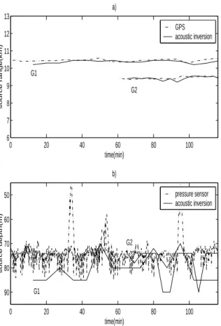
Figure 3 compares the obtained estimates, source range fig. 3a and source depth fig. 3b, with those obtained by non acoustic means -GPS and pressure sensor respectively. Since the acquisition start time is different for each array, there is about two hours observation period for G0-G1 the range independent track and one hour for the G0-G2 range dependent track. Labels G1 and G2 point out the start of the respective period. The inversion results were achieved using hydrophones that are well bellow the thermocline (at 74m, 84m, 94m and 104m for G1 and 74m and 84m for G2). One can remark that acoustic inversions results agree with the GPS data both for the range independent track and for the range dependent track, even for source depth, which pressure sensor denotes important instantaneous variability.
V. Multistage inversion of sound speed profile Since our goal is to invert the sound speed profile, the next step was to decrease the search space for source range and source depth, using the information available from nav-igation system and introduce new parameters in the search: sound speed profile represented by two eofs and the water depth that is generally a relevant parameter. The opti-mization is from now on implemented by genetic algorithm
0 20 40 60 80 100 6 7 8 9 10 11 12 13 time(min) source range(km) a) GPS acoustic inversion 0 20 40 60 80 100 50 60 70 80 90 source depth(m) time(min) b) pressure sensor acoustic inversion G1 G2 G1 G2
Fig. 3. Source range and source depth estimates for range inde-pendent track (G1) and range deinde-pendent (G2) during a period of 2 hours: a) source range, b) source depth. Results from acoustic inver-sions are represented by solid line; results from non acoustic means (GPS, pressure sensor) by dash dot lines.
(GA) search, since search space grows exponentially with the number of parameters. The fit function used in GA is computed by expression (4) from acoustic data of hy-drophones at 74m, 84m, 94m, 104m (G0-G1) track. The PROSIM model [8] is used to compute the arrival patterns, since this model is more efficient for broadband calcula-tions than CSNAP and computation time is of concern here. Only inversions from the range independent track are discussed next (G0-G1 track). The final results are ob-tained from a multistage procedure, where from one stage to the next we use the last stage estimates to reduce the search space.
A. Water depth estimates
The water depth fluctuation around a mean value highly depends on barotropic tide. In our case, following a tidal model [9], the peak to peak tide amplitude is about 3m. In this stage the main goal is to estimate water depth as function of time and verify the agreement of those estimates with the tidal model. The search space and the parameter discretization is summarized in table II.
The stars in figure 4 represent the inversion estimates. The continuous curve superimposed in this figure is ob-tained from the tidal model offset by the mean water depth. It can be remarked that the evolution of the acoustic
TABLE II
Parameters range and discretization step for water depth estimation
Parameter min. value max. value step size
source range 10.200m 10.500m 2.36m
source depth 70m 90m 0.32m
coef. first eof -20 20 0.63
coef second eof -10 10 0.65
water depth 142m 150m 0.13m 189.35 189.4 189.45 189.5 189.55 189.6 189.65 189.7 189.75 189.8 142 143 144 145 146 147 148 149 150 julian time(day) water depth (m)
Fig. 4. Water depth estimates (stars) and true water depth corrected with tide estimates (solid line)
estimates of water depth is in agreement with the tidal model. Also the source range and source depth inversions (not presented here) are in agreement with navigation data. B. Sound speed estimates
In this stage we restrict even more the search space for the parameters: source depth, source range, and water depth. Only the search space for eof coefficients are not restricted from the previous stage. Table III summarizes the new search intervals and their discretization for the var-ious parameters. Figure 5 illustrates the inversion results obtained for the eof coefficients during G0-G1 track. For each arrival pattern the inversion was done by several in-dependent runs of the GA to avoid the dependence on the initialization. In the figure, the best individual of each in-dependent run for a given arrival pattern is represented by a star, a circle, a square a pentagram or a hexagram. One can see that for the great part of cases the best values found for the various coefficients are in the neighbourhood of the best of the bests, which denotes the convergence of the ap-plied method. The best of the best values are joined by solid curves. The dash dot curves connect coefficients that are projections of ctd casts to the first eof (α1) and second
eof (α2). The plus symbol defines the time where ctd casts
were performed. The comparison between acoustic inver-sions and measured values should be done with caution: ctd data are point measurements, but acoustic inversion accounts for integral data, i.e. for the ”mean” sound speed
TABLE III
Search interval definitions for eof coefficients search
Parameter center half interval l step
value length size
source range GPS mean value (2 mins) 75m 2.38m
source depth depth sensor mean value (2 mins) 5m 0.32m
first eof coef. 0 20 0.32
second eof coef. 0 10 0.32
water depth estimated curve (fig. 4) 1m 0.13m
189.65 189.7 189.75 189.8 −20 −10 0 10 20 30 − − − − − − − − − − − − − − − − − − − − − − − − − − − − − − − − − − − − − − − − − − − − − − − − − − − − − − − − − − − − − − − − − − − − − − − − − − − − − − − − − − − − − − − − − − − − − − − − − − − − − − − − − − − − − − − − − − − − − − − − − − − − − − − − − − − − − − − − − − − − − − − − − − − − − − − − − − − − − − − − − − − − − − − − − − − − − − − − − − − − − − − − − − − − − − − − − − − − − − − − − − − − − − − − − − julian time(days) α1 189.65 189.7 189.75 189.8 −10 −5 0 5 10 − − − − − − − − − − − − − − − − − − − − − − − − − − − − − − − − − − − − − − − − − − − − − − − − − − − − − − − − − − − − − − − − − − − − − − − − − − − − − − − − − − − − − − − − − − − − − − − − − − − − − − − − − − − − − − − − − − − − − − − − − − − − − − − − − − − − − − − − − − − − − − − − − − − − − − − − − − − − − − − − − − − − − − − − − − − − − − − − − − − − − − − − − − − − − − − − − − − − − − − − − − − − − − − − − − julian time(days) α2
Fig. 5. First (α1) and second (α2) eof coefficient inversion results for the G0-G1 track:star, circle, square, pentagram, hexagram - best individual for a search algorithm run; solid curves - joins the best of the bests fits; plus symbol - points of ctd casts; dash dot curves - join points of ctd casts.
profile between sound source and array. Also, the ctd casts are acquired every half an hour, which is not sufficient for properly sampling the sound speed perturbations due to internal waves observed in the experiment area [5]. The in-ternal wave phenomenon could be the justification for the variability observed on acoustic inversions.
Figure 6 presents a more significative comparison be-tween acoustic inversions and non acoustic measures of sound speed. That figure shows the time evolution of a
15.5◦C isothermic (solid line), and the corresponding 1506
ms−1 isovelocity line (dash dot). Those values are related
by an approximation of the Mackenzie formulae [10] to the linear and quadratic dependence of sound speed on temper-ature. The isothermic line is derived from data acquired by temperature sensors M3 (see figure 1) which is in a middle
189.65 189.7 189.75 189.8 15 20 25 30 35 40 45 50
julian time (day)
depth(m)
isothermic line 15.5°C (temp. sensors) isovelocity line 1506ms−1(acoust. inver.)
Fig. 6. Comparison between acoustic estimates and temperature sensors measurements(M3): solid line is a 15.5◦C isothermic line from temperature sensors, dash dot line is a 1506ms−1isovelocity line from acoustic inversions.
position between sound source and array. The sampling
frequency is 1 sample per second. The 15.5◦C was chosen
because it represents a middle value of the thermocline.
The corresponding sound speed 1506 ms−1is derived from
estimated eof coefficients, by acoustic inversions.
Analyzing the figure, one can say that the results from acoustic inversions are in line with non acoustic measure-ments: during the period of observation only one inver-sion is clearly out of the general trend(around julian date 189.75), the shape of the curves is similar and only a offset can be identified in the second half of acoustic inversions.
VI. Conclusion
The INTIMATE98 data set processed in this paper emphasizes that with a reduced number of hydrophones, one can derive information about source-receiver geome-try, barotropic tide and baroclinic tide. It was shown that with a simple array of 4 hydrophones sound speed pertur-bations can be tracked in challenging environments where internal waves activity is important. The achieved results are remarkable since this is an environment with impor-tant sound speed fluctuations, the geometrical parameters are not well known a priori, source-array synchronization is not available and the array has a small number of hy-drophones. This work is intended to be a contribution to
the feasibility study of a light acoustic monitoring system for rapid environmental assessment.
References
[1] P. Elisseeff, H. Schmidt, M. Johnson, D. Herold, N. R. Chap-man, and M. M. McDonald. Acoustic tomography of a coastal front in haro strait, british columbia. Journal Acoust. Soc. Am., 106(1):169–184, July 1999.
[2] Y. Stephan, T. Folegot, J. Lecullier, X. Demoulin, and J. Small. The intimate98 experiment. In Proc. of the Fifth European Con-ference on Underwater Acoustics, volume 2, pages 1329–1334, 2000.
[3] Y. Stephan, T. Folegot, J. Lecullier, X. Demoulin, and J. Small. Internal tides investigation by means of acoustic tomography experiment at the shelf break at the bay of biscsy in 1998. In Procceding of the International Acoustical Oceanography Con-ference, Southamptom, April 2001.
[4] Y. Stephan, T. Folegot, J. Lecullier, X. Demoulin, and J. Small. Intimate98 data report: Hydrology. Technical Report 01, EPSHOM/CMO/OCA/NP, 1999.
[5] T. Folegot Small. Intimate98 etude du probleme direct. Techni-cal Report 01, Atlantide, 1999.
[6] M-B. Porter, S.M. Jesus, Y. St´ephan, E. Coelho, and X. D´emoulin. Single-phone source tracking in a variable en-vironment. In Proceedings of the Fourth European Conference on Underwater Acoustics, Rome,Italy, 1998.
[7] C.M. Ferla, M.B. Porter, and F. B. Jensen. C-snap: Coupled saclantcen normal mode propagation loss model. Technical Re-port SM-274, SACLANTCEN, La Spezia, Italy, 1993.
[8] F. Bini-Verona, P. L. Nielsen, and F. B. Jensen. Prosim broad-band normal-mode model - a users guide. Technical Report SM-358, SACLANTCEN, La Spezia, Italy, ?
[9] R.D. Ray, B.V. Sanchez, and D.E. Cartwright. Some ex-tensions to the response method of tidal analysis applied to topex/poseidon altimetry. EOS Trans., 75, 1994.
[10] K. V. Mackenzie. Nine-term equation for sound speed in the oceans. Journal Acoust. Soc. Am., 70:807–812, 1981.