Analysis and characterisation of masonry walls

(1)

F

ACULDADE DE

E

NGENHARIA DA

U

NIVERSIDADE DO

P

ORTO

Analysis and Characterisation of

Masonry Walls

Pedro Trigueiros de Sousa Pereira

Mestrado Integrado de Engenharia Electrotécnica e Computadores Supervisor: Miguel Velhote Correia (PhD)

(2)

c

(3)

(4)

(5)

i

(6)

(7)

Resumo

A preservação e valorização do património construído é uma preocupação da maior actualidade. Parte significativa desse património é constituída por estruturas de alvenaria de pedra, em grande parte na forma de paredes. Preservar esses elementos requer conhece-los adequadamente quanto à sua constituição, procurando avaliar as quantidades e mapear a distribuição dos materiais consti-tuintes, nomeadamente a pedra e a argamassa eventualmente existente nas juntas de contacto entre as pedras. Esse mapeamento deverá permitir contabilizar as quantidades (em termos de área) de cada um desses componentes existentes nas faces da parede analisada. São apresentados alguns métodos de processamento e análise de imagem utilizados noutras áreas e diferentes algoritmos que abordam as características da textura das imagens.

(8)

(9)

Abstract

The preservation and valuation of the constructed patrimony is an actual concern. Significant part of this patrimony is constituted by rock masonry structures, to a large extent in the form of walls. To preserve these elements it’s required to know its constitution, to evaluate the amounts and to map the distribution of the materials constituents,namely the mortar existing in the meetings of contacts between the rocks. This mapping will have to allow to enter the amounts (in area terms) of each one of these existing components. Some methods of processing and analysis of image used in other areas and different algorithms are presented that aproach the texture features of the images.

(10)

(11)

Acknowledgments

My first thanks goes to my supervisor Professor Miguel Correia for proposing this challenging project and helping me acquire the necessary knowledge to comprehend and implement the differ-ent concepts, and for keeping me motivated throw out the developing of the work.

I would like to thank the Laboratório de Engenharia Sísmica e Estrutural (LESE), in partic-ular Enga_{. Celeste Almeida for the digital material made available for creating the database for}

developing this work.

Finally, my parents, brothers, sisters and Ana for their encouragement, support and love throughout my college years.

(12)

(13)

List of Figures

1.1 The Great Wall of China . . . 1

2.1 Pixel (0,0) spatial reference . . . 3

2.2 Different types of images . . . 5

2.3 Examples of different textures . . . 6

2.4 The original LBP operator . . . 9

2.5 Circular neighbors for different values of P and R . . . 10

3.1 Learning the Texton Dictionary . . . 12

3.2 Multiple models per texture . . . 12

3.3 Nearest Neighbour classification . . . 13

3.4 Classification without filtering . . . 14

4.1 Single texture images . . . 18

4.2 Two texture classes images . . . 18

5.1 Different classification results . . . 21

5.2 Calculating distances between textons of different dictionaries, and pair wise dis-tances . . . 22

(16)

(17)

List of Tables

2.1 Texture features . . . 9

5.1 Single texture classification results . . . 20

B.1 Confusion Matrix Image 1 . . . 27

B.2 Confusion Matrix Image 2 . . . 27

(18)

(19)

Chapter 1

Introduction

1.1 Motivation

Some of the world’s most significance architectural structures have been built with masonry, the Egyptian Pyramids, the Colosseum in Rome, India’s Taj Mahal, the Great Wall of China. The level of complexity involved in masonry work varies from laying a simple masonry wall to installing an ornate exterior or high-rise building. Along History, architects and constructors have used this technique for its beauty, versatility and durability. Masonry buildings are resistant to fire, earthquakes, sound as well as the deterioration of time [1].

Figure 1.1: The Great Wall of China

Buildings are an historical and cultural inheritance. Despite its huge durability, the construc-tions with masonry are not eternal. From the will to keep and restore historical buildings was

(20)

2 Introduction

born the necessity to study the structure and composition of these constructions. Defining the vulnerability of the buildings and evaluating the different techniques for repairing became of great importance.

Binda and Cardani [2] defined a method for analysis of the vulnerability of a building through an analysis of the History, materials, morphology of a section of the wall, the damage mechanism and the effectiveness of the re-qualification techniques. A sorting of the different types of wall is accomplished through graduated photograph analysis, taken parallel to the surface. Over the image all stones, mortar and holes are identified. The occupied surface for the different materials is measured, allowing to evaluate the rock and mortar percentages as the dimension and distribution of defective. With the knowledge of the morphology it’s possible to use models of the geometry and mechanical behavior of the wall.

When done manually the representation of each material in the wall is a systematic and time consuming process. The use of digital photograph allows this work to be accomplished automat-ically using digital image analysis and processing techniques. Segmentation and classification techniques using texture analysis can be used to extract the morphology of masonry walls [3]. The Laboratório de Engenharia Sísmica e Estrutural (LESE) presented the challenge to develop an algorithm able of distinguish the different elements on a masonry walls an integrate it with the laboratory applications using LabView.

1.2 Goal of the work

Literature is scarce in aiming at the goal of distinguishing mortar from stone using texture analysis. We can find different works concerning the classification of different texture material [4]. Capua

et al.[5] presented a methodology to analyse masonry structures using digital photography. The authors employ image processing techniques to a digital image to obtain a finite element mesh.

The work presented in this dissertation intends to find a methodology able to identify different types of mortar and stone in different masonry structures. To study texture analysis by applying methods to a database of collected images of masonry walls. Implement known methods and apply to classification, labeling different elements present in masonry images and integrate the developed methods with LabView.

1.3 Thesis Organization

The thesis is organized in the following manner. In Chapter 2, several digital image definitions are presented and described, and contain a literature review. Chapter 3, contains a description of the classifier implemented in the methodology. In Chapter 4 the database used is presented. Chapter 5 explains the used methodology and experiment design. Chapter 6 presents a discussion of the results and future work and extensions.

(21)

Chapter 2

Texture Image Analysis

2.1 Digital Images

A digital image is a two dimension matrix representing the light intensities values distributed in space. It is a bidimensional function of light intensity,

f (x,y)

where f is the luminosity of the point (x,y), x and y represent the space co-ordinates of a image element, the pixel.

By convention the point (0,0) is the left upper corner of the image. The value of x grows from left to right while y from up to down.

Figure 2.1: Pixel (0,0) spatial reference

Digital images are obtained by a sensor (camera, scanner) that converts a image into a discrete number of pixels. To each pixel is attributed a spacial position and grayscale or color value. A digital image has three fundamental properties[6]:

1. Resolution: it is determined by the number of rows and columns of pixels. An image with

(22)

4 Texture Image Analysis

2. Definition: indicates the number of different pixel values. The bit depth is the number of bits used to encode the value of the pixel. For a given bit depth of n, the image has an image definition of 2n_{, the same is to say that a pixel can have 2}n_{different values.}

3. Number of Planes: corresponds to the number of arrays of pixels that compose the image. A grayscale image is composed by one plane. A color image is the combination of three arrays of pixels corresponding to the red, green, and blue components in an RGB image. HSL images are defined by their hue, saturation, and luminance values.

2.1.1 Grayscale Images

In a grayscale image each pixel is encoded using one of the following single numbers:

• An 8-bit unsigned integer representing grayscale values between 0 and 255. • A 16-bit unsigned integer representing grayscale values between 0 and 65535. • A 16-bit signed integer representing grayscale values between -32768 and 32767.

• A single-precision floating point number, encoded using four bytes, representing grayscale

values ranging from−∞ and +∞.

2.1.2 Color Images

A color image is encoded in memory as either a RGB or a HSL image. Color image pixels are a composite of four values. RGb images store color information using 8 bits each for the red, green, and blue planes. In HSL images the color information is stored using 8 bits each for hue, saturation, and luminance. RGB U64 images store color information using 16 bits for each plane. In the RGB and HSL color models, an additional 8-bit value is used for overlays. this representation is known as 4× 8-bit or 32 bit encoding.

2.1.3 Complex Images

A complex image contains the frequency information of a grayscale image. A complex image can be the result of a Fast Fourier transform (FFT) applied to a grayscale image. Each pixel in a complex image is encoded as two single-precision floating-point values, which represent the real and imaginary components of the complex pixel. Through the performance of different frequency domain operations on the image the real part, imaginary part, magnitude, and phase can be extracted.

2.2 Image Textures

The human vision system (HVS) is able to distinguish different materials at a glance, mainly thanks to different textures. Objects, or object surfaces, can be segmented from each other ac-cording to the degree of uniformity of the light reflected from them. This is only possible if a

(23)

2.2 Image Textures 5

(a) RGB color space (b) Grayscale Image

(c) Complex Image

Figure 2.2: Different types of images

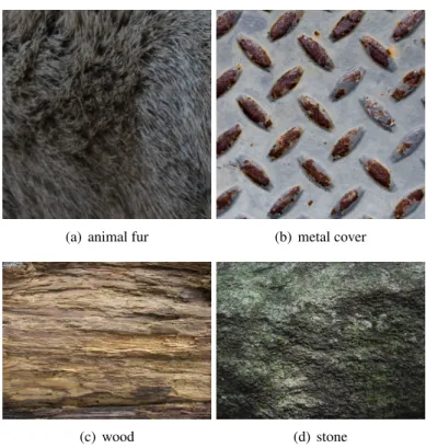
homogenous surface with uniform reflectivity is subject to uniform illumination [7]. We recognise texture when we see it but it is very difficult to define. Different texture definitions by visions researchers are shown:

"We may regard texture as what constitutes a macroscopic region. Its structures is simply attributed to the repetitive patterns in which elements or primitives are ar-ranged according to a placement rule." [8]

"A region in an image has a constant texture if a set of local statistics or other local properties of the picture are constant, slowly varying, or approximately periodic." [9] "The image texture we consider is non figurative and cellular... An image texture is described by the number and types of its (tonal) primitives and the spatial organisation or layout of its (tonal) primitives... A fundamental characteristic of texture: it cannot be analysed without a frame of reference of tonal primitive being stated or implied. For any smooth gray-tone surface, there exists a scale such that when the surface is examined, it has no texture. Then as resolution increases, it takes on a fine texture and

(24)

"Texture is defined for our purposes as an attribute of a field having no components that appear enumerable. The phase relations between the components are thus not ap-parent. Nor should the field contain an obvious gradient. The intent of this definition is to direct attention of the observer to the goal properties of the display - i.e., its over-all "coarseness", "bumpiness", or "fineness". Physicover-ally, none numerable components will include many deterministic (and even periodic) textures." [11]

(a) animal fur (b) metal cover

(c) wood (d) stone

Figure 2.3: Examples of different textures

2.3 Common Applications

There are a variety of applications domains where texture analysis methods have been utilized. Automated inspection, medical image processing, document processing, etc. The texture role varies depending upon the application. Two different domains are presented where texture analysis take an important role in achieving useful results in an industrial medium as well in medical applications.

2.3.1 Industrial Inspection

In modern assembly lines the production cadence is very high, while individual product inspection is a time consuming task impossible to be done by humans in a competitive rate. To solve this problem image analysis methods are utilized to inspect the product quality. Texture images were

(25)

2.4 Review of Texture Analysis Methods 7 used in the detection of defects in the domain of textile inspection. Dewaele et al. [12] used filtering methods to detect point defects and line defects in texture images. They used sparse convolution masks in which the bank of filters are adaptively selected depending upon the image to be analysed. Texture features are computed from the filtered images. A Mahalanobis distance classifier is used to classify defective areas. Chetverikov [13] defined a simple window difference operator to the texture features obtained from simple filtering operations. This allows to detect the boundaries of defects in the texture. A method using a structural approach is used by Chen and Jain [14] to detect defects using texture images. The skeletal structure from images is extracted, anomalies are detected by an analysis of the statistical features. Conners et al. [15] utilized texture analysis methods to detect defects in lumber wood automatically. Based on tonal features such as mean, variance, skewness, and kurtosis of gray levels along with texture features computed from gray level co-occurrence matrices the defect detection is performed by dividing the image the image into sub-windows and classifying each into one of the defect categories[3].

2.3.2 Medical Image Analysis

Image analysis techniques have played an important role in several medical applications. In gen-eral, the applications involve the automatic extraction of features from the image which are then used for a variety of classification tasks, such as distinguishing normal tissue from abnormal tissue. Sutton and Hall [16] propose the use of three types of texture features to distinguish normal lungs from diseased lungs. Interstitial fibrosis, affect the lungs in such a manner that texture changes are clear in the X-Ray images. Texture features are computed based on an isotropic contrast measure, a directional contrast, and a Fourier domain energy sampling. Harms et al. [17] diagnosed leukemic malignancy in samples of stained blood cells using image texture combined with color features. Texture features from "textons", regions with almost uniform color, were extracted. The number of pixels with a specific color, the mean texton radius and texton size for each color and various texton shape features. In combination with color, the texture features significantly improved the correct classification rate of blood cell types[3]. Sousa [18] used color and texture features of images obtained from endoscopy procedures to understand their importance for a computer-assisted medical diagnosis of precancerous and cancerous lesions.

2.4 Review of Texture Analysis Methods

Identifying the perceived qualities of texture in an image is an important step towards building mathematical models for texture. The intensity variations in an texture image are generally due to some underlying physical variation. One of the defining qualities of texture is the spatial distri-bution of gray values. The use of statistical features is therefore one of the methods proposed in machine vision literature. Model based texture analysis methods are based on the construction of an image model that can be used to describe texture. The model parameter capture the essential

(26)

2.4.1 Autocorrelation Features

The repetitive nature of the placement of texture elements is a property that can be used in texture analysis. The regularity as well the fineness/coarseness of a image is quantifiable by the autocor-relation function. Formally, the autocorautocor-relation function of an image I(x,y) is defined as follows:

ρ(x,y) = ∑Nu=0∑Nv=0I(u,v)I(u + x,v + y)

∑N

u=0∑Nv=0I2(u,v)

If the texture is coarse, then the autocorrelation function will drop off slowly; otherwise, it will drop off very rapidly. For regular textures, the autocorrelation function will exhibit peaks and valleys.

2.4.2 Random Field Models

Markov random fields (MRFs) are able to capture spatial information in an image. The models as-sume that the intensity at each pixel in the image depends on the intensities of only the neighboring pixels. The image is represented by an N × M matrix L, where

L = {(i, j)|1 ≤ i ≤ N,1 ≤ j ≤ M}

I(i, j) is a random variable which represents the grey level at pixel (i, j) on matrix L

Markov random field theory provides a convenient and consistent way to model context-dependent entities such as image pixels and correlated features. This is achieved by characterizing mutual influences among such entities using conditional MRF distributions. In an MRF, the sites in S are related to one another via a neighborhood system, which is defined as N = {Ni,i ∈ S},

where Ni is the set of sites neighboring i, i /∈ Ni and i ∈ Nj ⇐⇒ j ∈ Ni. A random field X said

to be an MRF on S with respect to a neighborhood system N if and only if

P(x) > 0,∀x ∈ X P(xi|x_S−{i}) = P(xi|xNi)

for more details about Mark Random Fields see [19].

2.4.3 Co-occurence Matrix

The use of grey level co-occurrence matrices (GLCM) has become one of the most well-known and widely used in extraction of texture features. Spatial grey level co-occurrence estimates properties related to second-order statistics. The G × G grey co-occurrence matrix Pd for a displacement

vectord = (dx,dy) is defined as: the entry (i, j) of Pd is the number of occurrences of the pair of

grey levels i and j which are a distanced apart.

(27)

2.4 Review of Texture Analysis Methods 9 where (r,s),(t,v) ∈ N × N,(t,v) = (r + dx,s + dy), and |.| is the cardinality of a set. The co-occurrence matrix reveals certain properties about the spatial distribution of the grey levels in the texture image. For example, if most of the entries in co-occurence matrix are concentrated along the diagonals, then the texture is coarse with respect to the displacement vectord. The Table2.1

lists some os the features that can be computed from the co-occurrence matrix [10].

Feature

Formula

Energy

∑

i

∑

j

P

d2

(i, j)

Entropy

−∑

i

∑

j

P

d

(i, j)logP

d

(i, j)

Contrast

∑

i

∑

j

(1 − j)

2

P

d

(i, j)

Homogeneity

∑

i

∑

j _{1+|i− j|}Pd(i, j)

Correlation

∑i∑j(i−µx)( j−µy)Pd(i, j)

σxσy

Table 2.1: Texture features

2.4.4 Local Binary Patterns

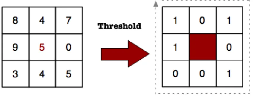
With the Local Binary Patterns (LBP) operator it is possible to describe the texture and shape of a digital (grey scale) image. The LBP of a pixel compares the grey value of that pixel to grey value of pixels in its neighborhood.

The original LBP operator was introduced by Ojala [20]. The eight neighbors of a pixel are considered, the center pixel value is used as a threshold. If a neighbor pixel has a higher (or the same) grey value than the center pixel a one is assigned to that pixel, else it gets a zero. The LBP code for the center pixel is then produced by concatenating the eight ones or zeros as a binary code.

Figure 2.4: The original LBP operator

(28)

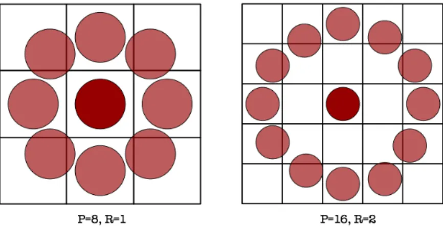
Figure 2.5: Circular neighbors for different values of P and R

the value of the center pixel. The values of all sampling points for any radius and any number of pixels is obtained by bilinear interpolation.

2.4.4.1 Uniform Local Binary Patterns

A LBP is called uniform if it contains at most two bitwise transitions from 0 to 1 or vice versa. Since the binary string is considered to be circular only one transition is not possible. For patterns with two transitions there are P(P-1) combinations possible. for uniform patterns with P sampling points and radius R the notation LBP (u2; P,R) is used.

The use of uniform LBP has two important benefits: the first is the memory used, with non-uniform patterns there are 2P _{possible combinations, with LBP (u2; P,R) there are P(P-1)+2; the}

second is that LBP (u2) detects only the important local textures, like spots, line ends, edges and corners.

(29)

Chapter 3

The Varma-Zisserman Classifier

3.1 The Varma-Zisserman Classifier

The Varma-Zisserman (VZ) classifier is divided into two stages: a learning stage and a classifi-cation stage. In the learning stage texture models are learnt from training examples by building statistical descriptions of filter responses. In the classification stage the novel images are classified by comparing their distributions to the learnt models[4].

3.1.1 The Learning Stage

In this stage a set of different training images is convolved with a MR8 filter bank. The MR8 filter bank consists of 38 filters but only 8 filters responses. The filters include a Gaussian and a Laplacian of a Gaussian filter, an edge filter at 6 orientations and 3 scales and a bar filter also at 6 orientations and the same 3 scales. The filter responses represent each image pixel in a fea-tures space of size 8. All the new pixels coordinates are aggregated and clustered. The clusters centers are calculated using the k-means algorithm [21]. The resultant cluster centers of exemplar filter responses which are called textons form the Texton Dictionary. Textons refer to fundamental micro-structures in natural images and are considered as the atoms of pre-attentive human percep-tion (Julesz, 1981).

Once the texton dictionary is calculated the texture model, of each training image, can be created and learned. Each pixel is labeled with the texton that lies closest to it in filter response space using the euclidean distance. The normalized frequency histogram of textons is the texture model. A texture class can be represented by a different number of models depending on the training images.

(30)

12 The Varma-Zisserman Classifier

Figure 3.1: Learning the Texton Dictionary

Figure 3.2: Multiple models per texture

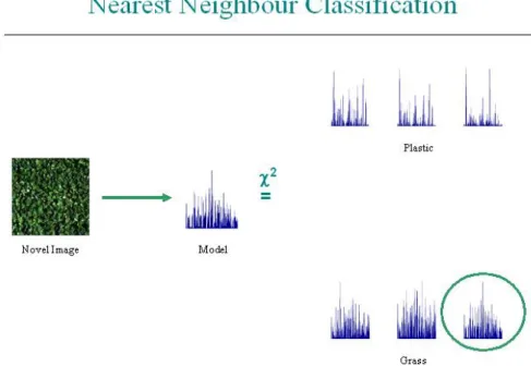
3.1.2 The Classification Stage

In the classification stage the different models learned from the training images are used to classify a novel image. The image to be classified is convolved with the MR8 filter bank. The filter

(31)

3.2 Image Patch Based Classifiers 13 responses allow the pixels labeling using the euclidean distance of each response to the textons in the texton dictionary. Once all image pixels are labelled the normalized frequency histogram defines the texture model. A nearest neighbor classifier is used to classify the new image using the

χ2_{statistic to measure the distance between two normalized frequency histograms.}

Figure 3.3: Nearest Neighbour classification

3.2 Image Patch Based Classifiers

The filter responses resulting from the convolution of the image with the filter bank can be seen as an inner product between image patch vectors and the filter bank matrix. The filter response can be considered as a lower dimensional projection of an image patch into a linear subspace [7].

3.2.1 Joint Classifier

The Joint classifier is similar to the VZ algorithm but instead of generating filter responses from a filter bank the pixel intensities of a N × N neighbourhood around the pixel are taken and row reordered to form a vector in a N2_{dimensional feature space.}

In the learning stage all the image patches from the training image are reordered, aggregated and clustered. The Texton dictionary is formed by the cluster centres, the textons now represent exemplar image patches rather than exemplar filter responses. The histogram of texton frequencies is used as the texture model. As in the VZ classifier the classification is achieved by nearest

(32)

14 The Varma-Zisserman Classifier

Figure 3.4: Classification without filtering

If we consider that textures can be realisations of Markov random field (MRF) two different variants of Joint Classifier can be designed. In a MRF the probability of the central pixel depends only on its neighbourhood.

p(I(xc)|I(x),∀x )= xc) = p(I(xc)|I(x),∀x ∈ N (xc))

Where xc is the central pixel and N (xc) is the neighbourhood of that pixel. Is this case, N

is defined as the N × N image patch, excluding the central pixel. Although the central pixel value is significant, its distribution is conditioned on its neighbours. To evaluate the significance of this conditional probability in classification the Neighbourhood an MRF classifiers were designed.

3.2.2 Neighbourhood Classifier

The Neighbourhood classifier is essentially the Joint classifier where the central pixel is discarded and only the neighbourhood is used for classification. The Joint classifier is retrained on features vectors drawn from the N × N image patches with the central pixel left out.

3.2.3 Markov Random Field Classifier

The MRF classifier models the joint distribution of the central pixels and its neighbours, p(I(xc),I(N (xc))).

The texton representation is modified to make explicit the central pixels PDF and to represent it in a finer resolution than its neighbours. The MRF texture model is the joint PDF represented by the matrix SN× SC, for each of the SN textons a one dimensional distribution of the central pixels

(33)

3.2 Image Patch Based Classifiers 15 intensity is learnt and represented by an SCbin histogram. The PDF of the central pixel for given

texton is represented by each row. The classification of the novel image is made by comparing the MRF distributions of the new model with learnt models using theχ2_{statistic over all elements of}

(34)

(35)

Chapter 4

Creating the Database

The first step of the project was collecting a set of masonry pictures to be tested with the chosen classifiers. The first set of images were given by Laboratório de Engenharia Sísmica e Estructural (LESE). Another set of masonry images was collected from the outskirts of Faculdade de Engen-haria da Universidade do Porto. And a third set of masonry images was downloaded from the internet. All images were captured with a commercial digital camera, the illumination of the walls should be as much uniform as possible.

4.1 Single Texture Images

From each image patches were cropped corresponding to each of two classes. The first class was the mortar and the second was the stone. From the set given by the LESE ten patches of each class were cropped. The different patches were chosen according to:

• Spatial localisation: evenly sampled over the entire image. • Illumination: well and uniformly illuminated areas. • Color: constancy over the image.

A single texture database composed of ten images of stone and ten images of mortar from the four different masonry wall, a total of 80 texture images was created. This set was used in the firsts tests of the classifiers.

4.2 Images with Two Texture Classes

From all the wall images compiled a set of six images was cropped. In each image, stone an mortar were present, the patches cropped were chosen according to the texture of the different elements. Three patches of each class were cropped from the images according to the criteria presented. All the images were manually labelled with two classes.

(36)

18 Creating the Database

Figure 4.1: Single texture images

(37)

Chapter 5

Using the VZ Classifier on Masonry

Walls

This chapter describes the methodology used to evaluate the effectiveness of the chosen classifiers to solve the specific problem of distinguishing mortar from stone in masonry walls. The VZ classifier and its variations was chosen thanks to the results presented [4] in the classification of single texture images.

This classification methodology used Matlab to create the different modules for the different stages. Matlab was chosen thanks to its variety of image processing functions present on the toolbox, also the possibility in integrating matlab scripts with LabView. More details about the Matlab modules developed are presented in appendix.

5.1 Classifying Single Texture Images

To implement the learning and classification stages of the VZ classifier different modules were created and tested in single texture images. The four different classifiers were implemented, the VZ with MR8 filter bank, the joint, the neighbourhood, and the MRF. The first data set was used in this stage.

5.1.1 The Learning Stage

The MR8 filter bank used in the VZ classifier could not be applied due to the images dimensions. For the joint, neighbourhood, and MRF classifiers the features were extracted according to the neighborhood size wanted. The Texton Dictionary for each classifier was obtained by clustering using kmeans. Each dictionary had ten textons. Each image pixel was classified by measuring the Euclidean distance to each texton in the dictionary, the pixel was labelled with the closest texton, creating a texture model according to the classifier and the neighborhood size.

(38)

20 Using the VZ Classifier on Masonry Walls

5.1.2 The Classification Stage

In the Classification stage the model of the image to be classified was created using the dictionary correspondent to the classifier chosen. Thenχ2_{distance between the new model and the training}

models was calculated. The image is classified according to the closest neighbour.

5.1.3 Results

The classifiers were applied to 80 texture images, 20 images from each class cropped from 4 different walls. The results obtained were close to the expected. The following table shows the classification accuracy for the experiment proposed using different classifiers.

N=3 N=7 N=9 Joint 78,75% 80% 78,75% Neighbourhood 76,25% 78,75% 78,75% MRF 87,50% 78,75% 87,5%

Table 5.1: Single texture classification results

Analysing the results we can observe that the results of the joint and neighbourhood classifier are very close, as expected. Curious is the fact that for N=7 the best classifier is the Joint classifier. As expected the best results are achieved with the MRF classifier using a N=9.

5.1.4 Conclusions

The classification results of the compiled database go in agreement with the expected values pre-sented in [4]. These results guarantee that the implemented classifiers were working as they should and can be used in future implementations.

5.2 Classifying Images with Two Texture Classes

After analysing the classification rates on single texture images the classifiers were applied on images with the two classes. From each image three different patches of each class were cropped and used in the learning stage of the classifiers. Texture models and the MR8 filter bank were not used due to the borders between classes. The image pixels were classified according to the texton dictionaries created in the learning stage.

5.2.1 Results

The images presented show the results of the pixel classification of three different images contain-ing the classes. In the first the stone pixels are clearly defined in white, although there are some

(39)

5.3 Evaluating the Dictionaries Quality 21

(a) Image 1 Accuracy Rate: 92,24% (b) Image 2 Accuracy Rate: 85,77%

(c) Image 3 Accuracy Rate: 58,85%

Figure 5.1: Different classification results

pixels clearly not classified correctly. The second shows a poorer classification but the stones and mortar are distinguishable. In the third case the classification is disastrous and the two classes are not distinguishable.

5.2.2 Discussion

Analyzing the results we see than the method is not very robust. In seems to work when the two classes have clearly different colors and textures. When the texture is similar and the color different it is still able to classify with a good accuracy rate. The error rate grows when the two elements are visually very similar. The confusion matrices of the results are presented in appendix ??.

5.3 Evaluating the Dictionaries Quality

Sometimes mortar and stone are very identical almost indistinguishable even for the human eye. The texture properties are very identical which becomes a challenge to the classifier. This proper-ties proximity will influence the quality of the dictionaries. The features space of the two dictio-naries becomes very close causing an increase of the error rate. A simple method was created to

(40)

22 Using the VZ Classifier on Masonry Walls

5.3.1 Texton Proximity

The Euclidean distance in feature space of each texton from the mortar dictionary to each texton from the stone is calculated, as well as the pair wise distance of the textons in each dictionary in order to evaluate the textons proximity.

Figure 5.2: Calculating distances between textons of different dictionaries, and pair wise distances In order to evaluate the dictionaries dispersion the minimum spanning tree was calculated. Given a connected, undirected graph, a spanning tree of that graph is a sub-graph which is a tree and connects all the vertices together. A weight can be assign to each edge, is this case the distance. A minimum spanning tree or minimum weight spanning tree is then a spanning tree with weight less than or equal to the weight of every other spanning tree. This result gives a quantification of the dispersion in the feature space of the texton dictionary.

(41)

Chapter 6

Discussion

In this chapter the most important contributions in this dissertation are summarized and a com-mentary on achievements is given. Finally, we also suggest possible directions and extensions for future work.

6.1 Commentary on achievements

The main achievements of this thesis were:

1. A database of labeled images of masonry walls with two different classes that can be used in future work aiming the same goal of this work. The images were collected with a com-mercial digital camera and hand labelled using a Matlab script.

2. A study of the ability of the VZ classifier to distinguish the different elements of a masonry structure. A methodology was implemented to test the quality of the textons dictionaries in classifying elements with similar textures.

3. Finally, all the methods were developed using Matlab scripts implemented and tested. This makes the future integration with LabView easier.

6.2 Conclusions

The goals purposed were not fully accomplished since a robust method able of distinguishing different types of stone and mortar with a reasonably low error rate was not achieved. On the other hand the first steps towards the resolution of a specific problem were given and we can take some conclusions.

To distinguish elements of similar texture the neighborhood features do not seem sufficient. Features other than color must be characterized and used as texture properties. In masonry struc-tures spatial distribution can be an important information source, able to give more information

(42)

24 Discussion

about the different elements. The information present in grey scale images does not sufficient to fully characterize the texture feature of the two classes.

6.3 Future Work and Extensions

A vital point that must be considered for future work is the use of the different color planes in order to get some spatial information. Analyzing the different planes can contribute with more in-formation both texture and spatial. Collecting and labeling more images will help the development of more accurate and robust classifiers.

Finally, the methods and Matlab modules implemented should be integrated with LabView. Once implemented, the classifiers can help in the study of structures and the creation of more accurate finite elements models, used in the evaluating the structural capacity of buildings.

(43)

Appendix A

Matlab Modules

To implement and study the different classifiers chosen it was used the Matlab environment due to the computational power, the existing image processing toolboxes and availability if different modules already developed for the implementations of the chosen classifiers.

In this section the principal modules created and implemented in the construction of the clas-sification algorithm are presented and briefly explained:

extract_features (I, N, classifier ): extracts all N × N from the grayscale image I and returns them as vectors according to the chosen classifier.

create_model (I, dic, classifier, N): returns the texture model of image I according to classifier, using dic as the texton dictionary.

dist_chi2 (A, B): returns the chi-square distance between model A and B.

test_dist (dic_A, dic_B): returns the minimum distances between different and pairwise textons, and the minimal spanning tree of each dictionary.

texton_atrib (I, dic): attributes to each pixel of I the closest texton of dic in the feature space. For more information on how the modules work or if you wish to download and use them contact: ee00032@fe.up.pt.

(44)

(45)

Appendix B

Confusion Matrices

The confusion matrices results of the two textures image classification are presented: Stone Mortar

Stone 253424 21836 Mortar 353 10183 Table B.1: Confusion Matrix Image 1

Stone Mortar Stone 387600 73140 Mortar 11836 124670 Table B.2: Confusion Matrix Image 2

Stone Mortar Stone 163025 415215 Mortar 125520 610204 Table B.3: Confusion Matrix Image 3

(46)

(47)

References

[1] www.masoncontractors.org. History of masonry.

[2] L. Binda, G. Cardani, A. Saisi, C. Modena, and M.R. Valluzzi. Multilevel approach to the analysis of the historical buildings: Application to four centers in seismic area finalised to the evaluation of the repair strengthening techniques. 13th Internationla Brick an block Masonry

Conference, July 2004.

[3] Wang Chen, Pau. The Handbook of Patern Recognition and Computer Vision. World Scien-tific Publishing Co., 2nd edition edition, 1998.

[4] Manik Varma and Andrew Zisserman. A statistical approach to texture classification from single images. International Journal of Computer Vision: Special Issue on Texture Analysis

and Synthesis, 2005.

[5] Daniel Di Capua and Laura Alvaresz Castells. Non-linear analysis of masonry walls using digital photography. 2002.

[6] National Instruments. NI Vision Concepts Manual, Junho 2008.

[7] Jasjit Suri Majid Mirmehdi, Xianghua Xie. Handbook of Texture Analysis. Imperial College Press, 2008.

[8] H. Tamura, S. Mori, and Y. Yamawaki. Textural features corresponding to visual perception.

IEEE Transactions on Systems, Man, and Cybernetics, SMC(8):460–473, 1978.

[9] J. Sklansky. Image segmentation and feature extraction. IEEE Transactions on Systems,

Man, and Cybernetics, SMC(8):237–247, 1978.

[10] R.M. Haralick. Statistical an structural approaches to texture. Proceedings of the IEEE, 67:786–804, 1979.

[11] W. Richards and A. Polit. Texture matching. Kybernetic, 16:155–162, 1974.

[12] P. Dewaele, P. Van Gool, and A. Oosterlinck. Texture inspection with self-adaptive convolu-tion filters. Proccedings of the 9th Internaconvolu-tional Conference on Pattern Recogniconvolu-tion, pages 56–60, Nov 1988.

[13] D. Chetverikov. Detecting defects in texture. Proccedings of the 9th International

Confer-ence on Pattern Recognition, pages 61–63, Nov 1988.

[14] J. Chen and A. K. Jain. A structural approch to identify defects in textured images.

Proceed-ings of the IEEE International Conference on Systems, Man, and Cybernetics, pages 29–32,

(48)

30 REFERENCES

[15] R. W. Conners, C. W. McMillin, K. Lin, and R. E. Vasquez-Espinosa. Identifying and locat-ing surface defects in wood: Part of an automated lumber processlocat-ing system. IEEE

TRans-actions on Pattern Analysis and Machine Intelligence, PAMI(10):92–105, 1983.

[16] R. Sutton and E.L. Hall. Texture measures for automatic classification of pulmonary disease.

IEEE TRansactions on Computers, C(21):667–676, 1972.

[17] H. Harms, U. Gunzer, and H. M. Aus. Combined local color texture analysis of stained cells.

Computer Vision, Graphics, and Image Processing, 33:364–376, 1986.

[18] A. Sousa. Analysis of colour and texture features of vital-stained magnification-endoscopy images for computer-assited diagnosis of precancerous and cancer lesions. Master’s thesis, Faculdade de Engenharia da Universidade do Porto, July 2008.

[19] K. Held, E. R. Kops, B. J. Krause, W. M. Wells, R. Kikinis, and H. Muller-Gartner. Markov random field segmention of brain mr images. IEEE Transactions on Medical Images, 16:878–886, 1997.

[20] M Ojala, M Pietikainen, and D. Harwood. A comparative study of texture measures with classification based on feature distributions. Pattern REcognition, 29, 1996.

[21] John A. Hartigan. Clustering algorithms. Wiley Series in Probability and Mathematical

Analysis and characterisation of masonry walls

F

E

U

P

Analysis and Characterisation of

Masonry Walls

Pedro Trigueiros de Sousa Pereira

Resumo

Abstract

Acknowledgments

Contents

List of Figures

List of Tables

Chapter 1

Introduction

1.1 Motivation

1.2 Goal of the work

1.3 Thesis Organization

Chapter 2

Texture Image Analysis

2.1 Digital Images

2.2 Image Textures

2.3 Common Applications

2.4 Review of Texture Analysis Methods

Feature

Formula

Energy

∑

∑

P

(i, j)

Entropy

−∑

∑

P

(i, j)logP

(i, j)

Contrast

∑

∑

(1 − j)

P

(i, j)

Homogeneity

∑

∑

Correlation

Chapter 3

The Varma-Zisserman Classifier

3.1 The Varma-Zisserman Classifier

3.2 Image Patch Based Classifiers

Chapter 4

Creating the Database

4.1 Single Texture Images

4.2 Images with Two Texture Classes

Chapter 5

Using the VZ Classifier on Masonry

Walls

5.1 Classifying Single Texture Images

5.2 Classifying Images with Two Texture Classes

5.3 Evaluating the Dictionaries Quality

Chapter 6

Discussion

6.1 Commentary on achievements

6.2 Conclusions

6.3 Future Work and Extensions

Appendix A

Matlab Modules

Appendix B

Confusion Matrices

References