Energy E¢ ciency and Price Regulation
Joisa Dutra
FGV, Centre for Regulation
Flavio M. Menezes
The University of Queensland
Xuemei Zheng
The University of Queensland
November 4, 2013
Abstract
This paper examines the incentives embedded across di¤erent regulatory regimes – price cap, rate of return and mandated target regulation – for investment in energy e¢ ciency programs at the supplier’s end of the network. In our model, a monopolist chooses whether or not to undertake an investment in energy e¢ -ciency, which is not observable by the regulator. We explore how the monopolist’s choice of e¤ort changes under di¤erent regulatory regimes. We show that, in equi-librium, the monopolist chooses to exert positive e¤ort more often under price cap regulation than under no regulation or mandated target regulation and that she exerts no e¤ort under rate of return regulation. In terms of expected welfare, however, the results are ambiguous and complex. In particular, we provide a full characterisation of the optimal e¤ort, optimal prices (regulated or unregulated) and expected welfare for the di¤erent regimes and show the trade-o¤s between rent extraction and incentives.
1
Introduction
Energy e¢ ciency programs have returned to the forefront of public policy. Such public interest in energy e¢ ciency programs had not been seen since their introduction in
Dutra and Menezes acknowledge the …nancial support of AusAid through an ALA Fellowship Award and FGV and Menezes also acknowledges the …nancial assistance from the Australian Research Council (ARC Grant 0663768). Zheng acknowledges funding from the China Scholarship Council and the University of Queensland.
the 1970s as a response to the oil shocks. Energy e¢ ciency is seen today as a cost-e¤ective approach to sustainable energy use and greenhouse gas emissions reductions. For instance, Metz (2001) argues that energy e¢ ciency improvement could potentially contribute to half of greenhouse emission reduction by 2020.
Despite their high pro…le, energy e¢ ciency opportunities have by and large not been materialised (Interlaboratory Working Group, 2000). This is particularly the case in the electricity sector where between 20 and 60 per cent of total electricity used could be conserved by cost e¤ective initiatives (Greenstone & Allcott, 2012). Although there are demand side management (DSM) programs1 that reduce consumption by a
kilowatt-hour at a cost lower than the cost of supplying that electricity, they are not widely used (Freeman et al. , 2010). There are several reasons why this may be the case. First, electricity suppliers (especially network service providers) need to invest in a range of infrastructure that is required to integrate distributed energy resources, including energy storage technologies, the digital hardware and software for improving transmission and distribution system reliability and security, and the supply-side and customer-side systems needed for full customer connectivity (Lester & Hart, 2012). Second, these …rms operate in a regulated environment where prices are usually set by a regulatory agency or government department that may not reward such investments by not considering them prudent or e¢ cient. Finally, investment in energy e¢ ciency may not be recouped if demand for electricity falls in the future or if the regulatory regime changes.
It follows then that electricity suppliers need to be incentivised to undertake energy e¢ ciency investment. Key policies promoting energy e¢ ciency in the electricity sec-tor include taxes, cap-and-trade systems and direct regulation of the …rms’operation. Creating incentives for suppliers/distributors to undertake energy e¢ ciency initiatives can be complex as these incentives interact with the form of price regulation. For example, in a context where …rms are allowed to recover, via prices, all the costs of sup-plying electricity to consumers, regulated …rms may have little incentive to undertake energy e¢ ciency investment. The interaction between price regulation and incentives for energy e¢ ciency is the subject of this paper.
In particular, we analyse the incentives for energy e¢ ciency embedded across dif-ferent regulatory regime – rate of return, price cap and mandated target regulation.
1DSM programs aim at both reducing consumers’ absolute electricity usage and shifting it from
peak to o¤ peak periods. Examples include enticements for consumers to acquire more energy e¢ cient electrical appliances and real time pricing of electricity consumption.
The interaction between price regulation and incentives for energy e¢ ciency is an im-portant public policy issue and the subject of this paper. We pursue this by building a theoretical model of a monopolist who can choose whether or not to undertake an investment in energy e¢ ciency. The investment is not observable by the regulator who can only determine whether the investment has been successful in terms of the level of energy e¢ ciency achieved. More speci…cally, the …rm’s choice of e¤ort a¤ects the probability of a successful outcome with a higher e¤ort resulting in a higher probability of achieving a better energy e¢ ciency outcome.
In this setting, regulatory regimes cannot explicitly compensate the …rm for the e¤ort it has put into energy e¢ ciency. We explore how di¤erent existing regulatory regimes perform in terms of expected amount of energy e¢ ciency and total welfare. In particular, we show, not surprisingly, that the monopolist chooses to exert e¤ort more often under price cap regulation than under no regulation and that she exerts no e¤ort under rate of return regulation. While we can show that price cap regulation dominates an unregulated monopolist in terms of expected welfare, the comparison between price cap and rate of return regulation, and between rate of return regulation and an unregulated monopolist, is ambiguous and complex. For example, when choosing low e¤ort is optimal regardless of the form of regulation, then price cap regulation always dominates an unregulated monopolist –both set prices ex-ante (that is, prior to the realisation of the energy e¢ ciency outcome) and prices are lower under price cap regulation.
The comparison between rate of return regulation and price cap regulation and that between rate of return regulation and no regulation are subtler. Rate of return regulation sets prices ex-post, conditional on the realisation of the energy e¢ ciency outcome, so that pro…ts are ex-post zero. This means that rate of return regulated prices can be either higher or lower than those under price cap regulation or no regulation. It follows that the regime which will yield the highest expected welfare will depend on demand, costs and the weight assigned by the regulator to the monopolist’s pro…ts in total surplus. We show, however, that mandated target regulation is always dominated by both price cap and rate of return regulation in terms of expected welfare although it can do better than an unregulated monopolist. The key reason is that mandated target regulation is too coarse and the trade o¤ between providing incentives to invest in energy e¢ ciency and rent extraction is less pronounced than under existing regulatory regimes such as price cap and rate of return regulation. More generally, we provide a full characterisation of the optimal e¤ort, optimal prices (regulated or unregulated)
and expected welfare for the di¤erent regimes and show the trade-o¤s between rent extraction and incentives.
This paper is organised as follows. Section 2 describes the key elements of the model. Section 3 develops the benchmark case of an unregulated monopolist’s choice of optimal e¤ort and pro…t-maximising quantity and price. In Section 4, we characterise outcomes under three distinct regulatory regimes, namely, rate of return, price cap and mandated target regulations. Section 5 compares the welfare under the di¤erent regulatory regimes, while Section 6 concludes.
1.1
Related Literature
Wirl (1995) examines the impact of regulation on DSM programs in a setting where electricity demand depends on service demand – the product of electricity usage and the energy e¢ ciency of the appliances. The regulated …rm aims to maximise pro…ts which are equal to the electricity sales revenue minus the electricity supply cost and investment in incremental energy e¢ ciency. Wirl (1995) shows that rate of return regulation fails to provide incentives for the …rm to undertake DSM. This is a direct result of the incentives that …rms regulated under rate of return regulation face to maximise total quantity sold (as the regulated price is greater than their incremental cost). Nevertheless, when combined with a shared savings mechanism, where the …rm is allowed to share some of the bene…ts accruing to consumers, rate of return regulation can lead to incentives for provision of DSM programs. The type of energy e¢ ciency program o¤ered by the regulated …rm, however, would favour high consumption rather than energy conservation. For example, the regulated …rm would favour programs with high rebound e¤ect –which refers to consumers’response to more e¢ cient appliances with more rather than less electricity consumption – such as providing more e¢ cient lighting and air conditioning. Doing so would result in consumers using more lighting in their gardens or setting lower temperatures in their living rooms.
In contrast, Wirl (1995) shows that, under price cap regulation, the regulated …rm may choose to invest in energy e¢ ciency at the consumer’s premises to mitigate the losses when consumers are sold electricity at below cost prices. Otherwise, the same issue as in rate of return regulation arises –a regulated …rm has an incentive to maximise quantity of electricity sold as long as the regulated price cap is above its incremental cost of supplying electricity. This suggests that to incentivise regulated …rms to invest in energy e¢ ciency requires decoupling revenue from quantity (Eto et al. , 1997; Brennan,
2010; Sullivan et al. , 2011). We also investigate the incentives embedded in di¤erent regulatory regimes but focus on energy e¢ ciency at the supplier’s end of the network rather than at the consumer’s side.
Eom (2009) and Chu & Sappington (2012) analyse a shared-savings incentive mech-anism for energy e¢ ciency programs with an energy saving target and investigate the design of a plan that maximises net social welfare. Chu & Sappington (2013) extend the analysis by considering a nonlinear reward structure. All the studies assume that e¤ort to provide energy e¢ ciency is unobservable by the regulator and take into account of impact of asymmetric information between the regulator and the regulated …rm in the provision of energy e¢ ciency programs. They suppose there is a positive relationship between e¤ort and the resulting energy e¢ ciency, and show that there is no simple, standard …nancial reward structure that will always induce the desired level of energy e¢ ciency e¤ort in all settings, as many factors may impact on the incentive mechanism, for instance, energy price, magnitude of rebound e¤ect and extent of observable energy e¢ ciency investment. In contrast, we examine the case where there is a probabilistic relationship between e¤ort and the actual amount of energy e¢ ciency achieved. This results in moral hazard and we investigate its impact on existing regulatory regimes rather than focus on the design of an optimal incentive scheme.
Finally, the existing literature on mandated targets focuses on standards for house-hold appliances (Daniel, 1980; Einhorn, 1982) and on the mandated quantitative targets for reducing energy use (Satchwell & Cappers, 2011; Brennan & Palmer, 2013; Palmer et al. , 2013). There are, however, very few analytical studies. Exceptions include Satchwell & Cappers (2011) and Brennan & Palmer (2013). Satchwell & Cappers (2011) analyse the …nancial impacts of the US Energy E¢ ciency Resource Standards (EERS) program on a speci…c regulated …rm, while Brennan & Palmer (2013) examine the economics of EERS by comparing with alternative measures such as energy taxes and cap-and-trade systems2. In contrast, we compare the power (and e¢ ciency) of the
incentives for energy e¢ ciency embedded in mandated target regulation with that of price cap and rate of return regulation.
2The study by Brennan & Palmer (2013) found that EERS is not an optimal option when the policy
goal is reducing energy use rather than reducing emissions. What’s more, an EERS could be optimal when marginal external harm falls with greater energy use.
2
The Model
We consider a monopolist that supplies electricity to …nal consumers. For simplicity, the demand function for electricity in the market is assumed to be linear, and the inverse demand function is given by:
P (Q) = a bQ; with a > 0; b > 0;
where Q denotes the amount of electricity that could be consumed by end users, and P is unit retail price of electricity. The monopolist can purchase wholesale electricity at a …xed price c > 0 and faces no …xed costs. In order to supply Q units of electricity to consumers the monopolist needs to purchase Qs units in the wholesale market. In
general, due to network losses, Q < Qs: By exerting e¤ort E = f0; eg the monopolist
can improve energy e¢ ciency by optimising the operation of the network3. In particular,
we denote by (E) = QQ
s the energy e¢ ciency parameter, which is a function of e¤ort
and can take two values 0 < < < 1. We assume that positive e¤ort implies a higher probability of achieving high energy e¢ ciency as detailed below.
We also assume that the cost of exerting e¤ort E is equal to E. Thus, the total cost of acquiring Qs units in the wholesale market and exerting e¤ort E is given by:
C(Qs; E) = cQs+ E:
It follows that the monopolist’s pro…t from selling Q units to …nal consumers is equal to
(Q; E) = P (Q)Q cQ
(E) E: (1)
Energy e¢ ciency is not a deterministic function of e¤ort and instead is determined according to the probabilities de…ned in Table 1.
Table 1: Relationship between e¤ort level and energy e¢ ciency
E = 0 1
E = e 1
We assume that > 12 so that as it is standard in moral hazard models the high level of e¤ort is more likely to lead to higher energy e¢ ciency than low level of e¤ort. Note
that the assumption that high energy e¢ ciency can eventuate even under zero e¤ort is a normalisation to simplify the characterisation of equilibrium behaviour. Without loss of generality, we assume a symmetric probability for energy e¢ ciency under the two the levels of e¤ort.
Given Table 1, the quantity of electricity the monopolist needs to purchase from the wholesale market is an expected value determined by the electricity price P and the e¤ort devoted to energy e¢ ciency E, which could be denoted as
Qs =
(
Qsl = Q +(1 )Q; E = 0
Qsh = (1 )Q + Q; E = e
: (2)
According to (2), the expected level of energy e¢ ciency is de…ned as
(E) = 8 < : l = (1 ) + ; if E = 0 h = +(1 ) ; if E = e ; (3)
with h > l by assumption. To insure an interior solution, we assume that:
a l c> 0; (4)
Consumer’s surplus is denoted by S(Q) and overall surplus by W (Q; E) = S(Q) + (P; E); where 0 < < 1 is the weight assigned by the regulator to the monopolist’s expected pro…t. The objective of the regulator is to maximise expected total surplus. As noted before, the regulator can observe the realisation of the level of energy e¢ ciency – for example, by monitoring both demand and the amount the electricity purchased by the supplier from the wholesale market, but not the level of e¤ort.
3
The Unregulated Monopolist
From 1, the unregulated monopolist’s expected pro…t can be rewritten as ( Qs; E) =
[a (E) c]Qs b[ (E)]2Q2s E. We can then calculate it by using (2) and (3):
( Qs; E) =
(
l= (a l c)Qsl b 2lQ2sl; E = 0 h = (a h c)Qsh b 2hQ2sh e; E = e
: (5)
@ l @Qsl = a l c 2b 2lQsl = 0; E = 0 @ h @Qsh = a h c 2b 2hQsh = 0; E = e
These FOCs yield that the optimal amount of electricity the monopolist purchases in the wholesale market is a function of e¤ort:
Qs = 8 < : Qsl= a l c 2b 2 l ; E = 0 Qsh = a h c 2b 2h ; E = e : (6)
The pro…t-maximising prices are then:
P = 8 < : Pl = a b lQsl = a l+c 2 l ; E = 0 Ph = a b hQsh = a h+c 2 h ; E = e : (7)
One can readily check that second-order conditions are satis…ed. We can replace (6) into (5) to obtain the maximised expected pro…ts as a function of e¤ort:
= 8 < : l = [a l c]2 4b 2 l ; E = 0 h = [a h c]2 4b 2 h e; E = e : (8)
We stress that the monopolist chooses a single price prior to the realisation of the energy e¢ ciency. Although the energy e¢ ciency outcome will be known by the time the electricity is used by consumers, we assume that the monopolist sells the electricity retail at a …xed price determined prior to the delivery of electricity.
3.1
Optimal Choice of E¤ort
In order to ensure that the monopolist remains in the industry the following participa-tion constraint needs to be satis…ed:
( Qs; E)> 0:
constraint, obtained directly from (8), needs to be satis…ed:
h l > 0:
Combining the participation and incentive compatibility constraints, we can now determine the unregulated monopolist’s optimal choice of e¤ort in Table 2:
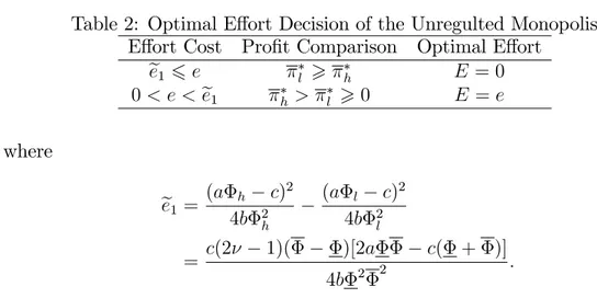
Table 2: Optimal E¤ort Decision of the Unregulted Monopolist E¤ort Cost Pro…t Comparison Optimal E¤ort
ee1 6 e l > h E = 0 0 < e <ee1 h > l > 0 E = e where ee1 = (a h c)2 4b 2 h (a l c)2 4b 2 l = c(2 1)( )[2a c( + )] 4b 2 2 :
Note that l > 0 given (8) and, therefore, the participation constraint is automati-cally satis…ed for both choices of e¤ort. That is, if the cost of positive e¤ort, e, is greater than the bene…t of the e¤ort (as measured by the di¤erence in expected pro…ts under the two e¤orts), then a zero e¤ort is optimal. Otherwise, the unregulated monopolist chooses to exert positive e¤ort. This is summarised in the following result. The proof is straightforward and, therefore, omitted.
Lemma 1 The unregulated monopolist chooses a positive level of e¤ort whenever 06 e < ee1: Otherwise she chooses zero e¤ort. The threshold value ee1 increases when the
demand shifts outward (i.e., a increases), or it becomes ‡atter/ less steep (i.e., b de-creases). The value of ee1 increases with c for su¢ ciently low values of c and decreases
with c for su¢ cient high values of c. Explicitly, ee1 decreases in c for c > a+ :
The e¤ort level chosen by the monopolist depends on expected values of energy e¢ ciency, shape of demand function (here it refers to the parameters a and b) and the wholesale price as well.
We now compute the social welfare in the absence of regulation: W (Q ; E) = bQ 2 2 + [P Q cQ (E) E] (9) = ( bQ 2 l 2 + l; E = 0 bQ 2 h 2 + h; E = e :
Given equations (6) and (8), we can rewrite the expected total social welfare under an unregulated monopoly for di¤erent levels of e¤ort as follows:
W = ( Wl = (2 +1)(a l c)2 8b 2 l ; E = 0 Wh = (2 +1)(a h c)2 8b 2 h e; E = e : (10) In the next section we investigate whether a welfare-maximising regulator may be able to improve upon (10) under di¤erent regulatory regimes.
4
Regulation and Energy E¢ ciency
This section investigates the incentives for energy e¢ ciency across three di¤erent types of regulatory regimes commonly observed around the world.
4.1
Rate of Return Regulation (ROR)
Under rate of return regulation, the regulator determines prices to cover the actual costs (including the cost of capital) incurred by the monopolist to supply electricity.4 In this
paper, we consider a stylised, pure form of rate of return regulation where the regulator observes both the actual electricity consumed (Q) and the electricity purchased by the monopolist (Qs): Therefore, the regulator can infer the level of energy e¢ ciency that
has eventuated although she cannot observe the e¤ort exerted by the monopolist. Note that this contrasts with how we model the unregulated monopolist who can only set prices ex-ante, prior to the realisation of the energy e¢ ciency outcome.
Prices then can take two values depending on the realised value of energy e¢ ciency, namely PROR if = and PROR if = : These values are calculated below but under such prices, the electricity purchased from the wholesale market is given by
4In practice, however, regulators typically attempt to ensure that incurred costs are e¢ cient. See,
either QsROR = a P ROR b if = or Qs ROR = a PROR b if = :As P
ROR and PROR are
…xed ex-post and do not depend on the monopolist’s e¤ort level, it can be easily checked that ROR(Q; e) ROR(Q; 0) = e < 0 for both realisations of and, therefore, we
have established:
Lemma 2 The monopolist always chooses to exert zero e¤ort under rate of return regulation.
We now turn our attention to determining the optimal ex-post regulated prices under rate of return regulation. As the weight given to the pro…ts of the monopolist is less than one, the regulator will set PROR so that pro…ts are zero. That is:
PROR = 8 < : PROR = c, = PROR = c; = : (11)
The next proposition summarises the outcomes under rate of return regulation including social welfare which is equal to expected consumer’s surplus given that the monopolist earns zero pro…ts.
Proposition 1 Under rate of return regulation, the monopolist chooses E = 0, and regulated prices are given by (11), and expected social welfare is given by:
Wror = (a c) 2 2b 2 + (1 )(a c)2 2b 2 :
4.2
Price Cap Regulation
Under our stylised form of price cap regulation, the regulator sets an ex-ante price –that is, a …xed price that is not conditional on the realised quantum of energy e¢ ciency –in order to maximise expected social surplus. In doing so, the regulator faces a trade-o¤ between providing incentives for energy e¢ ciency and reducing the monopolist’s rent. In particular, the regulator solves the following problem
M ax(Ppc)Wpc = Spc+ (Ppc; E)
s:t: (Ppc; E)> 0:
This problem is solved in several steps. First, we identify the optimal price cap as a function of e¤ort. We then determine the socially optimal level of e¤ort under the
optimally determined price cap. Finally, we combine these two steps to fully specify the solution to the problem above, that is, an ex-ante …xed price and the optimal level of e¤ort, as a function of various parameters including the cost of e¤ort. The …rst step is completed in the following Lemma. The proof is in Appendix A.
Lemma 3 The optimal price cap, as a function of e¤ort, is given by:
Ppc = 8 < : c l; E = 0 a h+c p(a h c)2 4b 2he 2 h ; E = e :
We now turn our attention to determine the optimal e¤ort from a monopolist who, in equilibrium, will face one of the two …xed prices above. If the price cap is set at c
l,
the monopolist’s expected pro…t is equal to:
pc = Ppc Q cQ (E) E = Ppc (a Ppc ) b c(a Ppc ) b (E) E = 8 < : pc l = c l(a c l) b c(a c l) b l = 0; E = 0 pc h = c l(a c l) b c(a c l) b h e; E = e ;
and, therefore, the incentive compatibility constraint can be written as:
pc h pc l = c(a l c)( h l) b h 2l e:
Similarly, if the price cap is set at a h+c p(a h c)2 4b 2he
2 h , the monopolist’s expected
pro…t is equal to:
pc = Ppc Q cQ (E) E = 8 < : pc l < 0; E = 0 pc h = 0; E = e ;
which implies that the incentive compatibility constraint, pch pcl > 0; is always satis…ed and the monopolist chooses to exert positive e¤ort at this ex-ante price. Proposition 2 The optimal price cap, level of e¤orts and expected social welfare are fully characterised in Table 3:
where
ee2 =
c(a l c)( h l)
b h 2l
Table 3: Characteristics of Price-cap Regulation
E¤ort Cost E¤ort Level Optimal Price Cap Expected Social Welfare e> ee2 E = 0 cl (a l c)2 2b 2 l 0 < e <ee2 E = e a h+c p(a h c)2 4b 2he 2 h (a h c)2+(a h c)p(a h c)2 4b 2he) 4b 2 h e 2
Note that the threshold value under price cap regulation is higher than that in the absence of regulation, i.e.,
ee2 ee1 =
c( h l)[2a l(2 h) + c( h+ l 4)]
4b 2 l h
> 0
Hence, the regulated …rm exert high e¤ort more often than under no regulation. The intuition for this is that under price cap regulation, the regulator sets a price ex-ante so that expected pro…ts are zero. The regulator anticipates the optimal e¤ort for the value of the cost of e¤ort and ensures that the monopolist is incentivised to put in positive e¤ort in situations where an unregulated monopolist would choose zero e¤ort. Thus, the range of values of the cost of e¤ort for which is worthwhile from a society’s perspective to engage in positive e¤ort is larger under price cap regulation than under unregulated monopoly.
In the same vein as ee1; it can be checked that ee2 is also increasing in a, decreasing
in b and either increasing or decreasing in c depending on its value.
It is worth noting that in our setting there is no meaningful distinction between price cap and revenue cap regulation. The optimal revenue cap can be implemented by the optimal price cap, which will result in the same expected revenue and welfare given that the demand function is deterministic. For completion, we spell out in the next Lemma what that optimal revenue cap is with associated calculations provided in Appendix A.
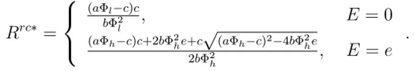
Lemma 4 The optimal revenue cap, as a function of e¤ort, is given by:
Rrc = 8 < : (a l c)c b 2 l ; E = 0 (a h c)c+2b 2he+cp(a h c)2 4b 2he 2b 2 h ; E = e :
4.3
Mandated Target Regulation
Mandated targets for achieving energy e¢ ciency have become widespread. For example, in the European Union there is a target of 20% improvement in energy e¢ ciency (as well as a 20% share of energy consumption from renewable resources) to be achieved by 20205. Under this approach, the regulator sets a minimum percentage of the energy
needs that have to be met through energy e¢ ciency programs. In our model we capture this regulatory approach by assuming that the regulator sets a target, mt;that needs to achieve in order to avoid a penalty > 0 for not meeting the target.
In this setting, the objective of the regulator is to set the target in order to maximise expected welfare subject to the …rm’s participation constraint:
M ax( mt)Wmt = Smt+ ( mt; E)
s:t: ( mt; E)> 0:
In our setting there are only two possible meaningful targets, namely or : If the mandated target is set at mt = , it is of course not binding and the monopolist’s expected pro…t is identical to the case of an unregulated monopolist and given by:
mt( mt; E) = ( P (Q)Q cQ l; E = 0 P (Q)Q cQ h e; E = e = P (Q)Q cQ (E) E; and the expected social welfare is
Wmt( mt = ) = bQ
2
2 + P (Q)Q
cQ
(E) E: With mt= as a target, the monopolist’s expected pro…t is
mt = ( P (Q)Q cQ l ; E = 0 P (Q)Q cQ h e (1 ) ; E = e = ( mt l = (a l c)Qsl b 2lQ2sl ; E = 0 mt h = (a h c)Qsh b 2hQ2sh e (1 ) ; E = e : 5http://ec.europa.eu/clima/policies/package/
The …rst-order conditions (FOCs) are respectively @ mtl @Qsl = a l c 2b 2lQsl = 0; E = 0 @ mth @Qsh = a h c 2b 2hQsh = 0; E = e
It follows that optimal electricity supply chosen by the monopolist and the related electricity price are identical with the associated levels under unregulated situation. Given this, the mandated target regulated monopolist’s expected pro…t is calculated as: mt = 8 < : mt l = (a l c)2 4b 2 l ; E = 0 mt h = (a h c)2 4b 2 h e (1 ) ; E = e :
The threshold value of e¤ort cost for energy e¢ ciency is
ee4 = (a h c)2 4b 2 h (1 ) (a l c) 2 4b 2 l + = (a h c) 2 4b 2 h (a l c)2 4b 2 l + (2 1) =ee1+ (2 1) >ee1:
That is, the range of e¤ort cost for which the monopolist …nds it worthwhile to exert positive e¤ort is larger than that for the unregulated monopolist. This is because by exerting positive e¤ort, the monopolist may avoid paying the penalty for not achieving the target. It is worthwhile to note that to guarantee the monopolist’s participation constraint, the penalty should be limited to 6 [a l c]2
4b 2 l = e0; thus ee4 ee2 = [a h c] 2 4b 2 h [a l c]2 4b 2 l + (2 1) c(a l c)( h l) b h 2l < 0; (12)
which implies that if the …xed penalty is relatively low, the threshold value of e¤ort cost under mandated target regulation is lower than that under price cap regulation.
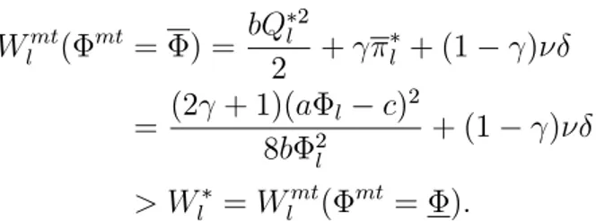
expected social welfare is Wlmt( mt= ) = bQ 2 l 2 + l + (1 ) = (2 + 1)(a l c) 2 8b 2 l + (1 ) > Wl = Wlmt( mt= ):
This is the same case with a relatively low e¤ort cost where positive e¤ort is cho-sen by the mandated target regulated …rm, i.e., Wmt
h ( mt = ) > Whmt( mt = ).
Therefore, the regulator’s optimal choice of mandated target is mt= .
The next proposition summarises the analysis above.
Moreover, compared with the non-regulated circumstance, mandated target regula-tion contributes to increase expected social welfare, no matter at which level the target is set.
Proposition 3 The optimal mandated target for energy e¢ ciency is mt = : The
characterisation of mandated target regulation is summarised in Table 4:
Table 4: Characterisation of Mandated-target Regulation
Mandated Target E¤ort Cost E¤ort Level Expected Social Welfare
mt = e> ee 4 E = 0 (2 +1)(a l c)2 8b 2 l + (1 ) 0 < e < ee4 E = e (2 +1)(a h c) 2 8b 2 h e + (1 )(1 )
5
Expected Welfare under Di¤erent Regulatory Regimes
This section compares the di¤erent regimes from an expected welfare perspective. The comparison is driven by the size of the cost of e¤ort. In particular, for e > ee2; the
monopolist chooses zero e¤ort under all possible scenarios. In this case, price cap regulation always dominates an unregulated monopolist –both set prices ex-ante (that is, prior to the realisation of the energy e¢ ciency outcome) and prices are lower under price cap regulation. This particular ranking is of course true for any cost of e¤ort as a regulator could always choose the unregulated monopolist’s price if it were to increase welfare.
Moreover, rate of return regulation performs better than price cap regulation when zero e¤ort is optimal. In this case, it is not necessary to incentivise the …rm to exert e¤ort into energy e¢ ciency and rate of return regulation then ensures that pro…ts are ex-post zero whereas under price cap regulation pro…ts are only zero ex-ante so prices are higher to ensure that the …rm’s participation constraint is satis…ed.
At the other extreme, when the cost of e¤ort is su¢ ciently low (that is, e < ee4);
price cap regulation always dominates rate of return regulation as it is socially optimal to set an ex-ante price that whilst ensuring that the …rm’s participation constraint is satis…ed, might result in positive (ex-post) pro…ts for the regulated …rm. At this price the …rm is incentivised to exert e¤ort in energy e¢ ciency. For intermediate values of the cost of e¤ort, the comparison between rate of return and price cap regulation is more complex as characterised in proposition 4 below.
Finally, we have shown that mandated target regulation is always dominated by both price cap and rate of return regulation in terms of expected welfare although it can do better than an unregulated monopolist. The key reason is that mandated target regulation is too coarse and the trade o¤ between providing incentives to invest in energy e¢ ciency and rent extraction is less pronounced. These results are summarised in the next proposition and its proof is in Appendix B.
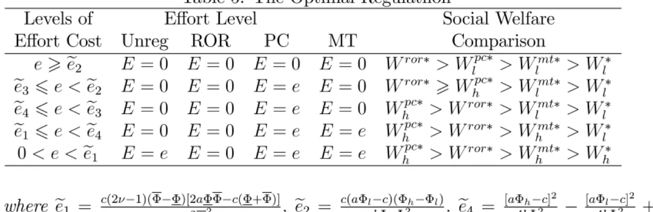
Proposition 4 The comparison of expected social welfare under di¤erent regulatory regimes is summarised in Table 5:
Table 5: The Optimal Regulatlion
Levels of E¤ort Level Social Welfare E¤ort Cost Unreg ROR PC MT Comparison
e> ee2 E = 0 E = 0 E = 0 E = 0 Wror > Wlpc > Wlmt > Wl ee3 6 e < ee2 E = 0 E = 0 E = e E = 0 Wror > Whpc > Wlmt > Wl ee4 6 e < ee3 E = 0 E = 0 E = e E = 0 Whpc > Wror > Wlmt > Wl ee1 6 e < ee4 E = 0 E = 0 E = e E = e Whpc > Wror > Whmt > Wl 0 < e <ee1 E = e E = 0 E = e E = e Whpc > Wror > Whmt > Wh where ee1 = c(2 1)( )[2a c( + )] 4b 2 2 ; ee2 = c(a l c)( h l) b h 2l ; ee4 = [a h c]2 4b 2 h [a l c]2 4b 2 l + (2 1) ; and ee3 denotes the point at which level of e¤ort cost Whpc = Wror :
6
Conclusion
This paper develops a theoretical model to investigate the relationship between a reg-ulated …rm’s incentive to invest in energy e¢ ciency and the nature of the regulatory regime. In this paper, the reason for the regulated monopolist not to undertake invest-ment in energy e¢ ciency is not due to her desire to maximise quantity but rather due to the inability of a regulator to commit to reimburse the e¤ort costs given that these are not directly observable. This is another channel through which regulatory regimes can disincentivise regulated …rms to invest in energy e¢ ciency – in addition to the issue of decoupling that was described in the introductory section. Price cap, rate of return and mandated targets deal with these lack of incentives in di¤erent ways. Rate of return provides no incentive to invest in energy e¢ ciency. Even if successful, the ex-post nature of rate of return regulation ensures that the …rm earns zero economic pro…ts. Price cap, in contrast, provides incentives for investment in energy e¢ ciency as the …rm is able to capture, in the event that the investment is successful, some of the economic rents. Mandate target regulation also provides incentives to invest in energy e¢ ciency by penalising the …rm for not achieving its target.
Our analysis suggests two key messages that might be of relevance to policy makers. First, when the cost of e¤ort to undertake energy e¢ ciency investment is low –that is, when there are existing opportunities that can be pursued at low cost and that are likely result in energy savings –a price cap regime is likely to perform better than a rate of return regulatory regime. Conversely, when the cost of e¤ort is too high, rate of return regulation is welfare superior to price regulation as in this instance it is not optimal for the …rm to invest in energy e¢ ciency. Second, mandated target regulation is clearly an inferior policy to stimulate investment in energy e¢ ciency. The key reason is that mandated target regulation is too coarse as an instrument to provide the appropriate incentives to the regulated …rm.
References
Brennan, Timothy J. 2010. Decoupling in electric utilities. Journal of Regulatory Economics, 38(1), 49–69.
Brennan, Timothy J., & Palmer, Karen L. 2013. Energy e¢ ciency resource standards: Economics and policy. Utilities Policy, 25(0), 58 –68.
Chu, LeonYang, & Sappington, David E. M. 2012. Designing optimal gain sharing plans to promote energy conservation. Journal of Regulatory Economics, 42(2), 115–134. Chu, LeonYang, & Sappington, David E.M. 2013. Motivating energy suppliers to
pro-mote energy conservation. Journal of Regulatory Economics, 43(3), 229–247.
Daniel, Khazzoom, J. 1980. Economic Implications of Mandated E¢ ciency in Standards for Household Appliances. The Energy Journal, 1(4).
Einhorn, Michael. 1982. Economic Implications of Mandated E¢ ciency Standards for Household Appliances: An Extension. The Energy Journal, 3(1), 103–109.
Eom, Jiyong. 2009. Incentives for utility-based energy e¢ ciency programs in California. Stanford University. Ph.D.
Eto, Joseph, Steven, Stoft, & Timothy, Belden. 1997. The theory and practice of decoupling utility revenues from sales. Utilities Policy, 6(1), 43 –55.
Freeman, Luisa, Intorcio, Shawn, & Park, Jessica. 2010 (March). Implementing En-ergy E¢ ciency: Program Delivery Comparison Study. IEE Whitepaper. Institute for Electric E¢ ciency.
Greenstone, Michael, & Allcott, Hunt. 2012. Is there an Energy E¢ ciency Gap? The Journal of Economic Perspectives, 26(1), 3–28.
Interlaboratory Working Group. 2000 (November). Scenarios for a Clean Energy Fu-ture. Report. Lawrence Berkeley National Laboratory, National Renewable Energy Laboratory and Oak Ridge National Laboratory.
Joskow, Paul L. 1974. In‡ation and Environmental Concern: Structural Change in the Process of Public Utility Price Regulation. Journal of Law and Economics, 17(2), 291–327.
Joskow, Paul L., Bohi, Douglas R., & Gollop, Frank M. 1989. Regulatory Failure, Regulatory Reform, and Structural Chang. Brookings Papers on Economic Activity, 125–208.
Lester, Richard K., & Hart, David M. 2012. Unlocking energy innovation: how America can build a low-cost, low-carbon energy system. Cambridge, Mass: MIT Press.
Metz, Bert. 2001. Climate change 2001: mitigation : contribution of Working Group III to the third assessment report of the Intergovernmental Panel on Climate Change. Cambridge: Cambridge University Press.
Palmer, Karen L., Grausz, Samuel, Beasley, Blair, & Brennan, Timothy J. 2013. Putting a ‡oor on energy savings: Comparing state energy e¢ ciency resource standards. Utilities Policy, 25(0), 43 –57.
Satchwell, Andrew, & Cappers, Peter. 2011. Carrots and sticks: a comprehensive business model for the successful achievement of energy e¢ ciency resource standards. Utilities policy, 19(4), 218–225.
Sullivan, Dylan, Wang, Devra, & Bennett, Drew. 2011. Essential to Energy E¢ ciency, but Easy to Explain: Frequently Asked Questions about Decoupling. The Electricity Journal, 24(8), 56 –70.
Wirl, Franz. 1995. Impact of regulation on demand side conservation programs. Journal of Regulatory Economics, 7(1), 43–62.
Appendix
Appendix A
Price Cap Regulation
The associated Lagrangian function for price-cap regulation is given by:
Lpc = (a P pc)2 2b + ( + pc)[Ppc(a Ppc) b (a Ppc)c b (E) E] = (a
2 2aPpc+ Ppc2) + 2( + pc)[(a + c)Ppc Ppc2 ac]
2b ( +
pc)E;
where pc> 0 is the Lagrangian multiplier. The Kuhn-Tucker conditions are
@Lpc @Ppc = (Ppc a) + ( + )(a + c 2 Ppc) b 6 0; P pc > 0; and Ppc@Lpc @Ppc = 0; @Lpc @ = (a Ppc)(Ppc c) b E > 0; pc > 0 and pc @Lpc @ pc = 0;
from which we identify three possible solutions: 8 < : P1pc = a +c2 p (a c)2 4b 2E 2 pc 1 = a c 2p(a c)2 4b 2E + 1 2 ; (13) 8 < : P2pc = a +c 2 + p (a c)2 4b 2E 2 pc 2 = a c 2p(a c)2 4b 2E + 1 2 ; or ( P3pc = ( (21)a + c1) pc 3 = 0
The participation constraint pc(Ppc; E) > 0 implies that P1pc 6 Ppc 6 P2pc with P1pc = a +c2 p (a c)2 4b 2E 2 and P pc 2 = a +c 2 + p (a c)2 4b 2E
2 . We can readily check
that P3pc does not satisfy the participation constraint as: pc(Ppc
3 ; E) =
( 1)(a c)2
(1 2 )2b 2 E < 0:
To select between P1pc and P2pc ;we compute the expected welfare associated with each price, W1pc and W pc 2 ;respectively, as follows: W1pc W2pc = (a P pc 1 )[(a P pc 1 ) + 2 (P pc 1 c)] 2b (a P2pc )[(a P2pc ) + 2 (P2pc c)] 2b = (2a 2a + 2 c)(P pc 1 P pc 2 ) (2 1)(P pc 2 1 P pc 2 2 ) 2b = (a c) p (a c)2 4b 2E 2b 2 > 0 (from 4)
It follows that the optimal price cap is Ppc = a +c2 p
(a c)2 4b 2E
2 :
Revenue Cap Regulation
Under revenue-cap regulation, the Lagrangian function of the welfare maximisation problem could be written as
Lrc= (a p a2 4bRrc)2 8b + ( rc+ )(Rrc c(a p a2 4bRrc) 2b (E) E);
and the Kuhn-Tucker conditions (KTCs) are @Lrc @Rrc 6 0; R rc> 0; and Rrc@Lrc @Rrc = 0; @Lrc @ rc = R rc c(a p a2 4bRrc) 2b E > 0; rc > 0 and rc @L rc @ rc = 0:
From the KTCs we get three sets of solution, i.e., 8 > < > : Rrc 1 = c2+ac +2b 2E cp(a c)2 4b 2E 2b 2 rc 1 = a 2 c+(2 1) pa2 4bRrc 1 2(c pa2 4bRrc 1 ) ; 8 > < > : Rrc 2 = c2+ac +2b 2E+cp(a c)2 4b 2E 2b 2 rc 2 = a 2 c+(2 1) pa2 4bRrc 2 2(c pa2 4bRrc 2 ) ; or ( Rrc 3 = (a c)(c + a a ) b(1 2 )2 2 rc 3 = 0 :
Given the above, suppose the monopolist’s expected pro…t with Rrc
3 is rc3 ;we obtain rc
3 < 0: Hence, the third set of solution dose not satisfy the participation constraint rc> 0, and we just need to consider Rrc
1 and Rrc2 when identifying the socially optimal
revenue cap. Denote the social welfare related to Rrc1 and Rrc2 respectively with W1rc
and Wrc 2 ; then W1rc= (a c) 2 2b 2E (a c)p(a c)2 4b 2E 4b 2 ; W2rc= (a c) 2 2b 2E + (a c)p(a c)2 4b 2E 4b 2 :
As the expected welfare di¤erence between Wrc
1 and W2rc is
W2rc W1rc= (a c) p
(a c)2 4b 2E]
2b 2 > 0;
the optimal revenue cap is Rrc = Rrc2 = c
2+ac +2b 2E+cp(a c)2 4b 2E
2b 2 :
It is interesting to note that the prerequisite Rrc < R is satis…ed: Proof.
) (a c)2 4b 2E + 2cp(a c)2 4b 2E > 0 ) 2c2+ 2ac + 4b 2E 2cp(a c)2 4b 2E < a2 2 c2 ) c 2+ ac + 2b 2E + cp(a c)2 4b 2E 2b 2 < (a + c)(a c) 4b 2 ) Rrc < R
Appendix B
From (12), it could be found that the threshold values of e¤ort cost under di¤erent regulatory circumstances satisfyee1 <ee4 <ee2:In the following analysis, we will consider
four distinguished situations, i.e., e> ee2; ee4 6 e < ee2, ee1 6 e < ee4 and 0 < e <ee1:
Case 1: In the case where e > ee2; no positive e¤ort is taken by the monopolist
either under the unregulated situation or under any of the three types of regulation analysed above. The resulted expected social welfare under di¤erent regulatory circumstances are given as:
Wl = W (E = 0) = (2 + 1)(a l c) 2 8b 2 l ; Wror = Wror (E = 0) = (a c) 2 2b 2 + (1 )(a c)2 2b 2 ; Wlpc = Wpc (E = 0) = (a l c) 2 2b 2 l ; Wlmt = Wlmt (E = 0) = (2 + 1)(a l c) 2 8b 2 l + (1 ) : Then we can obtain the comparison as follows:
Wlpc Wror = (a l c) 2 2b 2 l (a c)2 2b 2 (1 )(a c)2 2b 2 = cv(1 )( ) 2 2b 2 2 < 0 ) Wlpc < W ror :
It could be found that in this case the expected social welfare under ROR regulation dominates that under price-cap regulation.
Moreover, Wlmt Wl = (1 ) > 0 Wlpc Wlmt = (a l c) 2 2b 2 l (2 + 1)(a l c)2 8b 2 l (1 ) > (a l c) 2 2b 2 l (2 + 1)(a l c)2 8b 2 l (1 ) (a l c)2 4b 2 l = (a l c) 2 8b 2 l > 0
To sum up, if the e¤ort cost is so high that no energy e¢ ciency e¤ort is undertaken under any scenario, i.e., when zero e¤ort is the optimal choice for the monopolist, the merit of expected social welfare brought about by these regulatory situations are given as
Wror > Wlpc > Wlmt > Wl
Case 2: In the case where ee4 6 e < ee2; only under price-cap regulation does
the monopolist have incentive to undertake positive e¤ort for energy e¢ ciency improvement, then under this circumstance the related expected social welfare are respectively: Wl = W (E = 0) = (2 + 1)(a l c) 2 8b 2 l ; Wror = Wror (E = 0) = (a c) 2 2b 2 + (1 )(a c)2 2b 2 ; Whpc = Wpc (E = e) = (a h c) 2+ (a h c) p (a h c)2 4b 2he 4b 2 h e 2; Wlmt = Wlmt (E = 0) = (2 + 1)(a l c) 2 8b 2 l + (1 ) : It could be seen that the comparison between Wl, Wror and Wmt
l is the same with
that in the case where e> ee2, thus we just need to compare W pc
h to Wl , W
ror and
As @Whpc @e = (a h c) 4b 2 h 4b 2 h 2p(a h c)2 4b 2he 1 2 = (a h c) 2p(a h c)2 4b 2he 1 2 < 0; we have Whpc Wlpc = (a h c) 2+ (a h c) p (a h c)2 4b 2he 4b 2 h e 2 (a l c)2 2b 2 l > (a h c) 2+ (a h c) p (a h c)2 4b 2hee2 4b 2 h ee2 2 (a l c)2 2b 2 l > 0;
thus it could be found that Whpc > Wlpc > Wmt
l > Wl .
As @W
pc h
@e < 0; we can, in the range ofee4 6 e < ee2; obtain that
Whpc (e =ee2) Wror < Whpc W ror < Wpc h (e =ee4) Wror Whpc Wror = (a h c) 2+ (a h c) p (a h c)2 4b 2he 4b 2 h e 2 (a c)2 2b 2 (1 )(a c)2 2b 2 ( > 0; if ee4 6 e < ee3 6 0; if ee3 6 e < ee2 ;
where Whpc = Wror at the point e = ee3: Therefore, in this case the comparison is
summarised in the following table.
e W ee4 6 e < ee3 Whpc > Wror > Wlmt > Wl ee3 6 e < ee2 Wror > W pc h > W mt l > Wl
positive e¤ort for energy e¢ ciency under both price-cap regulation and mandated-target regulation, then under the circumstance the relevant levels of expected social welfare are respectively:
Wl = W (E = 0) = (2 + 1)(a l c) 2 8b 2 l ; Wror = Wror (E = 0) = (a c) 2 2b 2 + (1 )(a c)2 2b 2 ; Whpc = Wpc (E = e) = (a h c) 2+ (a h c) p (a h c)2 4b 2he 4b 2 h e 2; Whmt = Wmt (E = e) = (2 + 1)(a h c) 2 8b 2 h e + (1 )(1 ) : As e <ee4 = [a h c] 2 4b 2 h [a l c]2 4b 2 l + (2 1) ;it is easy to obtain Wmt h > Wlmt :From the
previous analysis, we know that Wlmt > Wl :Therefore, Whmt > Wl: As Wror Whmt = (a c) 2 2b 2 + (1 )(a c)2 2b 2 (2 + 1)(a h c)2 8b 2 h + e (1 )(1 ) > (a c)2 2b 2 + (1 )(a c)2 2b 2 (2 + 1)(a h c)2 8b 2 h + ee1 (1 )(1 ) e1 = (a c) 2 2b 2 + (1 )(a c)2 2b 2 (2 + 1)(a h c)2 8b 2 h +2 (a h c) 2 8b 2 h (a l c)2 4b 2 l (1 )(1 )(a l c)2 4b 2 l = (a c) 2 2b 2 + (1 )(a c)2 2b 2 (a h c)2 8b 2 h (a l c)2 4b 2 l (1 )(1 )(a l c)2 4b 2 l = (a c) 2 2b 2 + (1 )(a c)2 2b 2 (a h c)2 8b 2 h [1 + (2 1) ](a l c)2 4b 2 l > (a c)2 2b 2 + (1 )(a c)2 2b 2 (a h c)2 8b 2 h (a l c)2 4b 2 l > 0; we have Wror > Whmt > Wl :
From the assumption that Whpc = Wror at the point e =ee
3 >ee4;it could be found
e¤ort cost e; it is safely to conclude that in this case Whpc > Wror :
Thus in this case, the comparison is summarised as Whpc > Wror > Whmt > Wl: Case 4: in the case where 0 < e < ee1; the monopolist is prone to undertake
positive e¤ort for energy e¢ ciency except under ROR regulation, then under the circumstance the relevant levels of expected social welfare are respectively:
Wh = W (E = e) = (2 + 1)(a h c) 2 8b 2 h e; Wror = Wror (E = 0) = (a c) 2 2b 2 + (1 )(a c)2 2b 2 ; Whpc = Wpc (E = e) = (a h c) 2+ (a h c) p (a h c)2 4b 2he 4b 2 h e 2 Whmt = Wmt (E = e) = (2 + 1)(a h c) 2 8b 2 h e + (1 )(1 ) From the analysis in the above three cases, we know Wmt
h > Wh: Thus in this case,
the comparison could be summarised as Whpc > Wror > Wmt