Environmental Regulation and Technological
Innovation with Spillovers
Samiran Banerjee and Jo˜ao E. Gata
∗June 23, 2004
Abstract
We present a two-period dynamic model of standard setting under asymmetric information to model the attempts by the Califormia Air Resources Board (CARB) in getting car manufacturers to comply with its phase-in of stringent emissions standards. After CARB chooses an initial emissions standard that firms are required to comply with, au-tomakers respond by choosing R&D investment and production levels which provide CARB an imperfect signal whether they are more or less capable of complying with the standard. CARB resets the en-vironmental standard and the firms once again choose research and production levels. Firms are Cournot duopolists in the product mar-ket and can choose to do research noncooperatively or cooperatively in the presence of spillovers. We show that firms will behave strategically and underinvest in research both under competitive and cooperative R&D, though the level of underinvestment — the ratchet effect — is greater under cooperative R&D when spillovers are large. We uncover a fundamental conflict between the incentives of firms to do cooper-ative research and social welfare: that firms will want to engage in cooperative (resp. noncooperative) R&D only when spillovers are low (resp. high) while social welfare is greater under noncooperative (resp. cooperative) research.
JEL Numbers: L5, O3
1
Introduction
Technology-forcing regulation is intended to correct market failures involving externalities by forcing firms to innovate, the underlying belief being that so-cially beneficial technologies might remain undeveloped or under-developed in a free market environment, especially if anticipated development costs exceed the private benefits of the developer at the margin. In the specific context of automobile emissions control in the U.S. which is our focus, the California Air Resources Board (CARB) in 1990 passed a stringent set of emissions standards which now cover over 40% of the US automobile market. But even though the California plan required auto manufacturers to produce and sell an increasing percentage of zero-emissions vehicles (ZEVs or electric cars),1
automobile companies have argued strenuously that these emissions targets are impossible to meet because of technological impediments.2
Over several years, CARB has had to successively relax its standards.3
Our ob-jective in this paper on the one hand is to model this market as an explicit dynamic game between car manufacturers and CARB; on the other, we
ex-1
These were 2% in 1998, 5% by 2001, 10% by 2003; the corresponding numbers for low emission vehicles were 48%, 90% and 95%, while for ultra-low emission vehicles were 2%, 5% and 15%. The low and ultra-low emission categories necessitate substantial im-provements in catalytic converter efficiency, the use of reformulated fuel and the use of alternative fuels such as methane and compressed natural gas, or hybrid (fuel and electric-powered) vehicles.
2
For instance, many viewed the launch of EV1 in 1996, General Motors’ electric car with its price tag of $35,000, a maximum speed of 80 mph, a running distance of 70-90 miles, and a recharging process of around 15 hours without a high-speed charger as an attempt to convince the regulators that the company was genuine in its attempt to meet the emission standard but that technological impediments made this impossible. SeeThe Economist, January 13, 1996.
3
plore the role of noncooperative and cooperative pre-competitive R&D in the presence of spillovers in meeting CARB’s regulatory objectives.
Our model is based on the classic paper on horizontal R&D of d’Aspr´emont and Jacquemin (1988) — henceforth D’A&J — and Yao’s (1988) model of standard setting under asymmetric information. We consider a duopoly of automakers and a regulator (CARB) facing a market demand where con-sumers are assumed to be willing to pay more for cars meeting higher emis-sions standards.4
Firms know their technological ability to comply with an emissions standard at a low or high cost (i.e., whether they are ‘low-cost’ or ‘high-cost’ types) but CARB does not. In the first period, CARB chooses an initial emission standard which the firms are required to comply with. Automakers respond by choosing R&D investment levels, followed by their production decisions which provide an imperfect signal to CARB regarding their types. Based on this signal, CARB resets the environmental standard at the beginning of the second period and the firms once again choose research and production levels. Firms can choose to do research noncooperatively or cooperatively in the presence of technological spillovers and are Cournot duopolists in the product market.
We find that low-cost firms will behave strategically and underinvest in research in the first period, both under competitive and cooperative R&D. The rationale for this is that by underinvesting, firms are able to preempt CARB from raising the emissions standard in the second period, leading to substantial gains in second period profits that more than compensate for lower first-period profits. The level of underinvestment (the ratchet effect)
4
is greater under cooperative R&D when spillovers are large. While it is to be expected that society’s goals may be at odds with private incentives in this setting — indeed, that is often the justification for technology-forcing regulation in the first place — we find that when spillovers are high, social welfare is greater when firms engage in cooperative R&D but firm profits are greater if they do not cooperate in research. Therefore if spillovers are high, firms may need additional inducement to engage in cooperative R&D.
Although Yao (1988) has also shown that when product standards are im-posed by regulation, car makers have the incentive to underinvest in R&D,5
our model differs significantly from his in several respects. In Yao’s work, the industry is modeled as a reduced-form entity whose only decision is how much to invest in R&D in both periods, and research success (i.e., low-cost compliance) is probabilistic. We consider a duopoly where each firm decides not only how much to invest in R&D in both periods, but also how much to produce in both periods within a Cournot framework since firms have to produce the cars meeting the current emissions standard in each period. Re-search, be it cooperative or non-cooperative, is deterministic. Furthermore, while Yao has a constant marginal benefit from the emissions standard, in our case cleaner cars are of additional value to consumers which changes the potential gains from trade (and hence the marginal benefit) as the standard changes. This marginal benefit is also affected by the strategic production de-cisions of the firms which determine the market equilibrium price, a channel of influence that is missing in Yao.
The paper is organized as follows. In Section 2 we describe the basic model, followed by a derivation of the full-information benchmark in Sec-tion 3. SecSec-tion 4 comprises the main results of the paper in analyzing the no-precommitment asymmetric information case. Section 5 presents a
pre-5
commitment and self-regulation scenarios. Conclusions and other comments are in Section 6.
2
The basic model
We model a two-period extensive form game with three players, CARB and two identical firms, i and j. In each period t, the firms face an inverse demand pt =a+ηt−(qi
t+q j
t), where pt is the output price,{qti, q j
t}denotes
the output produced by each firm, and ηt is an emissions or environmental standard chosen by CARB that increases the potential social surplus by shifting the demand curve outward — consumers value cars meeting higher emissions standards and are willing to pay more for them. The per-unit cost of production for firm i at time t is given by ci
t = kηt−xit−σx j t,
6
where
k ∈ {kL, kH} is a cost parameter (0 < kL < kH < 1) which reflects the inherent productive capability of a firm and influences how the emissions standard impacts costs, {xi
t, x j
t} are the research expenditures of both firms
which measures their R&D efforts and lowers their unit cost of production, andσ ∈[0,1] is an exogenously given research spillover parameter. Note that for any emission standard level η, a firm with a low k value (henceforth, a
low-cost firm) indicates a more productive firm capable of complying with the environmental standard at a lower per-unit production cost than a high-cost firm. Firms are both either low-cost or high-cost.
In each period t, and following Yao and D’A&J, a firm’s profit is given byπt= (pt−ct)qt−γ2x
2 t−
µ 2η
2
, where the second term on the righthand side reflect increasing research costs, and the third term is a fixed cost of attaining the prevailing emissions standard which increases with the standard. Firm
i (similarly, j) maximizes the discounted sum of two-period profits Πi = πi
1+δπ2i, whereδis a discount factor that is common to both firms and CARB. 6
Here and later, the corresponding derivation for firmj can be found by transposing
Henceforth, we will set δ = 1; the implications of relaxing this assumption are discussed in Section 5. Under noncooperative R&D, firms initially choose research levels non-cooperatively and subsequently compete `a la Cournot in the product market. Under cooperative R&D, firms first choose R&D levels so as to maximize joint industry profits and subsequently choose output levels noncooperatively.
Except under the full information scenario, we suppose that CARB can-not observek but believes that it is either low (kL) with probabilityθor high (kH) with probability (1−θ). The value ofθ is unknown but is believed to be uniformly distributed over the interval [0,1].7
At the end of the first period, CARB may choose to audit the first-period cost and update its prior regard-ing θ before setting the second period emission standard. CARB’s auditing effort is assumed to be costless.
Using this basic model, we start with a benchmark full information sce-nario followed by an asymmetric information scesce-nario, each under both non-cooperative and non-cooperative R&D. In the asymmetric information scenario which is the main focus of this paper, CARB sets a standard in the first pe-riod, gathers information on first-period costs and updates its prior on both firms’ type before setting a second period emission standard. In Section 5, we briefly discuss a precommitment scenario (when CARB is able to cred-ibly precommit to an emission standard which prevails for both periods at the start of the game) as well as a self-regulation scenario (when firms are allowed to cooperatively choose an emissions standard that applies to both periods, before knowing their true type).
7
More generally, one may assume that θ follows a beta distribution with parameters
3
Emissions standard under full information
3.1
Non-cooperative R&D
If CARB can observe k ∈ {kL, kH}, no updating is necessary and all time period subscripts can be dropped because the solution to the two-period problem is merely the solution to the one-period problem repeated twice. Given the chosen emission standardη, research levels{xi, xj}, and takingqj
as given, firm ichooses qi to maximize its profit function:
πi(qi, qj;xi, xj) = (p−c)qi− γ
2(x
i
)2 − µ
2η
2
wherep=a+η−(qi+qj) andc=kη−xi−σxj. The Nash equilibrium
out-put level of firmiis given by qi = [a+η(1−k) + (2−σ)xi+ (2σ−1)xj]/3.
Plugging the values of qi and qj into the profit function above yields a
reduced-form profit function, πi(xi, xj). Then, at the preceding stage, firm i chooses an R&D level by maximizing πi(xi, xj) with respect to xi.8
Solv-ing this maximization problem assumSolv-ing symmetry, each firm’s one-period Nash equilibrium research and production levels under noncooperative R&D (indexed by the superscript N) are given by:
xN = (2−σ)[a+η(1−k)]
D and q
N = 1.5γ[a+η(1−k)]
D , (1)
where D = 4.5γ −(2−σ)(1 +σ); we assume γ > 1 which ensures D > 0. Note that the output and research levels are higher if the firms are low-cost, i.e., if k=kL.
CARB’s objective is to maximize the one-period social surplus by choos-ing η appropriately. This second best surplus is simply the sum of consumer and producer surpluses at the aggregate output level QN, given by the Nash
equilibrium production levels, i.e., QN = 2qN. The one period social surplus
8
is then
WN(xN, QN, η) = QN
0
(a+η−Z)dZ−kη−(1 +σ)xNQN−γ(xN)2 −µη2
(2)
where the term under the integral is the area under the demand curve and all the other terms are aggregate costs of production and research.9
Making use of (1) and then maximizing WN(xN, QN, η) with respect to η yields:
ηN = aγ(1−k)A 2µD2
−(1−k)2
γA, (3)
where A= 18γ−2 (2−σ)2 >0 forγ >1.10
Note thatηN decreases with k,
i.e., the emission standard will be higher if both firms are low-cost (k=kL). Finally, each firm’s equilibrium profit level is given by:
πN = 1
9
a+ηN(1−k) + (1 +σ)xN2− γ
2(x
N)2 −µ
2(η
N)2
. (4)
3.2
Cooperative R&D
As in the previous case, firm i chooses qi non-cooperatively in the second
stage and similarly for firm j. But now, in the preceeding stage firms maxi-mize joint profitsπi(xi, xj)+πj(xi, xj) with respect toxiandxj, internalizing
the R&D spillovers. The one-period equilibrium solutions for research and production levels under cooperative R&D (indexed by the superscriptC) are given by:
xC = (1 +σ)[a+η(1−k)]
D′ and q
C
= 1.5γ[a+η(1−k)]
D′ , (5)
where D′ = 4.5γ−(1 +σ)2
>0. Note that D > D′ for σ >0.5, so for high spillovers both output and research levels are higher under cooperative than
9
Note that in this measure of social surplus, CARB takes the duopolistic market struc-ture as given, i.e., it corresponds to Suzumura’s (1992) ‘second-best welfare function’.
10
The second order sufficient condition is that the denominator ofηN
under non-cooperative R&D. Given the aggregate output level QC = 2qC,
CARB maximizes the one-period social surplus WC(xC, QC, η) with respect
to η, to obtain:
ηC = aγ(1−k)A ′ 2µ(D′)2
−(1−k)2
γA′ (6)
where A′ = 18γ−2(1 +σ)2
>0. Given the emissions standard ηC, each firm
will maximize its profit level πC(xC, qC, ηC).
3.3
Full information R&D, profit, and social welfare
The following two propositions follow from the derivations in the previous two subsections:
Proposition 1 Under full information and either noncooperative or coop-erative R&D, the output and research levels as well as the optimal emission standard will be higher for low-cost firms (i.e., k = kL) than for high-cost firms.
Proposition 2 Under full information and for any given firm type (kH or kL), a high level of research spillover (i.e., σ >0.5) implies a higher output and research level as well as a higher optimal emission standard under coop-erative R&D, as compared to non-coopcoop-erative R&D. A low level of research spillover (i.e., σ < 0.5) implies higher output and research levels as well as a higher optimal emission standard only under non-cooperative R&D.11
Proposition 1 is easy to understand: when firms are low-cost and therefore more productive, they produce more and undertake more research. It is also socially optimal to set a higher emission standard in this case since the marginal social cost of meeting this standard by low-cost firms is lower.
11
Regarding Proposition 2, when spillovers are low (i.e., σ < 0.5), and for any given emissions standard η, although an increase in a firm’s R&D investement, say firm i, will lower both firms unit production costs, it will lower firm i’s unit cost sufficiently more than firm j’s unit cost so as to give firm i a competitive edge over firm j in the output market, which is larger than the competitive edge firm i would obtain if spillovers were high. Hence, when spillovers are low, R&D investment and output levels are higher under non-cooperation than under cooperation. CARB will then set a higher standard η when spillovers are low and firms do not cooperate in R&D, because under this scenario firms tend to invest more in R&D than under the cooperative scenario. The reverse is true under the cooperative scenario.
Because of the complex interplay between R&D choice, output levels and the optimal emission standard, analytical results are very difficult to obtain; therefore, we have resorted to simulations to gain additional insights into this model. Our benchmark parameter values are γ = 5.5, kL = 0.45, kH = 0.6,
µ= 0.4, and with σ ranging between 0.33 and 0.9.12
Simulation Result 1 Under cooperative R&D, firm profits are higher when σ is low (e.g., for 0.33 ≤ σ < 0.5) and lower when σ is high (e.g., for
0.5< σ ≤0.9) relative to the non-cooperative R&D scenario, and regardless of whether both firms are high or low cost.
To understand this result, note that from Proposition 2, a low σ means a higher output level (and hence higher gross profits) under noncooperation, but the higher emission standard imposes a large enough cost that noncoop-eration profits are smaller than those under coopnoncoop-eration. Thus ifσ were low, firms would prefer cooperation over noncooperation. For analogous reasons, firms would prefer noncooperation over cooperation for a high σ.13
12
An Excel simulation file is available from the authors upon request. 13
Simulation Result 2 Under cooperative R&D, social welfare (and consumer surplus) is higher when σ is high (for 0.5 < σ ≤ 0.9) and lower when σ is low (for 0.33 ≤σ < 0.5) relative to the non-cooperative R&D scenario, and regardless of whether both firms are high or low cost.
The second simulation result indicates that even though firm profits are lower under cooperation when spillovers are high, the higher emission standard in-creases consumer surplus sufficiently that welfare levels are higher than under noncooperation. Hence, even though R&D cooperation is socially desirable in that it results in higher welfare, firms do not have an incentive to engage in it. This fundamental conflict between the private incentives of firms and what is socially desirable, even under full information, is an interesting and unique feature of our model with policy consequences: even if spillovers are high, firms may need external inducements in order to undertake cooperative R&D. It should be noted that this result is quite different from D’A&J where social and private incentives coincide.
4
Emissions standard without pre-commitment
4.1
Non-cooperative R&D
In this scenario, there is information asymmetry between the regulator, CARB, and the regulated firms. CARB cannot observe k but believes that it is either low (kL) with probability θ or high (kH) with probability (1−θ). The value of θ is unknown but is believed by CARB to be uniformly dis-tributed over the interval [0.1], i.e., at first, CARB presumes that kL and
kH are equally likely. But after observing the first-period cost, it updates its prior regarding θ. Under noncooperative R&D, the two-period problem consists of 6 steps as in Yao (1988):
1. CARB chooses η1 based on its prior about θ,
2. firms choosexi 1, x
j 1
3. firms choose qi 1, q
j 1
given η1 and
xi 1, x
j 1
,
4. CARB observes (audits) the cost c1 and chooses η2 based on updated
prior about θ,
5. firms choose xi 2, x
j 2
noncooperatively given η2, and
6. firms choose qi 2, q
j 2
given η2 and
xi 2, x
j 2
.
This sequence of moves resembles reality in two critical respects. First, as discussed in the introduction, the history of emission regulations shows that although regulations are initially imposed with a specific deadline, apparently CARB has not been able to credibly hold the firms to that deadline, and in practice the standards have been revised in a dynamic interplay between the concerned parties. This feature is captured in the two-period extensive form game outlined above. Second, the actual CARB mandates are phased in gradually and dynamically over a certain number of years, and our model reflects this in that the firms have to undertake the production of vehicles meeting the current environmental standard in each period.
The game is solved backwards for a perfect Bayesian equilibrium assuming that CARB is aware of the fact that the research and production levels by the firms are symmetric in equilibrium.
Steps 5 and 6. The calculation of second period output and research levels mirrors Section 3.1, where the values of ¯xN
2 and ¯q N
2 are given by equation
(1) with k =kH or kL (depending on the firms’ type), and η = η2. Second
period profits are given by equation (4) with appropriate substitutions.
costs, but it raises the unit production costs in order for CARB to be unable to distinguish them from high-cost firms. Thus first period profits are not necessarily lower; however, manipulation does reduce the the second period emissions standard and thereby raises second period profits. While we were unable to resolve analytically whether overall profits were greater or not, we could not find any parameter configuration where the following simulation result did not hold:
Simulation Result 3 Manipulation is a dominant strategy for low-cost firms for any positive discount factorδ, i.e., low-cost firms always have an incentive to manipulate their first-period costs.
When low-cost firms manipulate in the first period, CARB learns nothing regarding the firms’ true type and its prior unaffected. Consequently at the beginning of the second period in step 4, CARB choosesη2 so as to maximize
the expected social surplus
EWN 2 (¯x
N 2 ,Q¯
N
2 , η2) =E Q¯N2
0
(a+η2−Z)dZ−kη2−(1 +σ)¯xN2 ¯
QN 2 −γ(¯x
N 2 )
2 −µη2
where ¯QN
2 = 2¯q2N and the expectation is taken with respect to the prior on k. Under the assumption that kL and kH are equally likely, we obtain the value ¯ηN
2 for the emissions standard under non-cooperative R&D:
¯
ηN 2 =
aγ(2−kH −kL)A
2µD2−γ[(1−kH)2+ (1−kL)2]A (7)
where A= 18γ−2(2−σ)2
.
Steps 2 and 3. When firms are high-cost (k =kH), the solution for research and production levels are again given by an appropriate version of equation (1):
¯
xN1,H =
(2−σ)[a+η1(1−kH)]
D and q¯
N 1,H =
1.5γ[a+η1(1−kH)]
where η1 is the first period emission standard set by CARB. The (observed)
first-period unit production cost is then ¯cN
1,H = kHη1 −(1 +σ)¯xN1,H; hence,
each firm’s first-period profit is given by:
π1N,H =
1 9
a+η1(1−kH) + (2−σ)¯xN1,H 2
− γ
2
¯
xN1,H 2
− µ
2 (η1)
2 .
When firms are low-cost (k=kL) on the other hand, we assume (consis-tent with our simulation results) that each firm behaves manipulatively by choosing a research level ˜xN
1,Lso that its unit production cost is
indistinguish-able from that of a high-cost firm, ¯cN
1,H. Therefore ¯cN1,H =kLη1−(1 +σ)˜xN1,L,
and hence the manipulative research level is
˜
xN1,L =
kLη1−cN1,H
(1 +σ) = ¯x
N 1,H −
(kH −kL) 4.5γη1
(1 +σ) , (9)
where ¯xN
1,H is given in (8). We assume that the parameter values considered
ensure ˜xN
1,L is positive.
How does the manipulative ˜xN
1,L compare to the research level ¯xN1,L that
would have prevailed under truthful behavior or non-manipulation? Noting that ¯xN
1,L would be given by (8) above with kH replaced by kL, we define
the noncooperative ratchet effect as the difference x¯N
1,L−xN1,L = [(kH − kL)4.5γη1]/D(1 +σ). The following proposition follows immediately:
Proposition 3 The noncooperative ratchet effect is positive, increasing in the spread (kH −kL), and decreasing in the spillover rate σ (for fixed η1).
Because low-cost manipulating firms have the same production cost as that of high-cost firms, their output level is also the same, i.e., ˜qN
1,L =
a+η1(1−kL) + (1 +σ)˜xN1,L
/3 = ¯qN
1,H. First-period profit is then:
˜
πN 1,L =
1 9
a+η1(1−kL) + (2−σ)˜xN1,L 2 − γ 2 ˜ xN 1,L 2 − µ
2(η1)
The following proposition summarizes what can be concluded regarding re-search, output and profit levels across low- and high-cost firms keeping emis-sion standards fixed in each period.
Proposition 4 In the no pre-commitment scenario with asymmetric infor-mation and noncooperative R&D,
(1) the first-period research level for a low-cost manipulating firm is smaller than that of a high-cost firm (x˜1,L <x¯1,H), while the second-period research level for low-cost firms is greater (x¯N
2,L >x¯N2,H);
(2) the first-period output level for a low-cost manipulating firm is the same as that of a high-cost firm (q˜1,L = ¯q1,H), while the second-period output level for low-cost firms is greater (q¯N
2,L>q¯2N,H); and
(3) the profit of low-cost manipulating firms is higher than that of high-cost firms in both periods.
Finally, we calculate how the first-period emission standard is set by CARB in the following step.
Step 1: The expected first-period social surplus, assuming again CARB has a uniform prior and low-cost firms will manipulate, is given by:
EWN 1 (η1) =
1 2 ˜ QN 1,L 0
(a+η1−Z)dZ −
kLη1−(1 +σ)˜xN1,L ˜
QN
1,L−γ(˜x N 1,L)
2 + +1 2 ¯ QN 1,H 0
(a+η1−Z)dZ−
kHη1−(1 +σ)xN1,H ¯
QN1,H −γ(x N 1,H)
2
−µ(η 1)
2
where ˜QN
1,L = 2˜qN1,L = 2¯q1N,H = ¯QN1,H from Proposition 4. Maximizing this
expression with respect to η1, we obtain
¯
ηN 1 =
aγB
where
B = (1−kH)A
D2 +
(2−σ)(kH −kL)
D(1 +σ) and
F = (1−kH)
2 A
D2 −
(kH −kL)2
(1 +σ)2 +
2(2−σ)(kH −kL)(1−kH)
D(1 +σ) .
Once the optimal ¯ηN
1 has been determined, one obtains the following
sum-marizing simulation result (see Tables 1 and 2):
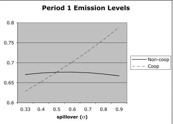
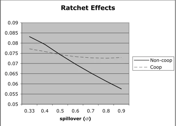
Simulation Result 4 The first period equilibrium emissions rate increases slowly for spillover levels between 0.33-0.6, and declines slowly for spillover levels greater than 0.6. The equilibrium ratchet effect, however, declines monotonically with σ, i.e., the higher the spillover, the smaller the noncoop-erative ratchet effect in equilibrium.
4.2
Cooperative R&D
Under cooperative R&D, the two-period problem consists of the same 6 steps as in Section 4.1, except at steps (2) and (5) where firms choose {xit, xjt}2
t=1 cooperatively, i.e., they maximize the sum of their (reduced-form) profits. We sketch the corresponding derivations in each step.
Steps 5 and 6. The calculation of second period output and research levels are as in Section 3.2, where the values of ¯xC
2 and ¯q2C are given by equation
(5) with k =kH or kL (depending on the firms’ type), and η = η2. Second
period profits are given by equation (4) with appropriate substitutions.
Step 4. As in the noncooperative R&D case, simulations indicate that low-cost firms will behave manipulatively in the first period. CARB maximizes the expected second-period social surplusEWC
2 (¯x C 2,Q¯
C
2, η2),where ¯QC2 = 2¯q C 2
and the expectation is taken with respect to the prior on k. The optimal emissions standard ¯ηC
2 equals
¯
ηC 2 =
aγ(2−kH −kL)A′
where A′ = 18γ−2(1 +σ)2
.
Steps 2 and 3. Firms choose their first period research levels cooperatively, followed by their noncooperative output levels. When firms are high-cost, ¯
xC
1,H and ¯q1C,H are given by (5) with k = kH and η = η1. When firms are
low-cost and manipulate, their first period research level is
˜
xC1,L= ¯x C 1,H −
(kH −kL) 4.5γη1
(1 +σ) (12)
whereas the output level ˜qC
1,L ≡q¯1C,H. Propositions analogous to Propositions
3 and 4 in the noncooperative case are easily derived here as well.
Step 1. CARB chooses an emissions standard η1 so as to maximize the
expected first-period social surplus EWC
1 (η1) given by
¯
ηC 1 =
aγB′
2µ−γF′ (13)
where
B′ = (1−kH)A′ (D′)2 +
(kH −kL)
D′ and
F′ = (1−kH)
2 A′ (D′)2 −
(kH −kL)2
(1 +σ)2 +
2(kH −kL)(1−kH)
D′ .
4.3
No pre-commitment R&D, profit levels and social
welfare
Comparing the ratchet effects as well as the first-period emission standards under the noncooperative and cooperative regimes, it is straightforward to derive that the cooperative emissions level is greater than the noncooperative one if and only if spillovers are large:
Proposition 5 Comparing the two R&D regimes,
(1) the cooperative emissions level η¯C
(2) the cooperative ratchet effect is also larger than the noncooperative one if and only if σ > 0.5.
Proposition 6 With high spillovers (σ > 0.5), the cooperative research lev-els in each period are higher than the noncooperative ones, i.e., x¯C
1,H >x¯N1,H,
¯
xC
2,H >x¯N2,H, x˜C1,L >x˜N1,L, and x¯2C,L >x¯N2,L.
Simulation Result 5 The first period equilibrium emissions rate under co-operative R&D is lower than under noncooperation for low spillover levels, and higher for high spillover levels. Similarly for the equilibrium ratchet effect under cooperative R&D as compared to the noncooperative ratchet effect.
The result above is apparent from Tables 1 and 2. From Table 3 follows this result:14
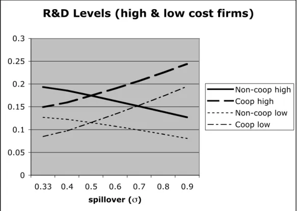
Simulation Result 6 For both high- and low-cost firms, the total coopera-tive research levels increase monotonically with spillover levels, while nonco-operative research levels decrease monotonically, regardless of whether firms are high- or low-cost.
Comparing total welfare and profit levels from the two periods (see Tables 4 and 5) yields the next result, an extension of the full-information Simulation Result 1 to this scenario with no pre-commitment.
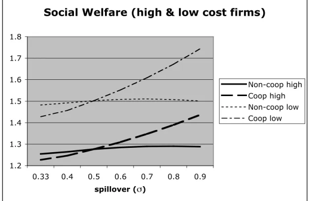
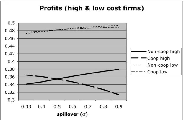
Simulation Result 7 For both high- and low-cost firms, the total social wel-fare levels are greater under noncooperative R&D for low spillover levels, and greater under cooperative R&D for high spillover levels. However, firm prof-its are higher under cooperation for low spillovers and under noncooperation for high spillovers.
14
An analogous result also holds in the original D’A&J paper (see p.1134): the non-cooperative R&D level x∗
Unlike in D’A&J, our simulation results show that for a high spillover rate, i.e., for σ > 0.5, firms’ profits are higher under non-cooperative R&D than under cooperative R&D, but social welfare is lower. The reverse is true for a low spillover rate, i.e., for σ <0.5. Hence, a conflict arises between the firms incentive to choose a cooperative R&D regime, and society’s interest.
5
Extensions
In this section, we consider two alternative scenarios, the first when CARB can precommit to an emissions standard for both periods, and the second a self-regulation scenario when firms choose the emissions standard coopera-tively.
5.1
Precommitment
Under the pre-commitment scenario, CARB sets an emission standard levelη
at the beginning of period 1, to be complied by both firms in both periods.15
As in the case of full information, there is no Bayesian updating of beliefs and, hence, the socially optimal solution to the two period problem is the solution to the one period problem repeated twice. The symmetric Nash equilibrium research and output levels under noncooperative R&D in both periods, ˆxN
and ˆqN, are given by equations (1) with appropriate substitutions forkandη.
CARB choosesthe emissions standard so as to maximize the expected social surplusEWN(ˆxN,QˆN, η), where ˆQN = 2ˆqN and the expectation is taken with
respect to the prior onk. Under the assumption thatkL andkH are equally likely, the value ˆηN for the emisisons standard under non-cooperative R&D is
identical to second period emissions standard without precommitment, i.e.,
15
ˆ
ηN = ¯ηN
2 from equation (7).
With cooperative R&D, the symmetric Nash equilibrium research and output levels under noncooperative R&D in both periods, ˆxC and ˆqC, are
given by equations (5) with appropriate substitutions for kand η. The emis-sions standard ˆηC is identical to the corresponding second period emissions
standard without precommitment, i.e., ˆηC = ¯ηC
2 from equation (11).
5.2
Self-regulation
Under self-regulation, firms set an emission standard cooperatively—in essence there is no CARB to audit firms costs and to set technology-forcing stan-dards, and firms choose an emission level that maximizes their joint profits. The emissions standard is assumed to be chosen once, before firms know their true type.16
When both firms do research noncooperatively after they have chosen the emission standard, the R&D investment ˙xN and output ˙qN decisions are
once again given by the equations in (1) with appropriate substitutions. Since the reduced-form profits of the firms are identical, maximizing joint profits is the same as maximizing any one firm’s profit function. Straightforward calculations yield:
˙
ηN = aγ(1−k)H 2µD2
−γ(1−k)2
H (14)
whereH = 9γ−2(2−σ)2
, andk ∈ {kL, kH}depending on whether firms are low-cost or high cost.
Similar calculations for the case where firms choose their research levels cooperatively yield ˙xC and output ˙qC as given by equations (5) and the
emissions standard by
˙
ηC = aγ(1−k)H ′ 2µ(D′)2
−γ(1−k)2
H′ (15)
16
where H′ = 9γ−2(2 +σ)2
.
6
Conclusions
The full-information scenario establishes a few benchmark results. First, low-cost firms do more research and produce a larger output than high-cost ones. At the same time, because a higher emissions standard is valued by society, CARB sets a higher standard when firms are low-cost and better able to meet that standard, resulting in lower profits. There is a fundamental conflict between firms’ private incentives to conduct cooperative R&D and society’s interests when consumers value vehicles with lower emissions: for high spillovers, firm profits are higher when they do not cooperate, while social welfare is higher if they do. Since the converse is true for low spillovers, firms have the incentive to engage in the opposite type of research to what is socially optimal.
When considering the asymmetric information scenario where CARB can-not credibly precommit to a single emission standard, low-cost firms always have the incentive to behave strategically and appear to CARB as if they are high-cost in attempting to keep the second period emission standard lower than what would otherwise be the case. This is achieved by lowering the research level undertaken, a ratchet effect that is larger under cooperation (noncooperation) for high (low) spillovers. As in the full-information case, social welfare is improved under cooperation for high spillovers, while firm profits are higher under noncooperation. This result indicates that the cur-rent permissive antitrust regulations that allow cooperative research efforts may not always be welfare improving — indeed, in our model, firms engage in cooperative R&D when spillovers are low and noncooperative research is socially optimal.
cost firms, simulations reveal that the emissions standard increases mono-tonically with the spillover level under cooperative R&D and the marginal impact of spillovers is more dramatic. But under noncooperative R&D, the marginal effect of spillovers is more muted and the level of research under-taken traces an inverted-U shape; thus high spillovers do not imply higher research levels in this case. The fact that emission levels decrease for high spillovers under noncooperation is at the heart of the conflict between firms’ incentives and social welfare.
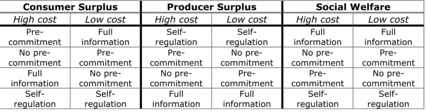
While we do not report on this extensively, we have considered two alter-native scenarios, one where CARB can precomit to an emission standard, and another where firms choose an emission standard themselves so as to maxi-mize joint profits. Comparing these four scenarios, simulations show (for the range of parameter values being considered) that social welfare is clearly (and unsurprisingly) maximized under full information, while producer surplus is minimized. Self-regulation on the other hand does the opposite: producer surplus is maximized while social welfare is minimized. Self-regulation is the worst scenario for consumers as emission standards are set too low. In be-tween, we obtain that when firms are high cost, social welfare is lower under pre-commitment than under no-commitment even with manipulation. On the other hand, when firms are low cost, pre-commitment yields a higher level of social welfare than no-commitment with manipulation (see Table 6 for details).
to introduce audting costs for CARB. Finally, we have only considered the possibility of both firms engaging in either cooperative and non-cooperative R&D simultaneously; in reality firms will could engage in private research in addition to cooperative research.
References
[1] D’Aspremont, C. and Jacquemin, A. (1988): “Cooperative and nonco-operative R&D in duopoly with spillovers.”American Economic Review, 78(5), pp. 1133-1137.
[2] Suzumura, K. (1992): “Cooperative and noncooperative R&D in an oligopoly with spillovers.”American Economic Review, 82(5), pp. 1307-1320.
Period 1 Emission Levels
0.6 0.65 0.7 0.75 0.8
0.33 0.4 0.5 0.6 0.7 0.8 0.9
spillover (s)
Non-coop Coop
Ratchet Effects
0.05 0.055 0.06 0.065 0.07 0.075 0.08 0.085 0.09
0.33 0.4 0.5 0.6 0.7 0.8 0.9
spillover (s)
Non-coop Coop
R&D Levels (high & low cost firms)
0 0.05 0.1 0.15 0.2 0.25 0.3
0.33 0.4 0.5 0.6 0.7 0.8 0.9
spillover (s)
Non-coop high Coop high Non-coop low Coop low
Social Welfare (high & low cost firms)
1.2 1.3 1.4 1.5 1.6 1.7 1.8
0.33 0.4 0.5 0.6 0.7 0.8 0.9
spillover (s)
Non-coop high Coop high Non-coop low Coop low
Profits (high & low cost firms)
0.3 0.32 0.34 0.36 0.38 0.4 0.42 0.44 0.46 0.48 0.5
0.33 0.4 0.5 0.6 0.7 0.8 0.9
spillover (s)
Non-coop high Coop high Non-coop low Coop low
Consumer Surplus Producer Surplus Social Welfare
High cost Low cost High cost Low cost High cost Low cost
Pre-commitment
Full information
Self-regulation
Self-regulation
Full information
Full information No
pre-commitment
Pre-commitment
Pre-commitment
No pre-commitment
No pre-commitment
Pre-commitment Full
information
No pre-commitment
No pre-commitment
Pre-commitment
Pre-commitment
No pre-commitment
Self-regulation
Self-regulation
Full information
Full information
Self-regulation
Self-regulation