FUZZY LOGIC AS A TOOL FOR UNCERTAINTY,
ROBUSTNESS AND RELIABILITY ANALYSES OF
MECHANICAL SYSTEMS
UNIVERSIDADE FEDERAL DE UBERLÂNDIA
FACULDADE DE ENGENHARIA MECÂNICA
ARINAN DE PIEMONTE DOURADO
FUZZY LOGIC AS A TOOL FOR UNCERTAINTY, ROBUSTNESS AND
RELIABILITY ANALYSES OF MECHANICAL SYSTEMS
Tese apresentada ao Programa de
Pós-graduação em Engenharia Mecânica da
Universidade Federal de Uberlândia, como parte
dos requisitos para a obtenção do título de
DOUTOR EM ENGENHARIA MECÂNICA.
Área de Concentração: Mecânica dos Sólidos e
Vibrações.
Orientador: Prof. Dr. Valder Steffen Jr.
Dados Internacionais de Catalogação na Publicação (CIP) Sistema de Bibliotecas da UFU, MG, Brasil.
D739f
2018 Dourado, Arinan de Piemonte, 1987- Fuzzy logic as a tool for uncertainty, robustness and reliability analyses of mechanical systems / Arinan de Piemonte Dourado. - 2018.
89 f. : il.
Orientador: Valder Steffen Junior.
Tese (Doutorado) - Universidade Federal de Uberlândia, Programa de Pós-Graduação em Engenharia Mecânica.
Disponível em: http://dx.doi.org/10.14393/ufu.te.2018.778 Inclui bibliografia.
1. Engenharia mecânica - Teses. 2. Lógica difusa - Teses. 3. Controle robusto - Teses. 4. Confiabilidade (Engenharia) - Teses. I. Steffen Junior, Valder. II. Universidade Federal de Uberlândia. Programa de Pós-Graduação em Engenharia Mecânica. III. Título.
I would like to express my sincere gratitude to my family, in special my mother for having provided to me the education basis that led me to all my accomplishments and for her encouragements to look for achievements that are more important.
I am grateful to have a true angel in my life, my wife Mirella, thank you for sharing my dreams and for helping me to make our dreams come true.
I thank also my colleges in the LMEst laboratory for the support you all assured to me during this journey, especially Prof. Dr. Aldemir Cavalini, whose contribution made this work possible. Thank you Prof. Dr. Leonardo Sanches for being a true friend along all these years.
I would also like to express my sincere thanks to my advisor Prof. Valder Steffen Jr, who I learned to admire not only professionally but also as a person. I will consider myself fulfilled if I can achieve half of your accomplishments.
A special thanks to the faculty and staff of FEMEC-UFU, and to my advisory committee members for their willingness on evaluating my thesis and contributing to its improvement.
Abstract
.
The main goal of this doctoral research work is to evaluate fuzzy logic as a tool for uncertainty, robustness and reliability analyses of mechanical systems. In this sense, fuzzy logic approaches are used on various design scenarios, such as the uncertainty analysis of rotating systems, robust balancing procedures, and reliability-based design problems. Firstly, the so-called α-level optimization technique is both numerical and experimentally evaluated in the context of uncertainty analysis of rotating systems. A numerical application considering a rotor test rig with uncertainties affecting shaft Young’s modulus and bearing stiffness is used to evaluate and compare fuzzy uncertainty analysis with well stablished stochastic procedures. Then, this fuzzy logic uncertainty analysis is used to predict the extreme responses of a flexible rotor supported by hydrodynamic bearings with uncertainties affecting oil properties. Afterwards, fuzzy logic is evaluated as a tool for robust optimization by means of two novel fuzzy logic balancing approaches: i) a non-parametric approach formulated to enhance the so-called IC method balancing robustness, and ii) a parametric methodology formulated to increase the balancing robustness of model-based balancing technique. In the first approach fuzzy logic tools, particularly fuzzy logic transformation and defuzzification procedures, are used to define a preprocessing stage in which system vibration responses sets are evaluated in order to obtain a more representative unbalance condition. In the second approach, fuzzy logic optimization is used to define fuzzy logic objective functions in which uncertainties affecting the balancing responses are assessed. Finally, a novel fuzzy logic reliability-based design methodology is proposed, revising the traditional fuzzy logic approach in terms of the reliability index. The resulting reliability design methodology consists of a nested algorithm in which an inner optimization loop is used to obtain the uncertain variables limits and an outer optimization loop evaluates a predefined fuzzy reliability index within the previously obtained bounds. Obtained results confirm fuzzy logic as a prominent tool for uncertainty, robustness and reliability analyses.
Resumo
O principal objetivo desta tese de doutorado é avaliar o uso da lógica nebulosa como uma ferramenta para análise de incerteza, robustez e confiabilidade de sistemas mecânicos. Neste sentido, abordagens baseadas em lógica nebulosa são definidas e utilizadas para a análise de incertezas em máquinas rotativas, a formulação de procedimentos de balanceamento robusto e para formulação de problemas de projetos baseados em confiabilidade. Primeiramente, a técnica conhecida como otimização de níves α é avaliada tanto numérica como experimentalmente para a análise de incertezas de máquinas rotativas. Uma aplicação numérica considerando um rotor com incertezas que influenciam o módulo de Young do eixo e as rigidezes dos mancais é usada para avaliar e comparar a análise de incertezas fuzzy com procedimentos estocásticos já estabelecidos. Então, este procedimento de lógica nebulosa é utilizado para prever as respostas extremas de um rotor flexível suportado por mancais hidrodinâmicos com incertezas que influem sobre as propriedades do lubrificante. Posteriormente a lógica nebulosa é avaliada como uma ferramenta para otimização robusta por meio de dois novos procedimentos de balanceamento robusto, a saber: i) uma abordagem não-paramétrica formulada para elevar a robustez do procedimento de balanceamento conhecido como método dos coeficientes de influência, e ii) uma abordagem paramétrica formulada para fazer aumentar a robustez do método de balanceamento baseado em modelos matemáticos representativos. Por fim, uma nova metodologia de lógica nebulosa para projetos baseados em confiabilidade é proposta, revisando a abordagem de lógica nebulosa tradicional em termos da métrica de confiabilidade. O procedimento proposto consiste de um algoritmo aninhado, no qual um laço interno é utilizado para obter os limites dos parâmetros incertos enquanto um laçoexterno avalia uma métrica de confiabilidade fuzzy predefinida, considerando os intervalos obtidos no laço interno. Resultados obtidos indicam a lógica nabulosa como uma ferramenta proeminente para análises de incerteza, robustez e confiabilidade.
_____________________________________________________________________
NOMENCLATURE
CHAPTER 2
SFEM Stochastic Finite Element Method
PCE Polynomial Chaos Expansion
FE Finite Element
MCS Monte Carlo Simulation
KL Karhunen-Lòeve
, one-dimensional random field in a Hilbert space
spatial component of a random field
random process
, autocovariance function
σ variance of a random field
ρ correlation coefficient
Ω a given geometry
eigenvalues of the autocovariance function
deterministic function
mean value of a random field
random variables
X classical set
x generic set elements
A subset
µA membership function
à fuzzy set
E Young’s modulus
ρ material density
υ Poisson’s coefficient
M mass matrix
Dg gyroscopic matrix
K stiffness matrix
Kst stiffness matrix resulting from the transient motion
W weight of the rotating parts
Fu unbalance forces
Fm shaft supporting forces
q generalized displacement
γ mass proportional damping coefficient
β stiffness proportional damping coefficient
kROT angular stiffness
FRF frequency response function
FRF FRFs generated by a FE model
FRF experimental FRFs
Ω operational rotation speed of the rotor
K(e) elementary stiffness matrix
KS(e) shaft elementary stiffness matrix
KB(e) bearings elementary stiffness matrix
shaft area moment of inertia
, correlation length
random elementary stiffness matrices
mean value of the bearings stiffness coefficients
dispersion level
SQP Sequential Quadratic Programming
RMS mean square convergence analysis
C bearings radial clearance
µh oil viscosity
Toil oil temperature
Outexp,i experimental vibration response
Outmodel,i FE model vibration response
CHAPTER 3
Up Rotor unbalance distribution
Vj Vibration amplitudes
αjp Influence coefficients
V0 Vibration responses for the original unbalance condition
U0 Original unbalance distribution
mt Trial weight
W1 Trial weight unbalance force
h Eccentricity
unb Unbalance condition fuzzy set
Npos Number of no rejections
Nneg Number of rejections
H0 Null hypothesis
α Significance level of a hypothesis test
p-value Statistic test metric
αmin Minimum significance level
αmax Maximum significance level
E Young’s modulus
ρ material density
υ Poisson’s coefficient
IDX Discs inertia moment in X direction
IDY Discs inertia moment in Y direction
IDZ Discs inertia moment in Z direction
kxx Self-alignment ball bearing stiffness coefficient in X direction
kzz Self-alignment ball bearing stiffness coefficient in Z direction
dxx Self-alignment ball bearing damping coefficient in X direction
dzz Self-alignment ball bearing damping coefficient in Z direction
F Model-based balancing objective function
Rotor original vibration responses in the model-based balancing
Pessimist objective function in robust model-based balancing Optimist objective function in robust model-based balancing and Upper and lower limits of uncertain parameters
∗, FE model vibration response with deterministic correction weights
and nominal configuration
, FE model vibration response at optimist configuration , FE model vibration response at pessimist configuration
CHAPTER 4
FLSFj Fuzzy limit state function
Rj Structural strength
Sj Structural stress
gj(x) Inequality constraints
x Vector of design variables
ηjαk Traditional reliability index
ηj′ Revised reliability index
fm Failure metric
xd Design variables
xr Random variables
xf Fuzzy variables
FUZZY LOGIC AS A TOOL FOR UNCERTAINTY, ROBUSTNESS AND
RELIABILITY ANALYSES OF MECHANICAL SYSTEMS
TABLE OF CONTENTS
CHAPTER 1: INTRODUCTION ... 3
CHAPTER 2: FUZZY UNCERTAINTY ANALYSIS ... 6
2.1. UNCERTAINTY ANALYSIS REVIEW ... 6
2.2. STOCHASTIC APPROACH... 7
2.2.1 MONTE CARLO SIMULATION ... 7
2.2.2 STOCHASTIC FINITE ELEMENT METHOD ... 8
2.3. FUZZY LOGIC ... 10
2.3.1 FUZZY VARIABLES ... 11
2.3.2 FUZZY DYNAMIC ANALYSIS ... 12
2.4. NUMERICAL VALIDATION ... 13
2.4.1 ROTOR TEST RIG ... 13
2.4.2 UNCERTAINTY SCENARIOS ... 16
2.4.3 FREQUENCY DOMAIN ANALYSIS ... 20
2.4.4 TIME DOMAIN ANALYSIS ... 23
2.5 EXPERIMENTAL VALIDATION ... 29
2.5.1 ROTOR TEST RIG ... 29
2.5.2 UNCERTAINTY ANALYSIS ... 34
CHAPTER 3: ROBUST OPTIMIZATION BY MEANS OF FUZZY LOGIC ... 42
3.1 ROTOR BALANCING REVIEW ... 42
3.2 NON‐PARAMETRIC EVALUATION ... 44
3.2.1 IC BALANCING METHOD ... 44
3.2.2 FUZZY LOGIC CONCEPTS ... 46
3.2.3 NUMERICAL APPLICATION ... 51
3.2.4 EXPERIMENTAL VALIDATION ... 56
3.3 PARAMETRIC EVALUATION ... 61
3.3.1 MODEL‐BASED BALANCING METHOD ... 61
3.3.2 ROBUST MODEL‐BASED BALANCING METHOD ... 63
3.3.3 NUMERICAL EVALUATION ... 65
4.1 RELIABILITY‐BASED OPTIMIZATION REVIEW ... 69
4.2 FUZZY SET THEORY REVISITED ... 71
4.3 TRADITIONAL FUZZY RELIABILITY ANALYSIS ... 72
4.4 PROPOSED FUZZY RELIABILITY ANALYSIS ... 74
4.5 NUMERICAL EVALUATION ... 76
4.5.1 NONLINEAR LIMIT STATE FUNCTION ... 76
4.5.2 CANTILEVER BEAM PROBLEM ... 77
4.5.3 CAR‐SIDE IMPACT PROBLEM ... 82
CHAPTER 5: FINAL REMARKS ... 86
REFERENCES ... 90
APPENDIX A: PUBLISHED AND SUBMITTED PAPERS ... 95
CHAPTER I
INTRODUCTION
The increasing demand for higher industrial productivity as driven the development of more efficient mechanical systems, implying on increasing reliability and robustness and lowering operational costs. Consequently, the development of more representative mathematical models is crucial in the context of modern engineering.
Mechanical systems in general are subjected to the effects of inherent uncertainties that arise mainly due to operational fluctuations, manufacturing errors, damage, wear or merely due to the lack of knowledge regarding the system itself. These effects can be directly related to system performance, durability and reliability and usually are unaccounted for in design stages.
Commonly, in the design or analysis of mechanical systems deterministic models are derived from known physical phenomena in an attempt to represent the system behavior. These deterministic models are unable to account for system uncertainties and usually an uncertainty analysis is performed in order to obtain the system extreme responses, which is essential for the assessment of system robustness and reliability.
In this sense, the main goal of this PhD thesis can be defined as the evaluation of fuzzy logic, a simpler mathematical representation of system uncertainties, aiming at uncertainty, robustness and reliability analyses. Uncertainty analysis can be viewed as a mathematical process that aims to obtain system extreme responses when exposed to the effect of uncertainties. Robustness can be interpreted as the system sensitivity with respect to the influence of uncertainties; consequently, robust system responses are as less sensitive as possible to system fluctuations. Reliability emphasizes on the achievement of predefined constraints related to design stability and/or safety performance. Figure 1.1 illustrates the concept of robustness and reliability.
intervals. Despite being relatively recent, fuzzy set theory is gaining more attention and successful applications have been reported in the literature (MÖLLER, GRAF and BEER, 2000; MÖLLER and BEER, 2004; OZBEN, HUSEYINOGLU and ARSLAN, 2014; DE ABREU
et al., 2015).
a) robustness b) reliability
Figure 1.1 Concept of robustness and reliability.
In the context of the research effort at the LMEst laboratory (UFU – Federal University of Uberlândia) on uncertainty analysis and robustness evaluation, the present contribution is a continuation of the following research projects as developed by:
BUTKEWITSCH (2002): evaluated a robust optimization of safety vehicular components;
KOROISHI et al. (2012): considered uncertainties effects on a flexible rotor by means of the Stochastic Finite Element Method (SFEM);
LARA-MOLINA, KOROISHI and STEFFEN Jr (2015): evaluated uncertainty effectes on a flexible rotor considering fuzzy and random-fuzzy parameters;
CAVALINI Jr et al. (2015): proposed a fuzzy approach to assess uncertainties effects in a flexible rotor supported by fluid film bearings;
CARVALHO (2017): adopted a model based balancing appraoch to obtain robust balancing responses considering uncertainties through Monte Carlo simulations.
Consequently, the present contribution aims to evaluate the fuzzy logic approach as tool for uncertainty, robustness and reliability analyses. In this sense, a fuzzy uncertainty analysis methodology is evaluated both numerically and experimentally for a flexible rotor, wherein the proposed methodology performance is compared with well-established uncertainty
Robust Optimum
Global Optimum
∆
∆
∆
∆
x2
x1 Feasible Region
Deterministic Optimum Reliable
Optimum
analysis techniques. In the sequence, two distinct approaches based on fuzzy set theory and fuzzy uncertainty analysis are proposed and evaluated for the robust balancing of rotating machines. Finally, a fuzzy reliability-based design methodology is formulated and evaluated for the reliability-based design of mechanical systems.
The outline of the remainder of this contribution is as follows:
Chapter 2: Presents the proposed fuzzy uncertainty analysis methodology and the results of the numerical and experimental validation of the proposed approach. A brief discussion of the obtained results is also addressed.
Chapter 3: Introduces the proposed fuzzy robust balancing approaches. Both methodologies are presented; numerical and experimental results are obtained and discussed.
Chapter 4: Focuses on the proposed fuzzy reliability-based design approach, addressing its formulation and numerical results obtained.
CHAPTER II
FUZZY UNCERTAINTY ANALYSIS
In this chapter, the so-called α-level optimization procedure for fuzzy uncertainty analysis is presented and discussed. First, the performance of the proposed methodology is numerically compared with well-established uncertainty analysis approaches, whereas the dynamic responses of a horizontal rotor test rig are evaluated under the influence of uncertain rotor shaft Young’s modulus and uncertain bearing stiffness. Then, the proposed fuzzy uncertainty analysis methodology is experimentally validated for a flexible rotor containing three rigid discs and supported by two cylindrical fluid film bearings.
The chapter begins by addressing the key issues related to uncertainty analysis and the proposed fuzzy approach. After, the numerical validation of the proposed methodology is presented. Then, the experimental validation of the fuzzy approach is demonstrated. Finally, a brief discussion of the obtained results is presented
.
2.1. Uncertainty Analysis Review
There are different techniques that can be used to modeling uncertainties in mechanical systems. The stochastic approach exhibits a longer history of applications on mechanical systems, while the fuzzy logic technique is recently gaining more attention.
The stochastic methodology is based on the probability theory. GHANEM and SPANOS (1991) contextualize the stochastic approach within the scope of structural dynamics through the Stochastic Finite Element Method (SFEM) and the so-called Polynomial Chaos Expansion (PCE) technique. The fuzzy logic approach is an intuitive technique based both on fuzzy sets and on the possibility theory. KOSKO (1990) brings a review about the main issues on fuzziness and probability.
Concerning rotor dynamics associated problems, RÉMOND, FAVERJON and SINOU (2011) assessed the flexible rotor dynamics subject to uncertain parameters by SFEM and
the Karhunen-Lòeve series expansion (KL series expansion). SEGUÍ, FAVERJON and JACQUET-RICHARDET (2013) investigated the effects of uncertainties affecting the material properties of blades in a multistage bladed disc system by using the PCE technique. More recent rotor dynamic applications of the stochastic approach can be found in (SEPAHVAND, NABIH and MARBURG, 2015; SINOU and JACQUELIN, 2015; SINOU, DIDIER and FAVERJON, 2015).
Following the fuzzy approach, RAO and QIU (2011) presented a methodology for the fuzzy analyses of nonlinear rotor-bearing systems along with numerical results that were presented to demonstrate the computational feasibility of the proposed approach. LARA-MOLINA, KOROISHI and STEFFEN JR. (2015) analyzed the dynamics of flexible rotors under uncertain parameters modeled as fuzzy and fuzzy random variables. CAVALINI JR et al. (2015) evaluated the dynamic behavior of a flexible rotor with three rigid discs, supported by two fluid film bearings. The uncertainties were considered as affecting the oil viscosity and the radial clearance of both bearings that support the machine.
Both the stochastic and fuzzy logic approaches were applied to the analysis of uncertainties affecting the steady state characteristics and the overall dynamic behavior of rotating machines. In this chapter, a systematic study dedicated to compare both methodologies is presented aiming to assess their suitability regarding rotor dynamics applications.
2.2. Stochastic Approach
In the stochastic approach, the purpose is to evaluate the randomness and the variability of the uncertain parameters of the model. Thereby, the uncertainties are modeled either as random variables or as random fields. Among the various stochastic techniques that aim at accomplishing this goal, the SFEM and the Monte Carlo Simulation (MCS; i.e., as stochastic solver) are extensively used (KUNDU et al., 2014; JENSEN and PAPADIMITRIOU, 2015; SEPAHVAND, 2016).
2.2.1 Monte Carlo Simulation
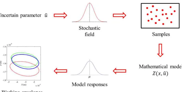
model of the analyzed mechanical system, generating the uncertain quantity response (which implies a high computational cost). Therefore, the statistical characteristics of the outputs (i.e., the model responses) can be estimated and the variability of the model can be inferred. Figure 2.1 presents a schematic representation of the main features associated with MCS. More details concerning this approach can be found in (BINDER, 1979; NEWMAN and BARKEMA, 2001).
Figure 2.1 - Schematic representation of the main features associated with MCS.
It is worth mentioning that the convergence of the MCS is practically guaranteed in different applications, making this stochastic solver extensively used for the cases in which the statistical characteristic of the mechanical system is not available (HUDSON and TILLEY, 2014; BAO and WANG, 2015; CHEN and SCHUH, 2015; CADINI and GIOLETTA, 2016).
2.2.2 Stochastic Finite Element Method
If the parameters of the mechanical system are uncertain (modeled as random fields), the model should be represented by stochastic differential equations. Adopting the same spatial discretization used in the classical FE method, an incomplete representation of the random field is obtained. Therefore, a series expansion technique is used to discretize the random dimension efficiently. In this sense, the KL series expansion (GHANEM and SPANOS, 1991) or various orthogonal series (ZHANG and ELLINGWOOD, 1994) can be applied.
The KL series expansion is based on the application of the spectral theorem for compact normal operators in conjunction with Mercer’s theorem, which connects the spectral representation of a Hilbert-Schmidt integral operator to the corresponding Hilbert-Schmidt kernel. LOÈVE (1977) and GHANEM and SPANOS (1991) provide an interesting discussion of the mathematical basis involving KL series expansion. The key aspects of KL series expansion related to uncertainty analysis are presented next.
The KL series expansion of a random field is based on the spectral decomposition of its auto covariance function. It is a continuous representation of the random field expressed by the superposition of orthogonal random variables, which are weighted by deterministic spatial functions (GHANEM and SPANOS, 1991).
The auto covariance function of a one-dimensional random field , , where denotes the spatial dependence of the field and represents a random process, can be defined as shown in Eq. (2.1).
, , (2.1)
in which σ denotes the variance of the field and ρ is the correlation coefficient.
The set of deterministic functions for which any event of the field is expanded with respect to a given geometry Ω is defined by the eigenvalue problem presented in Eq. (2.2).
∀ 1, … , Ω (2.2)
where are the eigenvalues of the auto covariance function , and is a deterministic function.
, (2.3)
where is the mean value of the field, are the eigenvalues of the auto covariance function , , and are random variables.
The intrinsic eigenvalue problem associated with the series expansion can be analytically solved only for a few auto covariance functions and geometries. Detailed solutions for triangular and exponential covariance functions and one-dimensional homogeneous random fields are shown in GHANEM and SPANOS (1991) for Ω , . The eigenvalue problem has to be solved numerically regarding different cases.
In the KL series expansion of a Gaussian process, the random variables are independent standard normal random variables. This property is useful in practical applications, especially for the SFEM. Moreover, the convergence of the series representation given by Eq. (2.3) is guaranteed in the cases for which a Gaussian process is considered (LOÈVE, 1977).
Both series expansions procedures (i.e., KL and orthogonal series) aim at determining the random variables that are related to the stochastic differential equations that represent the mechanical system. The KL and orthogonal series decompositions are not able to solve these equations. In order to obtain the solution of the differential equations, a stochastic solver is used (e.g., MCS). The solver should infer the variability of the system through the evaluation of the random variables.
2.3. Fuzzy Logic
ZADEH (1965) first introduced the fuzzy logic theory with the purpose of formalizing the notion of graded membership, as represented by the so-called membership function. The fuzzy sets are understood as the counterpart of the Boolean notion of regular sets, in a sense that in a fuzzy set an element can belong, not belong, or partially belong to the set.
element x of the set. The notion of degree of uncertainty is the base of the possibility theory (ZADEH, 1968) and the main tool for fuzzy uncertainty analysis.
Based on the concept of degree of uncertainty and through the fuzzy set theory, uncertainties can be modeled as fuzzy variables for the cases in which the statistical process that describes the random variables is unknown. The uncertain parameters are modeled as fuzzy numbers, where the actual value of the parameter is unknown, but limited to an interval weighted by a membership function. At this point, it is important to highlight that the membership function is a possibility distribution, not a probability distribution as required in the stochastic theory. Possibility is the measure of whether an event can happen, while probability is a measure of whether an event will happen. Therefore, the possibility distribution of a given uncertain parameter u quantifies the possible values that this parameter can assume. A probability distribution quantifies the chances that the uncertain parameter u has to assume a certain value x.
2.3.1 Fuzzy Variables
Let X be a universal classical set of objects whose generic elements are denoted by x. The subset A (A ∈ X) is defined by the classical membership function µA: X → {0,1}, shown in Figure 2.2, in which à represents the fuzzy set and xl and xr are the lower and upper bounds of the fuzzy set support, respectively. Furthermore, a fuzzy set is defined by means of the membership function µA: X → [0,1], being [0,1] a continuous interval. The membership function indicates the degree of compatibility between the element x and the fuzzy set . The closer the value of µA(x) is to 1, more x belongs to .
A fuzzy set is completely defined by (where 0 ≤ µA ≤ 1):
, ( )
AA
x
x
x
X
(2.4)a) Fuzzy set. b) The α-levels.
The fuzzy set can be represented by means of subsets that are denominated α-levels (see Figure 2.2), which correspond to real and continuous intervals.
2.3.2 Fuzzy Dynamic Analysis
The fuzzy dynamic analysis is an appropriate method to map a fuzzy vector of parameters onto output fuzzy functions by using the deterministic model of the mechanical system. In structural analysis, the combination of uncertainties modeled as fuzzy variables with the deterministic model based on the finite element method is denominated fuzzy finite element method. The fuzzy dynamic analysis includes two stages, based on the α-level optimization (MÖLLER, GRAF and BEER, 2000), as shown in Figure 2.3. In the first stage, for computational purposes, the input vector that corresponds to the fuzzy parameter is discretized by means of the α-level representation (see Figure 2.2). Thus, each element of the fuzzy parameter vector is considered as an interval. The second stage is related to solving an optimization problem. This optimization problem consists in finding the maximum or minimum value of the output at each α-level.
The fuzzy analysis of a transient time-domain system demands the solution of a large number of optimization problems regarding all α-levels of interest for each considered time step. Each upper and lower bounds of the system analysis at a given time instant is obtained from an optimization algorithm (VANDERPLAATS, 2007). The output value of the transient analysis at the evaluated time-step constitutes the objective function. The inputs to this function are the uncertain parameters described previously as fuzzy, or fuzzy random variables.
The fuzzy dynamic analysis based on the α-level optimization method is an eficient methodology for uncentainty analysis. However, the effectiveness of the method is highlly related to the performance of the optimization technique.
Figure 2.3 - The α-Level optimization
2.4. Numerical Validation
The numerical analysis considered the influence of uncertainties in the Young’s modulus of the shaft of a rotor test rig and in the stiffness of the bearings of the rotating machine, on the dynamic response of the system. A straightforward numerical method was applied to simulate the dynamic responses of a representative Finite Element model (FE model) of the flexible rotor with two rigid discs and two self-alignment ball bearings. It is worth mentioning that the FE model was derived by using the approach previously presented by (CAVALINI JR et al., 2016).
2.4.1 Rotor Test Rig
Figure 2.4a shows the rotor test rig used as a reference in the numerical validation process of the proposed fuzzy uncertainty analysis, which was mathematically represented by a model with 33 finite elements (FE model; Figure 2.4b).
a) Test rig b) FE model
Figure 2.4 - Experimental test rig (a) and its corresponding FE model (b)
Equation 2.5 presents the equation of motion that governs the dynamic behavior of the flexible rotor supported by roller bearings (LALANNE and FERRARIS, 1998).
Ω Ω (2.5)
where M is the mass matrix, D is the damping matrix, Dg is the gyroscopic matrix, K is the stiffness matrix, and Kst is the stiffness matrix resulting from the transient motion. All these matrices are related to the rotating parts of the system, such as couplings, discs, and shaft. W
stands for the weight of the rotating parts, Fu represents the unbalance forces, Fm is the vector of the shaft supporting forces produced by the ball bearings (incorporated as stiffness and damping coefficients in the matrix K), and q is the vector of generalized displacement.
Due to the size of the matrices involved in the equation of motion, the pseudo-modal method is used to reduce the dimension of the FE model and provided the solution, as proposed by LALANNE and FERRARIS (1998). In this work, the first twelve vibration modes of the rotor were used to generate the displacement responses.
directions X - horizontal and Z - vertical of the node #1). Further information regarding the model updating procedure adopted in this work can be found in CAVALINI JR et al. (2016).
The entire frequency domain process (i.e., comparison between simulated and experimental frequency response functions; FRF) was performed 10 times, considering 100 individuals in the initial population of the optimizer. The objective function adopted is presented in Eq. (2.6). For this case only the regions close to the peaks associated with the natural frequencies were taken into account.
FRF FRF
FRF
(2.6)
where n is the number of FRFs used in the minimization procedure, FRF is the FRFs generated by the FE model, is the vector containing the proposed unknown parameters, and FRF is the experimental FRFs measured on the test rig.
The experimental FRF were measured for the test rig at rest by applying impact forces along the X and Z directions of both discs, separately. The response signals were measured by two proximity probes positioned along the same directions of the impact forces, resulting 8 FRFs. The measurements were performed by the analyzer Agilent® (model 35670A) in a range of 0 to 200 Hz and a frequency resolution of 0.25 Hz.
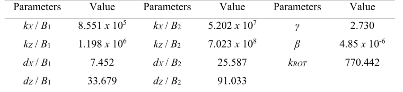
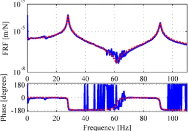
Table 2.1 summarizes the parameters determined in the end of the minimization process associated with the smallest fitness value (i.e., value of the objective function; Eq (6)). Figure 2.5 compares simulated and experimental FRFs, and the associated phase diagram, considering the parameters shown in Table 2.1. Note that the FRF generated from the FE model is satisfactorily close to the one obtained directly from the test rig.
Table 2.1 Parameters determined by the model updating procedure
Parameters
Value
Parameters
Value
Parameters
Value
k
X/
B
18.551
x
10
5k
X/
B
25.202
x
10
7γ
2.730
k
Z/
B
11.198
x
10
6k
Z/
B
27.023
x
10
8β
4.85
x
10
-6d
X/
B
17.452
d
X/
B
225.587
k
ROT770.442
d
Z/
B
133.679
d
Z/
B
291.033
*
k
: stiffness [N/m];
d
: damping [Ns/m]
.
updated FE model. The operational rotation speed of the rotor Ω was fixed to 1200 rev/min and an unbalance of 487.5 g.mm / 00 applied to the disc D1 was considered. Note that the responses are close, as for the FRF previously shown, thus validating the updating procedure performed.
Figure 2.5 Simulated (
‐ ‐ ‐
) and experimental (──
) FRFs, and associated phases, obtained from impact forces on D1 (X direction and S8X).Figure 2.6 Simulated (
──
) and experimental (──
) orbits for the rotor under consideration.2.4.2 Uncertainty Scenarios
values. It is worth mentioning that even these small variations can affect the dynamic behavior of the rotor system, influencing its performance, life, and reliability. The second uncertain scenario is dedicated to the analysis of the orbits and unbalance responses (run-up tests) of the rotor, introducing variations on the stiffness coefficients kX and kZ of the bearing B1 (see Figure 2.4 and Table 2.1).
Three different methodologies were used to model the uncertain parameters of the rotating system (i.e., the Young’s modulus and the stiffness coefficients). Regarding the stochastic theory, two different methodologies were tested. In the first approach, the variability of the system was estimated through MCS associated with the Latin Hypercube sampling technique (see VIANA et al., 2007). No discretization procedure was used to discretize the random variables of the system; the deterministic FE model was used to evaluate the generated samples. From now on, this methodology will be referred to as MCS approach along the text, in a direct reference to the stochastic solver used to infer the variability of the system. The second approach is based on the SFEM associated with KL series expansion, considering an exponential autocovariance function. In this case, the random variables are discretized through a series expansion technique and evaluated by using the SFEM model. MCS combined with Latin Hypercube is used to solve the associated stochastic problem. This methodology will be referred to as KL method.
Note that the main diference between the two stochastic methodologies is associated with the discretization of the random variables. No discretization is considered in the first approach (i.e., MCS approach); while for the second methodology (i.e., KL method), a random discretization is performed to completely represent the random variables.
It is important to point out that the uncertain parameters were modeled as Gaussian random fields in both approaches. Gaussian random fields were adopted since it is expected that the realizations of the considered uncertain parameters are concentrated and symmetrically dispersed around their nominal values, approximately thus a 3σ model of Gaussian fields. Besides, another interesting feature of Gaussian fields is its guarantee convergence in the KL series expansion (LOÈVE, 1977), as previously mentioned. Also, in this contribution the interest in the uncertainty analysis is in the rotor working envelopes, so if other random fields, for instance, uniform fields, were selected, if the dispersion (3σ) were the same, is expected that obtained results to be identical, since the extreme realizations of the random field were note altered.
associated with K in Eq. (2.5)). Only the stiffness matrix of the rotating machine was parametrized, since the considered uncertain parameters are associated only to K.
(2.7a) (2.7b)
, (2.7c)
where KS(e) is the elementary stiffness matrix of the shaft (following the Timoshenko beam theory), and KB(e) is the elementary stiffness matrix associated with the bearings. In this formulation the shaft and bearings stiffness are considered to be in series resulting in the resulting elementary matrix . Also, represent the area moment of inertia of the shaft and E is the Young’s modulus of the shaft. Further, KB(e) is considered to be a function of and . The parameters and designate the stiffness coefficients of the bearings along the X and Z directions, respectively (see the deterministic parameters in Table 2.1).
As presented in Eq. (2.3), the KL series decomposition of a random field requires the knowledge of the eigenvalues and eigenfunctions of the random field associated with the autocovariance function. Considering a one-dimensional Gaussian field, GHANEM and SPANOS (1991) have shown that the eigen problem associated with the exponential covariance function presented in Eq. (2.8) has an analytical solution in the domain Ω
, .
, | |/ , (2.8)
where , ∈ 0, and , indicates the correlation length, characterizing the decreasing behavior of the covariance with respect to the distance between the observation points along the y direction.
Considering the property of the covariance function, the eigenvalues and eigenfunctions are given as a function of the roots 1 of two transcendental equations through a procedure that can be summarized as follows:
For r odd, with r 1:
,
, , ,
where 1⁄ ⁄2 ⁄2 and is the solution of the transcendental equation presented in Eq. (2.10).
1 , tan 0 (2.10)
defined in the domain 1 , .
For r even, with r 1:
,
, , ,
(2.11)
where 1⁄ ⁄2 ⁄2 and is the solution of the transcendental equation presented in Eq. (2.12).
, tan 0 (2.12)
defined in the domain , .
From the solution of the eigenproblem shown previously, the elementary random matrices of the shaft can be computed by using Eq. (2.13).
(2.13)
where is the random process and the random matrices are calculated by using Eq. (2.14).
(2.14)
where is the matrix of material properties in which the parameters and were factored-out.
The elementary matrices of the bearings are obtained by applying a dyadic structural transformation rather than an integration scheme as in the case of the shaft. The corresponding
uncertainties are introduced by using , where designates the mean
Further information regarding the parametrization procedure can be found in KOROISHI et al. (2012).
From the stochastic finite element matrices and by performing the standard FE matrix assembling procedure, the frequency domain and the time domain responses of the rotating machine can be obtained. The stochastic model of the flexible rotor has to be solved by a stochastic solver. As mentioned, in this contribution the stochastic model was solved through MCS combined with the Latin Hypercube technique.
Finally, the third methodology used to model the uncertain parameters of the rotating system (i.e., the Young’s modulus and the stiffness coefficients) is based on the fuzzy logic approach. In this case, the uncertain parameters are modeled as fuzzy triangular numbers (i.e., fuzzy variables) and mapped through the α-level optimization method. The Sequential Quadratic Programming algorithm (SQP; see (VANDERPLAATS, 2007)) was used to perform the required minimizations and maximizations (see Figure 2.3). The respective optimization problems are monomodal, thus allowing the direct optimization procedure to find global optimal solutions.
2.4.3 Frequency Domain Analysis
This analysis is confined to the frequency domain, as being characterized by the envelopes of the FRFs of the rotor responses. In this case, the influences of the uncertainties affecting the Young’s modulus of the shaft on the dynamic behavior of the system are evaluated.
Regarding the stochastic procedures (i.e., MCS approach and KL method), the inherent uncertainty was modeled as a Gaussian random field with nominal value E = 205 GPa with a deviation of ±5% (3 model, i.e. E±15%). The convergence of the response variability was verified regarding the number of terms retained in the truncated KL expansion series (nKL) and the number of samples used for MCS (nS). In order to determine nKL and nS, the mean square convergence analysis (RMS) with respect to the independent realizations of the FRF was obtained according to Eq. (2.15).
∑ | | (2.15)
Figure 2.7 presents the convergence analysis performed for the MCS approach and for the KL method (Figure 2.7a and Figure 2.7b, respectively). The number of terms retained in the series was verified, in which the convergence was achieved for 250 and 40.
a) nS b) nKL
Figure 2.7 Convergence verification for the frequency domain analysis.
Regarding the fuzzy approach, the uncertain parameter was modeled as a fuzzy triangular number with the same nominal value and deviation adopted for the stochastic procedures (i.e., 205 15% GPa). For the fuzzy uncertainty analysis, the objective function related to the α-level optimization procedure was the norm of the vector; i.e., the lower bound corresponds to the value that minimizes the system response and the upper bound is related to the value that maximizes the system response.
The uncertainty analysis in the context of rotating machines can be performed aiming at different goals. In the case of both robust design and robust control design, the objective of uncertainty analysis is to obtain the minimum and maximum responses of the rotor (i.e., the working envelopes). In the present contribution, the fuzzy logic approach was confined to the uncertainty level 0 of the model. Clearly, the stochastic analysis was formulated to obtain the minimum and maximum responses of the rotating machine.
Figure 2.8 shows the comparison between the uncertain envelopes of the rotor FRFs obtained by the stochastic and fuzzy methodologies. In this case, the FRFs were obtained by considering the force applied along the X direction of the disc D1 and the measures obtained from the sensor S8X (see Figure 2.5). Note that the results obtained by the different approaches are similar. Table 2.2 summarizes the results shown in Figure 2.8, in which the
M
ean Squar
e V
alue
number of terms
0 5 10 15 20 25 30 35 40 45 50
M
ean Squar
e V
alue
10-3
0 0.5 1 1.5 2 2.5 3 3.5 4 4.5
referred upper and lower limits (and the related values of Young’s Modulus) indicates the FRFs (H) working envelopes bounds.
a) MCS versus Fuzzy b) MSC versus KL
c) Fuzzy versus KL d) MCS, KL, and Fuzzy
Figure 2.8 FRFs determined for different methods of uncertainty analysis (…. deterministic FRF; see Figure 2.5).
Table 2.2 Results for the frequency domain analysis.
Method Lower Limit Upper Limit
(GPa)* (GPa)**
MCS 235.52 6.4 x 10⁻⁴ 174.31 7.04 x 10⁻⁴
KL 235.63 6.4 x 10⁻⁴ 174.37 7.06 x 10⁻⁴
Fuzzy 235.75 6.4 x 10⁻⁴ 174.25 7.04 x 10⁻⁴
* indicates the Young’s modulus value that generates the minimum response. ** represents the Young’s modulus value that generates the maximum response.
0 10 20 30 40 50 60 70 80 90 100
Frequency[Hz]
10-8 10-7
10-6
10-5
10-4
10-3
Monte Carlo Fuzzy
0 10 20 30 40 50 60 70 80 90 100
Frequency[Hz]
10-8
10-7
10-6
10-5 10-4 10-3
Regarding the associated computational cost, the fuzzy logic approach required 14 evaluations of the FE model, while the stochastic methods required 250 evaluations of the deterministic model (number of samples).
2.4.4 Time Domain Analysis
The time domain analyses (i.e., rotor orbits and run-up test) were performed considering the uncertainties affecting the stiffness coefficients kX and kZ of the bearing B1 (see Table 2.2). For the stochastic methods, the uncertain parameters were modeled as Gaussian random fields with nominal values of kX = 8.551x10⁵ N/m and kZ = 1.198x10⁶ N/m (see Table 2.1) with a deviation of ±10% (3 model).
Regarding the rotor orbits, the operational rotation speed of the rotor Ω was fixed to 1200 rev/min and an unbalance of 487.5 g.mm / 00 was applied to the disc D1 (see Figure 2.6). A simulation time of 10 seconds with steps of 0.001 seconds was adopted.
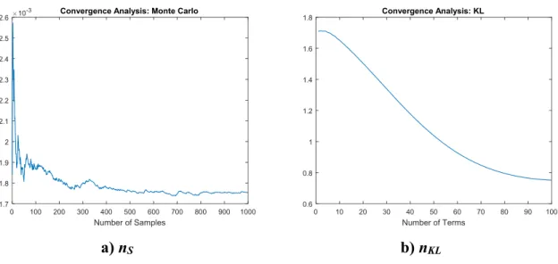
The convergence of the response variability was also verified in terms of the number of samples nS for the MCS approach and the number of terms nKL in the KL expansion. Analogous to the frequency domain analysis, the RMS value with respect to the independent realizations of the orbits was performed - Eq. (15) - considering that represents the orbits computed by the deterministic model and represents the orbits computed for the realization . Figure 2.9 presents the convergence analysis performed for both the MCS approach and KL method (Figure 2.9a and Figure 2.9b, respectively). Convergence was achieved for 500 and 100.
a)
n
Sb)
n
KLFigure 2.9 Convergence verification for the time domain analysis associated with the orbits of the rotor.
Number of Samples
0 100 200 300 400 500 600 700 800 900 1000 10-4
1.5 2 2.5 3 3.5 4
4.5 Convergence Analysis: Monte Carlo
Number of Terms
0 10 20 30 40 50 60 70 80 90 100 10-5
3 4 5 6 7 8 9 10 11
Regarding the fuzzy approach, the uncertain parameter was modeled as belonging to a fuzzy triangular function with the same nominal value and deviation adopted for the stochastic procedures (i.e., kX = 8.551x10⁵ N/m and kZ = 1.198x10⁶ N/m with a deviation of ±30%).The objective function related to the α-level optimization procedure was the norm of the displacement vector.
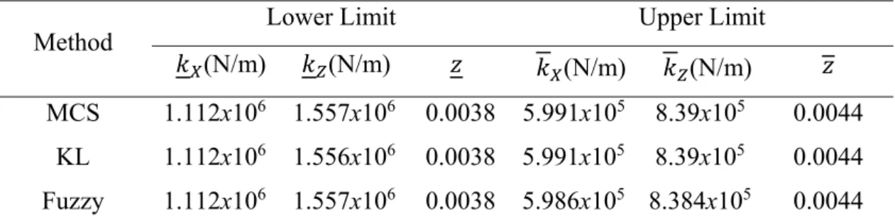
Figure 2.10 shows the comparison between the uncertain envelopes of the rotor orbits obtained by using the stochastic and fuzzy methodologies. Note that the results determined by these two approaches are similar. However, MCS approach leads to a bigger stiffness coefficient kZ. Therefore, small vibration amplitudes can be observed along the Z direction as compared with the results obtained by the KL method and the fuzzy approach. Table 2.3 summarizes the results shown in Figure 2.10 in which the referred upper and lower limits (and the related values of stiffness coefficients) indicates working envelopes bounds of the of the orbits (z). The fuzzy logic approach required 26 evaluations of the FE model and the stochastic methods required 500 evaluations of the deterministic model.
Regarding the run-up test, the operational rotation speed Ω of the rotor was considered as varying linearly from 0 to 3000 rev/min (simulation time of 10 seconds; steps of 0.001 seconds). An unbalance of 487.5 g.mm / 00 was applied to the disc D1.
The convergence of the response variability was also verified in terms of the number of samples nS for the MCS approach and the number of terms nKL for the KL expansion (see Figure 2.11). Similarly, to the analyses performed for the rotor orbits, the convergence of the RMS value was obtained for 500 and 100.
Figure 2.12 presents the comparison between the envelopes of the rotor responses (run-up test from 0 to 3000 rev/min in 10 seconds) determined along the X direction of the disc D1. Note that the amplitudes associated with the lower limit were similar to the ones obtained by using the fuzzy and MCS approaches. A similar behavior could not be verified by using the KL method. However, different values of amplitudes were observed in all of the remaining unbalance responses. Table 2.4 summarizes the results shown in Figure 2.12.
Similar to the orbits analysis, in the run-up test the fuzzy logic approach required 26 evaluations of the FE model while the stochastic methods required 500 evaluations of the deterministic model.
a) MCS versus Fuzzy b) MSC versus KL
c) Fuzzy versus KL d) MCS, KL, and Fuzzy
Figure 2.10 Orbits determined for the different uncertainty methods (-.-.- deterministic response; see Figure 2.6).
Table 2.3 Results for the time domain analysis associated with the rotor orbits.
Method
Lower Limit
Upper Limit
(N/m)
(N/m)
(N/m)
(N/m)
MCS
1.112
x
10
61.557
x
10
60.0038 5.991
x
10
58.39
x
10
50.0044
KL
1.112
x
10
61.556
x
10
60.0038 5.991
x
10
58.39
x
10
50.0044
Fuzzy
1.112
x
10
61.557
x
10
60.0038 5.986
x
10
58.384
x
10
50.0044
* indicates the stiffness coefficients that generates the minimum response . ** represents the stiffness coefficients that generates the maximum response .
-6 -4 -2 0 2 4 6
Horizontal (m) 10-5
-5 -4 -3 -2 -1 0 1 2 3 4 5 10-5
KL MC
-6 -4 -2 0 2 4 6
Horizontal (m) 10-5
-5 -4 -3 -2 -1 0 1 2 3 4 5 10-5
MC Fuzzy
-6 -4 -2 0 2 4 6
Horizontal (m) 10-5
-5 -4 -3 -2 -1 0 1 2 3 4 5 10-5
KL Fuzzy
-6 -4 -2 0 2 4 6
Horizontal (m) 10-5
-5 -4 -3 -2 -1 0 1 2 3 4 5 10-5
a)
n
Sb)
n
KLFigure 2.11 Convergence verification for the time domain analysis associated with the linear run-up test.
Table 2.4 Results for the time domain analysis associated with the run-up test.
Method
Lower Limit
Upper Limit
(N/m)
(N/m)
(N/m)
(N/m)
MCS
1.109
x
10
61.101
x
10
60.0291 5.987
x
10
59.968
x
10
50.0351
KL
1.089
x
10
61.063
x
10
60.0293 6.104
x
10
51.526
x
10
60.0347
Fuzzy
1.091
x
10
61.083
x
10
60.0291 6.596
x
10
51.196
x
10
60.0349
* indicates the stiffness coefficients that generates the minimum response . ** represents the stiffness coefficients that generates the maximum response .
Through numerical simulations, the stochastic and fuzzy approaches were compared in terms of uncertain envelopes generated by the analysis of the dynamic behavior of a flexible rotor. For this aim, uncertainties were introduced in the Young’s modulus of the shaft and the stiffness coefficients of the bearing.
The evaluated methodologies presented similar results regarding the FRFs of the rotating machine, suggesting that the proposed methods lead to equivalent results. However, this equivalence was not verified in the time domain analysis.
Number of Samples
0 100 200 300 400 500 600 700 800 900 1000 10-3
1.7 1.8 1.9 2 2.1 2.2 2.3 2.4 2.5
2.6 Convergence Analysis: Monte Carlo
Number of Terms
0 10 20 30 40 50 60 70 80 90 100 0.6
0.8 1 1.2 1.4 1.6
a) Upper limit – MCS versus Fuzzy b) Lower limit – MCS versus Fuzzy
c) Upper limit – MSC versus KL d) Lower limit – MSC versus KL
e) Upper limit – Fuzzy versus KL f) Lower limit – Fuzzy versus KL
Figure 2.12 Run-up responses determined for the different uncertainty approaches.
Speed (rev/min)
1400 1600 1800 2000 2200 2400
Displacement (m) 10-3 -1.5 -1 -0.5 0 0.5 1
1.5 Run-Up disk 1(UB):Fuzzy x MC
Fuzzy MC
Speed (rev/min)
1400 1600 1800 2000 2200 2400
Displacement (m) 10-3 -1.5 -1 -0.5 0 0.5 1
1.5 Run-Up disk 1(LB):Fuzzy x MC
Fuzzy MC
Speed (rev/min)
1400 1600 1800 2000 2200 2400
Displacement (m) 10-3 -1.5 -1 -0.5 0 0.5 1
1.5 Run-Up disk 1(UB):KL x MC
KL MC
Speed (rev/min)
1400 1600 1800 2000 2200 2400
Displacement (m) 10-3 -1.5 -1 -0.5 0 0.5 1
1.5 Run-Up disk 1(LB):KL x MC
KL MC
Speed (rev/min)
1400 1600 1800 2000 2200 2400
Displacement (m) 10-3 -1.5 -1 -0.5 0 0.5 1
1.5 Run-Up disk 1(UB):Fuzzy x KL
Fuzzy KL
Speed (rev/min)
1400 1600 1800 2000 2200 2400
Displacement (m) 10-3 -1.5 -1 -0.5 0 0.5 1
1.5 Run-Up disk 1(LB):Fuzzy x KL
The uncertainty methodologies presented different behavior with respect to the run-up simulations. Regarding the better scenario (i.e., minimum response – lower bound of the envelope), the KL method presented the less critical response (smallest vibration amplitude). The MCS approach obtained the most critical response (largest vibration amplitude), while the fuzzy approach converged to an amplitude value which lies between the responses provided by the stochastic methods.
The responses obtained by using the fuzzy approach are associated to a global optimization solution. Therefore, it is suggested that the KL method underestimates the vibration amplitude of the rotor while the MCS overestimates the vibration response. Further analyses are necessary to confirm this conclusion. Regarding the worst scenario (i.e., maximum response – upper bound of the envelope), the KL method and the MCS converged to similar responses. The fuzzy approach obtained the most critical response (largest vibration amplitude), suggesting that the stochastic approaches underestimate the system response.
The uncertainty analysis procedure is considered as a previous step that contributes to the decision making related to procedures such as robust design, robust control, predictive maintenance and risk management. The under and overestimation of one of the bounds lead to some difficulties for these procedures. Therefore, further analysis should be performed to evaluate the behavior of the system response as determined through stochastic methods.
Regarding the computational costs, the fuzzy approach required no more than 30 evaluations of the deterministic FE model to obtain the system responses. The stochastic methods required up to 500 evaluations of the deterministic FE model to determine the same responses. In this contribution, this relative high number of evaluations required by the stochastic methods did not lead to prohibitive computational time, a feature that may not be true in the case of complex applications, such as industrial applications.
Another important feature to take into consideration is the mathematical complexity of the uncertainty approaches. The KL series expansion method has a relative mathematical complexity, requiring the solution of an integral eigenvalue problem. The MCS and the fuzzy approaches presented a simpler and straightforward mathematical modeling. Nevertheless, the SFEM associated with series expansion (KL method) presents a practically guaranteed convergence (LOÈVE, 1977). The mathematical simplicity of the MCS and fuzzy methods is counterweighted by the computational cost that the corresponding algorithms may require.
variability is required or has to be adopted. Finally, the fuzzy method performance is related to the performance of the optimization algorithm and the features of the associated optimization problems.
2.5 Experimental Validation
For safety reasons the uncertainty scenarios considered in the numerical validation (fluctuations regarding shaft and bearing stiffness) of the proposed fuzzy uncertainty analysis could not be experimentally implemented. Thus, new uncertainty scenarios were formulated considering now a flexible with three rigid discs supported by two fluid film bearings. Uncertainties affecting the bearings parameters, namely oil viscosity and radial clearance were considered in the experimental analysis. In the remaining of this subtopic the new rotor test rig and its related FE model are presented along with the considered uncertainty scenarios and obtained results.
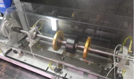
2.5.1 Rotor Test Rig
The proposed uncertainty analysis was applied to a horizontal rotating machine modeled by using 35 Timoshenko beam elements, which is shown in Figure 2.13. The rotor system is composed by a flexible steel shaft with 840 mm length and 19.05 mm diameter (E = 1.9 x 10¹¹ Pa, ρ = 8030 kg/m3, and υ = 0.3), three rigid discs D1 (node #16; 0.658 kg), D2 (node #20; 5.013 kg), and D3 (node #25; 0.658 kg), and two cylindrical hydrodynamic bearings (B1 and B2, located at the nodes #9 and #35, respectively), each one with 19.05 mm diameter and 12.8 mm length. The rotating parts take into account a proportional damping added to the matrix D (Eq. (1); Dp = γ M + β K) with coefficients γ = 5 and β = 5 x 10⁻⁶. Following the model proposed by LALANNE and FERRARIS (1998), it is assumed that the disc D2 increases the stiffness of the shaft at the disc location (elements #19 and #20; see Figure 2.13b). Special care was dedicated to the model of the disc D2 to comply with the stiffness increase due to coupling of the disc to the shaft.
optimization task involved in this application; RIUL, STEFFEN JR and RIBEIRO (1992), justify the consideration of the short nonlinear bearing theory.
a) Rotating machine.
b) FE model.
Figure 2.13 Flexible rotor used on the experimental analysis.
Experimental frequency response functions (FRFs) were measured on the rotor at stand still for the free-free end condition by applying impact forces along the horizontal direction (i.e., X direction) at the nodes #4, #11, #18, #27 and #34, separately. The response signals were measured by three accelerometers installed along the same direction of the impact forces at the nodes #4, #11, and #34, resulting fifteen FRFs. The measurements were performed by a signal analyzer, Agilent®(model 35670A), in a range from 10 to 300 Hz and steps of 0.5 Hz. Figure 2.14 compares the four simulated and experimental FRFs by considering the parameters of the rotating machine presented above. Note that the FRFs generated from the FE model are satisfactorily close to the ones obtained directly from the test rig.
#16 #20 #25
Concerning now the assembled test rig (i.e., rotor under operating condition), displacement responses are collected in the vicinity of the bearings locations (measuring planes S1 and S2; nodes #10 and #33, respectively) along the horizontal and vertical directions (X and Z, respectively).
a) Impact: node #4; sensor: node #4. b) Impact: node #11; sensor: node #11.
c) Impact: node #18; sensor: node #34. d) Impact: node #34; sensor: node #34.
Figure 2.14 Simulated (- - -) and experimental (----) FRFs
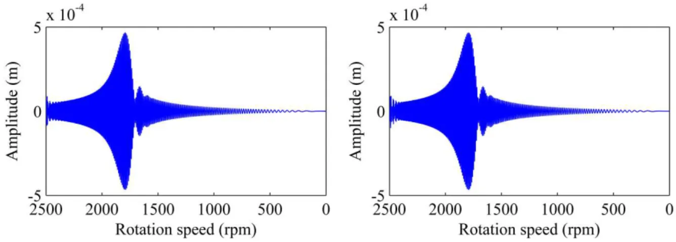
(2.16). Additionally, the simulations were performed considering the system vibrating around its equilibrium position.
a) Horizontal vibration (X direction). b) Vertical vibration (Z direction).
Figure 2.15 Simulated linear run-down responses obtained on the plane S2 (node #33)
2
11 0.007407 4.2
10k Toilk
h
(2.16)
where Toil is the oil temperature (oC). The coefficients k1 = 3.3914 and k2 = -1.1232 were determined from the measured oil viscosity.
A model updating procedure was carried out to quantify the unbalance condition and the effect caused by the coupling between the electric motor and the shaft on the dynamic behavior of the test rig. In this sense, the Differential Evolution optimization technique (STORN and PRICE, 1995) was used to determine the unknown parameters of the model. In this way, the linear and angular stiffness of the coupling (klinear and kangular added around the orthogonal directions X and Z at the node #2) and the equivalent masses/phases that should be inserted on each disc to obtain the real unbalanced condition of the test rig were determined. The entire identification process was based on time domain dynamic responses (i.e., comparison between simulated and experimental displacement responses) was performed 10 times, considering 40 individuals in the initial population of the optimizer. The objective function to be minimized is given by Eq. (2.17).
, ,
1 ,
max max
max
n exp i model i
f
i exp i
O
Οut ΟutΟut
where Outexp,i is the experimental vibration response measured directly on the test rig and
Outmodel,i is the associated response determined by the FE model. In this case, n is the number of displacement responses considered in the minimization process.
It is well known that the unbalanced masses/phases and the stiffness of the coupling do not change with the rotation speed of the rotor. Therefore, the minimization process was performed considering the rotor operating at two different rotating speeds: 1100 and 1200 rpm, separately. Consequently, the experimental displacement responses were measured on the planes S1 and S2 with the rotor operating at the same rotation speeds (full acquisition time of 0.4 sec. in steps of 0.0005 sec., approximately; measurements performed by the analyzer Agilent®model 35670A).
Table 2.5 summarizes the parameters determined in the end of the minimization process associated with the smallest value of the objective function (Eq. (2.17)) and the lower and upper limits imposed to the optimization process. Figure 2.16 compares the simulated (the last 0.4 sec. of the simulation) and experimental displacement responses of the rotor obtained on the plane S1 for the rotor operating at both considered rotation speeds. Note that the time responses generated from the FE model are not close enough to the ones obtained directly from the test rig, which can be associated with the inherent uncertainties affecting the bearings.
Table 2.5 Parameters determined by the model updating procedure
Parameters Lower limit Upper limit Optimized values
Disc D1
Unbalance (kg.m) 0 1.0 x 10⁻³ 8.3583 x 10⁻⁴
Phase (degrees) -180 180 -23.1591
Disc D2
Unbalance (kg.m) 0 1.0 x 10⁻³ 7.6299 x 10⁻⁴
Phase (degrees) -180 180 154.7898
Disc D3
Unbalance (kg.m) 0 1.0 x 10⁻³ 9.7153 x 10⁻⁴
Phase (degrees) -180 180 142.8335
Coupling klinear(N/m) 0 1.0 x 10
2 70.8333
kangular(N.rad/m) 0 1.0 x 10² 9.6127
a) Rotation speed: 1100 rpm; X direction. b) Rotation speed: 1100 rpm; Z direction.
c) Rotation speed: 1200 rpm; X direction. d) Rotation speed: 1200 rpm; Z direction.
Figure 2.16 Simulated (- - -) and experimental (----) displacement responses obtained on the plane S1.
It is worth mentioning that the simulated responses that were determined along the X direction (Figure 2.16a and Figure 2.16c) matched the ones associated with the experimental measurements. To obtain this result it was necessary to adjust the time shift between the two responses (simulated and experimental).