Transgenic, an operator for Evolutionary Algorithms
Laurence Rodrigues do Amaral
Department of Computer Science Federal University of Sao Carlos and Federal University of Goias/JataiSao Carlos - SP, Brazil Email: [email protected]
Estevam Rafael Hruschka Junior
Department of Computer Science Federal University of Sao CarlosSao Carlos - SP, Brazil Email: [email protected]
Abstract—In the 1950s and the 1960s several computer sci-entists independently studied evolutionary systems with the idea that evolution could be used as an optimization tool for engineer-ing problems. For these evolutionary-computation researchers, the mechanisms of evolution seem well suited for some of the most pressing computational problems in many fields. Ideas from Genetics are usually incorporated into evolutionary algorithms, such as: haploid crossover, mutation, diploid, inversion, gene doubling, deletion, and others. In the present study, we proposed an operator, named transgenic, for evolutionary algorithms, especially designed for Genetic Algorithms (GA). This operator is inspired by genetically modified organisms (GMOs), where important features are introduced into their genome artificially. The transgenic operator uses historical information to choose the best attributes, converging to better results faster than traditional GAs. The GA, used in this study, allows the discovery of concise, yet accurate, high-level rules (from a biological and synthetic database) which can be used as a classification system. The obtained results show that transgenic operator is promising at obtaining better of the the same results with a lower number of generations and smaller populations.
Index Terms—Genetic Algorithms, Genetic Engineering, Transgenic operator, Gene Ontology, Datamining
I. INTRODUCTION
Genetic engineering is the direct human manipulation of an organism’s genetic material in a way that does not occur under natural conditions. It involves the use of recombinant DNA techniques, but does not include traditional animal and plant breeding or mutagenesis. Any organism that is generated using these techniques is considered to be a genetically modified organism (GMO). Genetic engineering or recombinant DNA technology, transcends classical plant and animal breeding by permitting the rapid transfer of genetics traits between entirely different organisms [1].
Horizontal Gene Transfer (HGT) is a form of genetic en-gineering. There are three common mechanisms for HGT([2], [3], [4]): (1) transformation, the genetic alteration of a cell resulting from the introduction, uptake and expression of foreign genetic material (Deoxyribonucleic acid or DNA, it is a nucleic acid that contains the genetic instructions used in the development and functioning of all known living organisms and some viruses). This process is relatively common in bacteria and it is often used to insert novel genes into bacteria for experiments, or for industrial or medical applications. In molecular biology, transformation is the genetic alteration of a
cell resulting from the uptake, genomic incorporation, and ex-pression of foreign genetic material. The term transformation is also used, as a more general way, to describe mechanisms of transference of DNA in molecular Biology (that is to say, considering more than the genetic consequences). For example the production of a transgenic product as transgenic corn requires the insertion of new genetic information in the genome of the corn using the appropriate mechanism of DNA transfer;(2) transduction, the process in which bacterial DNA is moved from one bacterium to another by a bacterial virus. Packaging the desired genetic material wished in a suitable virus that is able to infect vegetables, allows that virus to modify the target bacterium. If the genetic material is DNA, it can recombine the chromosomes (it is a single piece of DNA containing many genes, regulatory elements and others) to produce recombinant cells. Nevertheless, the vegetal genomes of most viruses consist of RNA (Ribonucleic acid or RNA, it is a biologically important type of molecule), that replicates in the cytoplasm (the cytoplasm is the part of a cell that is enclosed within the plasma membrane separating the interior of a cell from the outside environment) of the infected cell. The lineage of these free infected plants will be free of virus and the inserted gene; and(3) bacterial conjugation, a process in which a living bacterial cell transfers genetic material through cell-to-cell contact [5].
Benefits presented by proponents of Genetically Modified (GM) technology include improvement in fruit and vegetable shelf-life and organoleptic quality, improved nutritional quality and health benefits in foods, improved protein and carbohy-drate content of foods, improved fat quality, improved quality and quantity of meat, milk and livestock. Other potential benefits are: the use of GM livestock to grow organs for transplant into humans, increased crop yield, improvement in agriculture through breeding insect, pest, disease, and weather resistant crops and herbicide tolerant crops, use of GM plants as bio-factories to yield raw materials for industrial uses, use of GM organisms in drug manufacture, in recycling and/or removal of toxic industrial wastes [6].
Molecular Biology has important areas that can benefit from the development and application of computer-based tech-niques. Computational approaches can be applied in the res-olution of different biology challenges such as, identification and analysis of gene expressions, comparison of sequences
(DNA, RNA and proteins), assembly of fragments, recognition of genes, determination of the structure of proteins [7] [8] and unification of the representation of gene and gene product attributes across species [9]. Due to the great amount of information and its complexity, tools based on conventional computation have shown to be limited in tackling complex biological problems. One explanation for such difficulty is the inefficiency of conventional tools in working with large volumes of data, as well as, problems with finding the optimal solution (or a good approximate solution). Following along those lines, computational intelligence (CI) techniques, such as, genetic algorithms, more and more are being used to solve problems in Molecular Biology. The growth in the use of CI techniques is due to specific characteristics such as their ability to automatically learn from data producing relevant results [8]. Based on the biological inspiration for new computational methods, several computer scientists independently studied evolutionary systems with the idea that evolution could be used as an optimization tool for engineering problems. Many au-thors propose methods using the biology inspiration, such as: Rechenberg introduced ”evolution strategies”, Fogel, Owens, and Walsh developed ”evolutionary programming”, among others. To evolutionary-computation researchers, the mecha-nisms of evolution seem well suited for some of the most pressing computational problems in many fields. Many com-putational problems require searching through a huge number of possibilities for solution [10].
Genetic Algorithms (GAs), the approach used in this work, were invented by John Holland in the 1960s and were devel-oped by Holland and his students and colleagues at the Univer-sity of Michigan in the 1960s and the 1970s. In contrast with evolution strategies and evolutionary programming, Holland’s original goal was not to design algorithms to solve specific problems, but rather to formally study the phenomenon of adaptation as it occurs in nature and to develop ways in which the mechanisms of natural adaptation might be imported into computer systems. Holland presents in the book Adaptation in Natural and Artificial Systems the genetic algorithm as an abstraction of biological evolution and gave a theoretical framework for adaptation under the GA [10].
John Holland presented four operators for the GAs, such as: selection, crossover, mutation and inversion. The selection operator chooses those chromosomes in the population that will be allowed to reproduce, and in general the chromo-somes having best fitness will be chosen to produce more offspring than the other ones. Crossover operators are re-sponsible for exchanging subparts of two selected chromo-somes, roughly mimicking biological recombination between two single-chromosome (”haploid”) organisms [10]. Mutation operators, on the other hand, randomly changes the allele values in specific locations in the chromosome [10]. The inversion operator reverses the order of a contiguous section of the chromosome, thus rearranging the order in which genes are arrayed [10].
Many new ideas were incorporated into GAs from Genetics, such as: haploid crossover, mutation, diploid, inversion, gene
doubling, deletion, dominance, translocation, sexual differen-tiation [11], and introns [12]. Mechanisms inspired by them could be potentially be put to excellent use in problem solving with GAs. Besides, the exploration of such mechanisms has only barely scratched the surface of their potential. Perhaps even more potentially significant is genetic regulation. In recent years a huge amount has been learned in the genetics community about how genes regulate one another - how they turn one another on and off in complicated ways so that only the appropriate genes get expressed in a given situation. It is these regulatory networks that make the genome a complex but extremely adaptive system. Capturing this kind of genetic adaptivity will be increasingly important as GAs are used in more complicated, changing environments [10].
Following along these ideas, we are proposing an operator for evolutionary algorithms inspired in genetically modified organisms (GMOs), specifically a transformation mechanism (section I), where important features are introduced into their genome artificially. The main features of the transgenic op-erator will be presented in the following section (II). The results and discussions are presented in sections III and IV respectively.
II. TRANSGENIC OPERATOR
We propose a transgenic operator for Evolutionary Algo-rithms. This operator is inspired by genetic engineering, where we manipulate the genetic material of individuals, adding features that we believe are important. In this sense, our approach can be seen as an elitism strategy focused on specific genes. Therefore, the proposed operator identifies relevant genes having specific values and keep these values in the next individuals’ target genes. In other words, if a gene G is identified as having strong influence in the fitness function when it has a specific value V, then, the transgenic operator will force some individuals in the next generation to have the value V in gene G.
We designed our transgenic operator to be part of a Genetic Algorithm (GA). GAs are computational search methods based on natural evolution and genetic mechanisms, simulating Dar-wins’s natural selection theory [11]. A GA can be classified as an Evolutionary Computation approach, which is a sub-area of Artificial Intelligence focused on the study of com-putational methods based on Darwin’s evolutionary theory. We implement the GA proposed by Amaral and Hruschka [13] adding the transgenic operator. The GA developed by Amaral and Hruschka was adapted from [14]. The GA in [14] was developed in GALLOPS tool [15] and it was elab-orated to generate IF-THEN classification rules in clinical databases. Fidelis et al.’s environment [15] was applied in databases whose registers were characterized by patient’s data such as age, familiar historical and a series of specific symptoms. The evolutionary environment, developed in the JavaR programming language, was adapted to work with Gene
A. Individual Representation
In our evolutionary environment, each individual is com-posed by thirty four (34) genes (one for each attribute in the GO Database, except strClass). The first gene of the individual corresponds to the first attribute (code 01) found in the database and successively until all the attribute of the database are represented. An individual example is illustrated in Figure 1.
Fig. 1. Individual representation
For every individual, the i-th gene (i=1...N) is subdivided into three subfields: weight (Wi), operator (Oi) and value
(Vi), as illustrated in Figure 1. Each gene corresponds to
one condition in the antecedent part of the rule (IF) and the individual as a whole is the rule antecedent. The weight field is an integer variable and its value must be defined between 0 and 10 (Wi=wi,j|wi,j= 0..10). It is important to say that
this weight field determines the insertion or the exclusion of the correspondent gene in the rule antecedent. If its value is less than a boundary-value this gene will not appear in the rule, otherwise the gene appears. In this work, after a preliminary parameter analysis, the value 9 was used as the boundary-value. For the weight field, we tested 7, 8 and 9 values using significance test. The details about the genetic operators and parameters will be detailed in subsection II-E. Any weight value can be used, but for the other values in this application, the GA does not converge or the results are not so good. The weight field depends of the each application. The operator field can be <or ≥. The value field is an integer or floating-point number that can vary between the minimum and maximum value found in the database for each attribute. The subdivisions of the gene can be altered by the mutation operator, using valid values.
B. Fitness Function (FF)
In general, the individual fitness quantifies its quality as a solution for the target problem. In this work, FF evaluates the quality of the rule associated to each individual. Some concepts must be explained before defining our FF. When a rule defined for the classification of a specific class C and is applied to a known case, four different types of results can be observed, depending on the class predicted by the rule and the true class of the case [16]:
• True Positive (tp) - The rule classifies the case as class
C and the case really belongs to class C;
• False Positive (fp) - The rule classifies the case as class
C but the case does not belong to class C;
• True Negative (tn) - The rule does not classify the case as class C and the case does not belong to class C;
• False Negative (fn) - The rule does not classify the case as class C but the case really belongs to class C;
Based on four possible results of a rule, the fitness function used in our evolutionary environment uses two indicators commonly used in medical domains, called sensitivity (Se) and specificity (Sp) which can be defined as follows:
Se= tp
(tp+f n) (1)
Sp= tn
(tn+f p) (2)
Using the sensitivity and specificity concepts, FF is defined as the combination of these two indicators, Se and Sp, as follows:
F itness= (Se+Sp)/2 (3) The objective is to maximize, at the same time, Se as well as Sp. In each execution, the GA works at a binary classification problem, that is, when the GA is searching for rules to a given class C, all the other classes are grouped in one unique class (not C).
C. Main aspects
As explained above (subsection II-A), the weight field determines the insertion or the exclusion of the corresponding gene (attribute) in the rule antecedent, i. e., if the weight field is bigger than 9 (value used in this work), the gene (or attribute) will be inserted in the rule antecedent. In each generation of the GA, the number of occurrences of genes (with weight field bigger than 9) of the best rules are incremented, building a historical. The Figure 2 shows the historical structure.
Fig. 2. Historical schema
The historical is composed by 35 positions, 34 integer and 1 float. The integer positions represent the 34 genes present on chromosome (described in subsection II-A). The float value storage the best fitness function value present in the population. The Figure 3 shows a historical example. In this case, the number of occurrences for the genes #2 and #17 are bigger than 0 (zero) because them appear in rules with fitness function value equal to 0.692 (best value founded in the population). The gene #2 is present in 4 (four) rules and the #17 is present in 6 (six) rules. If exists other rules with fitness function equals to 0.692 with other genes, the number of occurrences for these genes are incremented. If a new rule is analyzed and this rule have the fitness function value bigger than 0.692, all rules are deleted from the historical and the new rule is inserted in the historical.
Fig. 3. Historical example
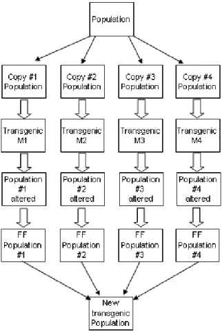
We create 4 (four) copies of the population, one for each transgenic module. After that, these individuals are changed by 4 (four) transgenic modules. The transgenic module output is the changed population. This population is evaluated and the N individuals, where N is population size, will compose the new transgenic population.
Fig. 4. Transgenic operator schema
The four modules changes the weight value of the genes, putting its bigger than 9 (for this application, the unique possible value is 10, as described in subsection II-E). The transgenic modules receive as input, a copy of the population and a list with the genes that contribute to get the most fitness function value. This list is build using the information about the genes present in the historical.
The M1 changes only one gene. For example, if the gene #17 is present at the gene list, the transgenic operator changes the weight value related to gene 17, to a value greater than 9. The M2, M3 and M4 compose the genes present in the historic list 2-2, 3-3 and 4-4, respectively. For example, if in the historical list there are the values 3, 11 and 19 and the M2
is selected, the genes 3 and 11, 3 and 19 will be changed their weight values, i.e., we will compose these values 2 to 2, and the genes 3 - 11, 3 - 19 will have their weight values placed above 9.
The M1, M2, M3 and M4 work in parallel and in the end, the four populations are composed and the top Pse are chosen, where Pse is the number of individuals of the population. The transgenic operator is not applied in all individuals of the population, in this work, the transgenic operator was applied in 10%, 30%, 50% and 70% of individuals.
D. Databases
1) Gene Ontology dataset: The Gene Ontology (GO) project is a collaborative effort addressing the need for consis-tent descriptions of gene products in different databases. The GO collaborators are developing three structured, controlled vocabularies (ontologies) that describe gene products in terms of their associated biological processes, cellular components and molecular functions in a species-independent manner. In [9] the authors defines three separate aspects to this effort:
1) Writing and maintaining the ontologies;
2) Making cross-links between the ontologies and the genes and gene products in the collaborating databases; 3) Developing tools that facilitate the creation, maintenance
and use of GO ontologies.
As stated in [9], ontologies are used mainly because they can provide a vocabulary for representing and communicating knowledge about a topic, and a set of relationships that hold among the terms of the vocabulary. They can be structurally very complex, or relatively simple. In addition, ontologies can capture domain knowledge in a way that can easily be dealt with by a computer. Also, because the terms in an ontology and the relationships between the terms are carefully defined, the use of ontologies facilitates making standard annotations, improves computational queries, and can support the construction of inference statements from the information at hand. The ontologies are developed to include all terms falling into these domains without consideration of whether the biological attribute is restricted to certain taxonomic groups. Sharing gene product names would entail tracking evolutionary histories and reflecting both ”orthologous” and ”paralogous” relationships between gene products.
It is also important to recall that GO is not a system for naming genes and proteins; it also does not attempt to describe all of biology, neither to define a nomenclature for genes or gene products. The vocabularies describe molecular phenom-ena (e.g. programmed cell death), not biological objects (e.g. proteins or genes).
The GO dataset used in our work was generated based on the GO portal (http://www.geneontology.org/) [9]. To have a dataset suitable to our goals, we built an SQL statement selecting thirty five attributes from the seqdb database (go-lite files), distributed in three classes. Table I shows the distribution of records per class. Each record in the database corresponds to a term deposited by a researcher in the GO environment. For more details see [13].
TABLE I RECORDS DISTRIBUTION
Class Number of records Percentage of records Biological Process (BP) 7,739 59.12% Cellular Component (CC) 1,293 9.88% Molecular Function (MF) 4,059 31.01%
Total 13,091 100%
2) Synthetic dataset: The synthetic dataset is composed by 4 fragments (F1, F2, F3 and F4). Each fragment has 21 (20 attributes and the class) columns and 12,000 samples. Each attribute (At) is a random integer value, with values between 0 to 9. Each sample is classified as one of 3 possible classes (1, 2 or 3) and 80% of the samples has values in the attributes that determine the class, i.e. in 20% of the samples, the value of the attributes were generated randomly. The attributes that determine the class is showed in Table II, i.e., the F1 for class 1, the attributes 3, 14 e 16 determines classes 1, 2 and 3 respectively. For the F2, the attributes are 7 and 11, 9 and 16, 2 and 17, determines classes 1, 2 and 3 respectively, and so on. Attribute values that determine the classes have to be in a certain range, for example, the class 1, the values can be 0, 1 or 2, for class 2 can be 3, 4 or 5 and for class 3 can be 6, 7 or 8. For example, for the fragment F2, 80% of the samples have the attributes 7 and 11 with values equal to 0, 1 or 2 for class 1, attributes 9 and 16 with values equal to 3, 4 or 5 for class 2 and the attributes 2 and 17 with values equal to 6, 7 or 8.
TABLE II
SYNTHETIC DATASET- RELEVANT ATTRIBUTES PER FRAGMENT AND CLASS
Fragment
F1 F2 F3 F4
Class At At At At
1 3 7 11 4 6 10 3 7 10 11
2 14 9 16 1 5 12 5 9 14 16 3 18 2 17 8 13 15 2 13 17 18
E. Genetic Operators and Parameters
To get the best environments, various configurations were tested, such as:
• Population size(Pse): 50, 100 and 200; • Generations(Ger): 10, 30 and 100; • Mutation rate:
– Individual(Mil): 10, 15, 20, 25, 30, 40, 50 and 60
– individual genes(Mig): 10, 20, 30, 40, 50, 60 and 70
• Fitness-based reinsertion strategy(Rei): elitism (Eli) and
fittest individuals survive (parents or offspring)(Fis)
• Weight field (Wgf): 7, 8 and 9;
To define the best configuration, we ran each one of the possible setting combination (based on the aforementioned list) 35 times using different random seeds and compared the obtained results considering a significance t test using
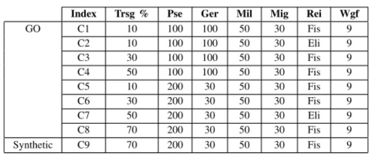
α = 0.05. Mutation is applied to the new individuals. A specific mutation operator is used for each type of gene field. During the mutation of the weight field, the new value is given by the new draw. The mutation changes the current operator field to other valid operator. We use two types of mutation: individual and individual genes. The first is the percentage of individuals of the population that will be mutated. For example: if 20% is selected and the population size is 100, 20 individual will be mutated. The second is the percentage of genes in the individuals that will be mutated. For example: if 30% is selected, 10 genes will be mutated because the individual is composed by 34 genes (subsection II-A). The Table III shows the best configurations found. As showed in Figure III, all of best configurations have mutation rate Mil equal to 50, Mig equal to 30 and the weight field equal to 9. The Index column is a key, used for identify the configuration.
TABLE III BEST CONFIGURATIONS
Index Trsg % Pse Ger Mil Mig Rei Wgf
GO C1 10 100 100 50 30 Fis 9
C2 10 100 100 50 30 Eli 9 C3 30 100 100 50 30 Fis 9 C4 50 100 100 50 30 Fis 9
C5 10 200 30 50 30 Fis 9
C6 30 200 30 50 30 Fis 9
C7 50 200 30 50 30 Eli 9
C8 70 200 30 50 30 Fis 9
Synthetic C9 70 200 30 50 30 Fis 9
III. RESULTS
For the sake of clarity, we divide the results into two parts, the next two subsections present the results obtained for GO dataset (Section III-A) and the ones obtained for the synthetic dataset (Section III-B) respectively. First, we will show the GO results.
A. GO results
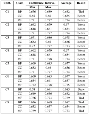
We compared our results with the results published in [13], using the same data set and the same experimentation settings, i. e., we ran our configuration 35 times using different random seeds and compared the obtained results considering a significance t test usingα= 0.05. These results are showed in Table IV. The Index column is a key ID, used for identification purposes. Table V shows the comparison, where the Result column shows whether the result is better, worse or equal than the T1 result.
TABLE IV
RESULTS PUBLISHED FORGODATASET
Index Class Confidence Interval Average Stan. Dev.
Min Max
T1 BP 0.689 0.693 0.691 0.002 CC 0.636 0.647 0.641 0.007 MF 0.758 0.769 0.763 0.007
BP class). The others configurations (C2, C3, C4, C5 and C6) obtained good results , with two class results better than T1 (for CC and MF classes) and one worse (for BP class). For the C7 and C8, only one class result better than T1 (for CC class) and two draw, for BP and MF classes.
TABLE V
COMPARISON BETWEEN TRANSGENIC AND TRADITIONALGAS FORGO
DATASET
Conf. Class Confidence Interval Average Result
Min Max
C1 BP 0.676 0.689 0.682 Tied CC 0.65 0.66 0.655 Better MF 0.771 0.777 0.774 Better C2 BP 0.662 0.679 0.67 Worst CC 0.648 0.661 0.654 Better MF 0.771 0.777 0.774 Better C3 BP 0.671 0.686 0.678 Worst CC 0.652 0.66 0.656 Better MF 0.77 0.777 0.773 Better C4 BP 0.662 0.679 0.67 Worst CC 0.648 0.661 0.654 Better MF 0.771 0.778 0.774 Better C5 BP 0.669 0.685 0.677 Worst CC 0.652 0.66 0.656 Better MF 0.771 0.777 0.774 Better C6 BP 0.669 0.685 0.677 Worst CC 0.654 0.661 0.657 Better MF 0.772 0.778 0.775 Better C7 BP 0.68 0.691 0.685 Draw CC 0.649 0.656 0.652 Better MF 0.766 0.773 0.769 Tied C8 BP 0.676 0.689 0.682 Tied CC 0.652 0.657 0.654 Better MF 0.769 0.777 0.773 Tied
During the experiments, we noticed that when the transgenic operator was present, the convergence was faster, with good results. Then, we build an experiment (named R1) designed to run for 10 generations only, having 100 individuals and the transgenic operator with 30% rate (others parameters were kept equal). The obtained results, with this new configuration, were equivalent to the ones obtained in T1 and C1. Table VI shows the results.
B. Synthetic results
We select one configuration (C9) to compare the results obtained using transgenic operator and traditional GAs. Tables VII and VIII show the results obtained by traditional GA in F1, F2, F3 and F4 datasets.
Table IX shows the results obtained by C9 configuration in F1, F2, F3 and F4 datasets. The transgenic GA obtained
TABLE VI
COMPARISON BETWEEN TRANSGENIC,TRADITIONAL AND GENERATIONS REDUCEDGAS FORGODATASET
Index Class Confidence Interval Average Result
Min Max
R1 BP 0.678 0.69 0.684 Tied CC 0.642 0.65 0.646 Tied MF 0.759 0.771 0.765 Tied T1 BP 0.689 0.693 0.691 Tied CC 0.636 0.647 0.641 Tied MF 0.758 0.769 0.763 Tied C1 BP 0.676 0.689 0.682 Tied CC 0.65 0.66 0.655 Tied MF 0.771 0.777 0.774 Tied
TABLE VII
RESULTS OBTAINED BY TRADITIONALGAINF1ANDF2DATASETS
F1 F2
Index Class Confidence Interval Avg Confidence Interval Avg
Min Max Min Max
S1 1 0.748 0.762 0.755 0.765 0.779 0.772 2 0.643 0.652 0.647 0.674 0.692 0.683 3 0.751 0.768 0.759 0.775 0.786 0.78 S2 1 0.749 0.763 0.756 0.767 0.78 0.773
2 0.638 0.646 0.642 0.668 0.685 0.676 3 0.75 0.763 0.756 0.768 0.783 0.775
TABLE VIII
RESULTS OBTAINED BY TRADITIONALGAINF3ANDF4DATASETS
F3 F4
Index Class Confidence Interval Avg Confidence Interval Avg
Min Max Min Max
S1 1 0.793 0.814 0.803 0.801 0.802 0.801 2 0.688 0.7 0.694 0.696 0.71 0.703 3 0.79 0.811 0.8 0.809 0.828 0.818 S2 1 0.791 0.811 0.801 0.802 0.821 0.811 2 0.683 0.697 0.69 0.698 0.712 0.705 3 0.786 0.804 0.795 0.809 0.829 0.819
better results in 3 classes: class 2 in F1 (0.65-0.662 against 0.638-0.646), class 2 (0.722-0.743 against 0.698-0.712) and 3 (0.834-0.856 against 0.809-0.829) in F4.
TABLE IX
RESULTS OBTAINED BY TRANSGENICGAINF1, F2, F3ANDF4DATASETS
1 2 3
Conf. Int. Avg Conf. Int. Avg Conf. Int. Avg
Min Max Min Max Min Max
F1 0.741 0.76 0.75 0.65 0.662 0.65 0.755 0.768 0.76 F2 0.773 0.798 0.78 0.67 0.689 0.67 0.783 0.806 0.79 F3 0.79 0.814 0.80 0.697 0.718 0.70 0.801 0.828 0.81 F4 0.818 0.842 0.83 0.722 0.743 0.73 0.834 0.856 0.84
TABLE X
RESULTS OBTAINED BY TRANSGENICGAINF1, F2, F3ANDF4
DATASETS WITH10GENERATIONS
1 2 3
Conf. Int. Avg Conf. Int. Avg Conf. Int. Avg
Min Max Min Max Min Max
F1 0.72 0.749 0.73 0.636 0.645 0.64 0.731 0.756 0.74 F2 0.752 0.774 0.76 0.669 0.686 0.67 0.77 0.795 0.78 F3 0.773 0.799 0.78 0.673 0.693 0.68 0.78 0.806 0.79 F4 0.796 0.824 0.81 0.692 0.711 0.70 0.8 0.825 0.81
IV. FINALREMARKS
Based on the results presented in section III, we can con-clude that, considering the employed data sets, the transgenic operator is able to increase the convergence power of the GAs, thus, it is indicated in applications where the number of gen-erations is a critical factor. For the GO dataset, the proposed operator was able to decrease the number of generations in 10 times (from 100 to 10 ie a decrease of 90%), with statistically equivalent. For synthetic dataset, the reduction was smaller than that observed for GO dataset, but still expressive. The transgenic operator reduced the number of generations in more than 60%, with statistically equivalent results.
When concerning classification accuracy, in our experi-ments, we obtained good results for GO dataset (in three classes, we obtained better results for 2 classes and 1 draw). For the synthetic dataset, the results were slightly worse. For the F4 fragment we obtained two better results and 1 draw and for F1 fragment, we obtained 1 better result and 2 draws. For F2 and F3, all results were tied.
It is important emphasize that the adopted configuration, in the construction of historical numbers and the compositions (2-2, 3-3 and 4-4) were as simple as possible. Even with this simplistic configuration, the results showed that the transgenic operator is promising, it can help in problems where the number of generations is critical.
Another important point to be mentioned is the high selec-tive pressure that the operator applies to the GA. Due to this, we need high mutation rates to escape from local optima.
For future work, we hope to further explore this line of investigation and apply the transgenic concepts to others genes of the individual, such as: operator and value. Other strategies for the construction of history will also be addressed using other metrics in the construction, such as correlations.
V. ACKNOWLEDGMENTS
Authors acknowledge the Brazilian research agencies CNPQ, CAPES and FAPESP for its financial support.
REFERENCES
[1] D. Pimentel, M. S. Hunter, J. A. LaGro, R. A. Efroymson, J. C. Landers, F. T. Mervis, C. A. McCarthy, and A. E. Boyd, “Benefits and risks of genetic engineering in agriculture,”BioScience, 1989.
[2] L. Margullis, “On the origin of mitosing cells,”J Theor Bio, 1967. [3] ——,Origin of eukaryotic cells. Yale University Press, 1970. [4] L. Margulis and D. Sagan,What is life? Simon Schuster, 1995. [5] J. A. Ruiz-Vanoye and O. Daz-Parra, “Similarities between
meta-heuristics algorithms and the science of life,”Central European Journal of Operations Research, 2010.
[6] S. G. Uzogara, “The impact of genetic modification of human foods in the 21st century: A review,”Biotechnology Advances, vol. 18, no. 3, pp. 179 – 206, 2000.
[7] J. C. Setbal and J. Meidanis,Introduction to Computacional Molecular Biology. Boston: PWS Publishing Company, 1997.
[8] P. Baldi and S. Brunak,Bioinformatics: the Machine Learning approach. MIT Press, 2001.
[9] T. G. O. Consortium, “Gene ontology: tool for the unification of biology,”Nature Genetics, 2000.
[10] M. Mitchell,An introduction to genetic algorithms. MIT Press, 1999. [11] D. E. Goldberg,Genetic Algorithms in Search, Optimization and
Ma-chine Learning. USA: Adison-Wesley, 1989.
[12] J. R. Levenick, “Inserting introns improves genetic algorithm success rate: Taking a cue from biology,” inFourth International Conference on Genetic Algorithms, 1991.
[13] L. R. d. Amaral and E. R. Hruschka, “Gene ontology classification: Building high-level knowledge using genetic algorithms,” in World Congress on Evolutionary Computation. Barcelona, Spain, 2010. [14] M. V. Fidelis, H. S. Lopes, and A. A. Freitas, “Discovery comprehensible
classification rules with a genetic algorithm,” inCongress on Evolution-ary Computation - (CEC-2000). La Jolla, CA, USA, 2000, pp. 805–810. [15] E. D. Goodman, “An introduction to gallops - the genetic algorithms optimized for portability and parallelism system,” Departament od Computer Science - Michigan State University, Tech. Rep., 1996. [16] H. S. Lopes, M. S. Coutinho, and W. C. Lima, “An evolutionary
approach to simulate cognitive feedback learning in medical domain,” in Congress on Evolutionary Computation - (CEC-2000). La Jolla, CA, USA, 2000.