Pedological mapping through integration of digital terrain models
spectral sensing and photopedology
1Mapeamento de solos pela integração de modelos digitais de terreno, pedologia
espectral e fotopedologia
José A. M. Demattê2*, Rodnei Rizzo3 e Victor Wilson Botteon2
ABSTRACT - New tools for soil mapping are needed to increase speed and accuracy of pedological mapping processes. This study integrated various technologies to map soils of the Piracicaba region in São Paulo State, Brazil. Each technology was expected to provide different information to design a detailed map. We carried out field survey and soil sampling for laboratory analysis. Initially, we conducted field visits to obtain soil patterns of a reference site. We applied the acquired patterns to an validation site, based solely on information obtained from remote sensing and cartographic databases, namely LANDSAT 7/ETM, digital elevation models (DEM) and aerial photographs. We integrated the information from each product to generate the map of the validation site, which was validated by field inspection. Textural classification using satellite imaging ranged from 21-51% of accuracy. Band 5 in the sensor showed the best performance to discriminate between clayey and sandy soils. Aerial photographs provided the best information because, besides their own inherent characteristics, they operate on a larger scale and result in a map with up to 50 polygons, while DEM reached a maximum of 30 polygons. The digital mapping technology generated 45 mapping units. Finally, the mapping efficiently separated the Latosols from the other classes; however, in some cases there was confusion in the identification of Cambisols and litholic Neosols.
Key words: Aerial photographs. Digital terrain models. Satellite images. Digital soil mapping.
RESUMO - É necessário o desenvolvimento de ferramentas que auxiliem no mapeamento de solos, a fim de agilizar o processo e melhorar sua precisão. O presente trabalho teve por objetivo integrar diversas tecnologias no desenvolvimento de um mapa de solos na região de Piracicaba-SP, Brasil. Esperava-se que cada produto fornecesse informações diferenciadas que, em conjunto, resultassem em um mapa de nível detalhado. Foram realizadas incursões a campo e amostragem de terra para análise em laboratório. Inicialmente, foram obtidos padrões de solos de uma área referência, com incursões a campo. Posteriormente, em uma área desconhecida, foram aplicados os padrões previamente conhecidos, baseado somente nos produtos sensores e bases cartográficas, a saber: imagens LANDSAT 7/ETM, modelo digital de terreno (MDT) e fotografias aéreas. A integração das informações de cada produto gerou um mapa da área desconhecida, o qual foi posteriormente validado com novas incursões a campo. A classificação textural por imagem de satélite variou de 21 a 51% de acerto. A banda 5 do sensor foi a melhor na discriminação de solos argilosos e arenosos. Em termos de contribuição, as fotografias aéreas foram o melhor produto utilizado, pois além das características a elas inerentes, tiveram escala maior, resultando em um mapa com até 50 polígonos, enquanto os MDT’s atingiram máximo de 30 polígonos. O produto do mapeamento digital gerou 45 unidades de mapeamento. Por fim, observou-se que o mapeamento separou de forma eficiente os Latossolos das outras classes, contudo, em alguns casos, houve confusão entre Cambissolos e Neossolos Litólicos.
Palavras-chave: Fotografias aéreas. Modelos digitais de terreno. Imagens de satélite. Mapeamento digital de solos.
DOI: 10.5935/1806-6690.20150053 * Autor para correspondência
1Recebido para publicação em 21/11/2013, aprovado em 29/05/2015
Pesquisa realizada com recursos da FAPESP (05/60789-0) da bolsa de Iniciação Científica do CNPq do primeiro autor
2Departamento Ciência do Solo/LSO, ESALQ/USP, Piracicaba-SP, Brasil, [email protected], [email protected] 3Centro de Energia Nuclear na Agricultura/CENA, Piracicaba-SP, Brasil, [email protected]
Rev. Ciênc. Agron., v. 46, n. 4, p. 669-678, out-dez, 2015 670
INTRODUCTION
Pedologists carry out profile description, drilling, and interpretations of landscape features as well as soil classification according to one specific system (BREGT; BOUMA; JELLINEK, 1987). The historical process described is essential as the information generated results not only in better crop management, but also in soil conservation.
According to King et al. (1999), in France, only 26% of the territory is mapped at a spatial resolution of 500 meters and 13% at 200 meters. The need for soil mapping at higher spatial resolution is even greater in larger countries such as Brazil and Australia. Fifty percent of major Australian agricultural areas (14% of the country) are mapped at a spatial resolution of 500 meters and 3% at 200 meters (MCBRATNEY; SANTOS; MINASNY, 2003). In Brazil, the existing maps are primarily the result of the RADAM /EMBRAPA project (Radar na Amazônia/Empresa Brasileira de Pesquisa Agropecuária). The maps were created on a nominal scale of 2 km. In São Paulo State, existent maps were developed by the Instituto Agronômico de Campinas (IAC) and 13% of the mapped area was made at a semi-detailed level on a scale of 1:100,000. These observations corroborate Lepsch (2013), indicating the need for detailed soil mapping in Brazil.
Remote sensing (RS) is perceived as a facilitator, since the last 30 years have witnessed advances in methods of multivariate classification, variable regionalization theory and computational tools such as geographic information systems (GIS).
This process is known as digital soil mapping (DSM), which involves creating and using spatial information obtained from field and laboratory observations linked to spatial and non-spatial systems
of inference (LAGACHERIE; MCBRATNEY; VOLTZ,
2007).
Digital mapping uses spectral pedology (DEMATTÊ; TERRA, 2014), a new technology that relates soil studies with interpretation of electromagnetic spectra. Spectroscopy is based on absorption and reflection of electromagnetic energy in different soils and distinct wavelengths according to chemical, physical and mineralogical attributes of the soil. This technology allows discriminating soil attributes (BEN-DOR et al., 2009; VISCARRA ROSSEL et al., 2011) and the information is added to digital mapping.
Similarly, aerial photographs correspond to an important tool for soil surveys because they serve as a field map-base and their interpretations are used in soil studies (LUEDER, 1959; BURING, 1960). Photopedology significantly reduces time and cost of soil surveys and
offers additional information (VINK, 1963), but has significantly been neglected in the past years.
Digital analysis of soil surface is another technique of great value for soil mapping. The influence of surface shape, slope and drainage on soil formation allows researchers to understand soil properties (MOORE; GRAYSON; LADSON, 1991). Landscape studies for soil characterization are used to relate processes that occur in soil topography, soil development and, consequently, in the environment (IRVIN; VENTURA; SLATER, 1997). There is no report in the literature of methods that combine all these techniques to define borders in a soil mapping unit (SOUZA JUNIOR; DEMATTÊ, 2008).
This study evaluated the potential to integrate geotechnical tools for soil delineation for in a highly heterogeneous site. We expect that each technique contribute differently to soil characterization and discrimination.
MATERIAL AND METHODS
Study site and soil base
The study site is in the Piracicaba region, São Paulo State, Brazil, at 22º43’S and 47º38’W. The geology is complex and variable and highlighted in the geological map of Piracicaba (IGG, 1966). The climate is Cwa (Köppen classification), tropical with dry winters and rainy summers. The main soils are Arenosol (RQ), Regosol (RL), Xanthic Ferralsol (LVA), Lixisol (PVA), and Cambisols (CX) (EMBRAPA, 2013; IUSS Working Group WRB, 2007).
Methodology
The methodology consisted of three steps: (i) calibration - assessments of an area in situ and relating the data with patterns obtained by geotechnical tools, (ii) method implementation and (iii) validation in unknown areas. Two sites were selected in the Piracicaba region, one for calibration and another for validation. The Calibration site was divided into two to ensure that more than one area was tested.
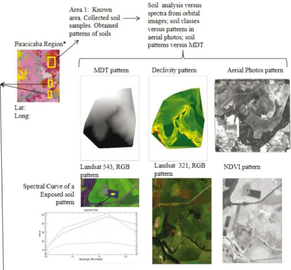
The methodological development of these phases was based on two concepts, spatial and individual. Individual evaluation (Figure 1) consists of isolated and specific characterization, not integrated - PHASE (i). At this phase, a point of the study site was analyzed in terms of slope, altitude, pixel spectrum of satellite imaging, value of the Normalized Difference Vegetation Index (NDVI) and relief aspects based on aerial photographs. This point displays the abovementioned
soil attributes. In PHASE (ii), this information is applied to the rest of the site using the pedotransfer process. Spatial evaluation takes into account the area as a continuum, seeking to combine similar individual features, generating mapping units.
Figure 1 - Flowchart exemplifying the methodology process. * Illustration of the area using Piracicaba semi-detailed soil map by Oliveira and Prado (1989)
(i) Calibration
Data collection in the field and laboratorial analyses In a specific site of the Piracicaba region, we drilled soils, collected profiles samples and conducted
Rev. Ciênc. Agron., v. 46, n. 4, p. 669-678, out-dez, 2015 672
general survey to obtain specific information and characterize the soils. We performed chemical, particle size, and morphological characterizations evaluating 12 different profiles and the most relevant soils types were Ferralsol (LVA), Regosol (RL) and Abruptic Lixisol (PV) (EMBRAPA, 2013; WRB, 2006). For the morphological description, we followed the patterns specified by Santos et al. (2005) also considering the landscape around the profiles. In addition, 178 individual samplings were carried out using an auger at 0-20, 40-60 and 80-100 cm.
The collection sites were georeferenced with high resolution GPS Trimble Pro XR. The samples were analyzed in the laboratory for particle size (CAMARGO et al., 1986), chemical attributes (pH in water and KCl, Ca2+,
Mg2+, Al3+, H+ + Al3+) and OM according to the methods
described in Raij et al. (2001).
We characterized the points based on all soil analyses (surface and subsurface) and the information was related using geotechnical tools (digital elevation models, slope, pixel spectral value, among others). This procedure allowed obtaining soil patterns. Data collection from remote sensing
We used aerial photos at the scale 1:25,000 for the qualitative characterization of landscape (relief and drainage network) (BURING, 1960; LUEDER, 1959). For the quantitative characterization, we used primary attributes obtained from digital elevation models (DEM) created by the Cartographic and Geographic Institute (IGC) at a scale of 1:10,000 (MOORE; GRAYSON; LADSON, 1991). DEM allows discriminating landscape elements of the soil formation processes. Thus, altimetric and slope maps were generated using this technique.
Images of bare soil allowed obtaining spectral characteristics of the soil surface through LANDSAT 7/ETM (Enhanced Thematic Mapper), duly corrected atmospherically and transformed to reflectance values (TANRÉ; HOBEN; KAUFMAN, 1992). Field data and soil analyses obtained from the calibration process allowed analyzing relation with the reflectance pixel value of the site and generating a spectral pattern for each soil class. Subsequently, the pattern was used in the mapping of soil texture through a supervised classification system.
In this phase, we identified the study site and its soils and their features of altitude, slope, position in the topography and spectral curve.
(ii) Implementation phase of the methodology
The implementation phase of the method was carried out in the validation area. Analyses soils in this site were based on patterns defined in phase (i).
First, the soil was mapped based only on aerial photos, called MS1. We used photopedology delineate the different areas and reliefs, determined in the mirror stereoscope allowing the delimitation of landscape units. The quality pattern of relief and drainage of the area was compared with the pattern in phase (i) to obtain the mapping units. Afterward, features of soil lines were inserted into ArcGIS 9.2 (ESRI, 2005), which allowed obtaining several polygons.
Similarly to phase (i), soil classes were related to relief and this pattern was used to classify the polygons in MS1. Another mapping was subsequently performed (MS2) based on DEM and slope. The limits of mapping units were introduced according to changes observed in these features. An indication of probable mapping units was based on comparison of patterns obtained in the calibration phase (i).
In addition to these maps, the ENVI program (RSI, 2005) obtained satellite images (LANDSAT +7/ ETM, 09/09/2010; 30 m of spatial resolution, orbit point 220/ 076 Piracicaba) with color composition, 5 Red (R), 4 Green (G), 3 Blue (B), and 3 Red, 2 Green, 1 Blue and the Normalized Difference Vegetation Index (NDVI). The NDVI refers to the interference of the vegetation cover in the image and on the spectral curve of pixels. This information was the basis for pixel identification of exposed soil (DEMATTÊ et al., 2009) and for individual evaluation of textural soil variability.
Finally, we performed a mapping (MS3) using all available resources. In this case, layers were used: (a) map of aerial photos, MS1; (b) map of DEM and slope, MS2; (c) spectral information of image pixels. Thus, the patterns of soil classes observed in the calibration phase (i) were replicated (related) in validation site area, generating MS3 mapping.
Two software programs were used simultaneously, ArcGis 9.2 and ENVI 4.4. The processed image with pixels of exposed soil was related to soil texture in ENVI software to compose the database in ArcGis. The ArcGis showed polygons obtained from aerial photographs, DEM and slope, image classified according to the textural class (individual or fragmented information, as exposed soil occurs in the entire site) and soil limits of the calibration area.
The interpretation process was semi-automatic based on the lines obtained from aerial photographs. Relief, altitude, slope, soil spectral curve and color in the images were evaluated in each polygon. In areas of exposed soil, the colors of the real composition 321RGB were related to soils in a descriptive way. Therefore, if
a color was different from another, a line was drawn. Simultaneously, in the ENVI the pixel was evaluated by the “spectral profile” that allowed visualization of the spectral curve of soil surface. The curve “shape” was compared descriptively with the orbital database.
The point was classified for similar curves. We also used spectral data to determine the textural class.
Therefore, a polygon can be classified as Ferralsol if it occurs in a plan relief, at altitude and slope compatible with the calibration site. Simultaneously, if a pixel occurs inside a polygon of exposed soil (evaluation method in the calibration phase) and shows spectral curves similar to those of Ferralsol, the polygon can be classified as such.
The identification of the probable soil belonging to the curve was obtained by means of orbital spectral curves of a database determined by Nanni and Demattê (2006) and Demattê et al. (2009). We evaluated the spectrum of the surface layer detected by satellite. To designate soil texture class in this polygon, we observed the satellite image classification in the ENVI software in areas of exposed soil. A “switch on/off” system between layers was used to relate various characteristics with a certain soil class, allowing changes in limits (DEMATTÊ et al., 2011a). Thus, lines were submitted to changes and polygons were classified with the probable soils where they belonged, generating a final mapping MS3.
(iii) Validation Phase
This phase consisted of checking accuracy and detail level achieved with the technique in the final mapping MS3 performed in the validation site. In this phase, we performed a randomization process of points in the field selecting 100 validation spots. We conducted a new soil survey in the unknown area; however, with the mapping based on patterns from the calibration phase (i). The points indicated by randomization were located in the field using a GPS. We carried out necessary observations for soil classification at each point. Subsequently, soil classification was compared at the point using geotechnical tools and in situ classification. This allowed determining the accuracy level.
RESULTS AND DISCUSSION
Spectral soil features
The average spectral curves of the top soil layer showed variations due to their constituents (Figure 2).
The difference was less significant in band 1 and all soil classes remained between 0.047 for LV and 0.076 for PV. Band 5 showed the highest reflectance variation between soils. LV showed significant differentiation in all the bands with a more pronounced concavity in the interval between bands 3 and 5, because of higher Fe content in the soil, agreeing with Nanni and Demattê (2006).
PV, RL and RQ curves showed the highest reflectance mainly in bands 5 and 7, which is related to low total Fe content and Fe particle size composition with great contribution of coarse particles (ESPIG et al., 2005). The three soils showed a grittier surface layer composed of quartz, which increases reflectance intensity in band 5 (DEMATTÊ et al., 2009). The RQ curve shape in the ascending trend agrees with observations of Demattê et al. (2009). On the other hand, curves of clayey soils, as in LV, display a “flatter” shape and have less reflectance in band 5 because of clayey feature.
Band 4 refers to the spectral range 760-900nm. The slight B4 concavity indicates the presence of Fe oxides. In this band, electronic transitions related to components of Fe oxides occur (SHERMAN; WAITE, 1985). This effect may be observed in the slight concavity occurring between bands 3 and 5, centered in band 4.
The slight difference between RQ, RL, and PV is related to textural similarity of the surface layer captured in the satellite sensor. This fact agrees with Ben-Dor et al. (2009), showing the ability of satellite imaging to capture only topsoil information without allowing its classification.
On the other hand, soils that show differences in the surface layer in terms of OM, texture, color and Fe are Figure 2 - Average spectral curves obtained from images of LANDSAT 7/ETM of soil classes evaluated
Rev. Ciênc. Agron., v. 46, n. 4, p. 669-678, out-dez, 2015 674
clayey, the lower the soil reflectance. Medium textures are more complex to estimate mainly when levels are close to the transition classes, which justifies the confusion of 27% between sandy and medium sandy classes.
Accuracy between textural sandy classes was more significant (ALVES, 2008). This fact is related to soil attributes that interfere in reflected energy. Clayey and very clayey soils of the study site have a higher content of ilmenite, magnetite and opaque minerals that absorb large amounts of energy (DEMATTÊ; TERRA, 2014).
Changes in constitution could cause the same soil classified as clayey to show different reflectance intensity. Thus, a clayey soil could be confused with medium clayey (fewer opaque minerals) or too clayey (more opaque minerals). This situation does not occur in soils with medium sandy and sandy texture.
Comparison between the RS techniques used in soil mapping
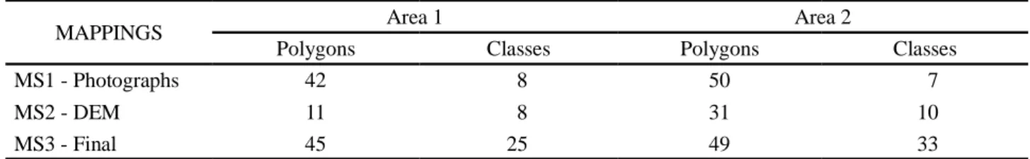
Aerial photographs generated a larger number of polygons but no significant increase in the number of soil classes as well as in number of maps obtained from DEM (Table 2). This relates to the ability of photographs to discriminate relief shapes and drainage indexes, but not to distinguish internal variations of the mapping unit such as color and texture. Demattê et al. (2001) reported similar results in which the aerial photographs showed a high discrimination level of polygons.
MS2, in turn, showed variations of altitude. This helps in the spatial diagnosis agreeing with Souza Junior and Demattê (2008). Similarly, slope levels indicate the slope percentage and areas with different slopes indicate probable differences in soils. The number of polygons obtained from these products is smaller than that obtained from the aerial photographs, because the products do not show visual information to enable further differentiations. Thus, stereoscopy provides relief volume to the researcher, differences in vegetation tones and ramp shapes, assisting in the identification of physiographic units.
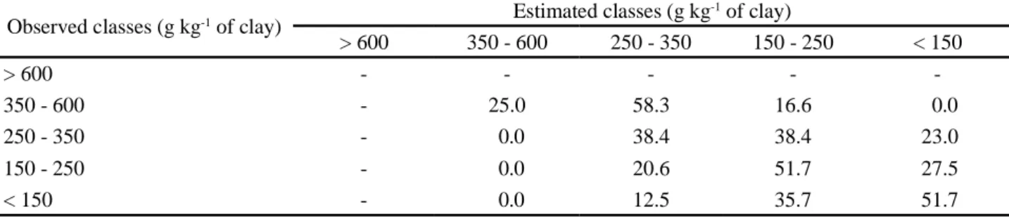
Table 1 - Estimative of surface texture mapping
Observed classes (g kg-1 of clay) Estimated classes (g kg
-1 of clay) > 600 350 - 600 250 - 350 150 - 250 < 150 > 600 - - - - -350 - 600 - 25.0 58.3 16.6 0.0 250 - 350 - 0.0 38.4 38.4 23.0 150 - 250 - 0.0 20.6 51.7 27.5 < 150 - 0.0 12.5 35.7 51.7
discriminated, as observed by Nanni and Demattê (2006). This, however, does not interfere in soil classification but in its discrimination. Interpretation of surface curves allows initial inference of probable soil characteristics, agreeing with Genú and Demattê (2012). Data on soil surface may be related to altitude, relief and affect soil classes. Estimative and spatialization of topsoil texture
In the assessment process of soil textural classes through satellite imaging, a greater confusion was observed between clayey (350-600 g kg-1) and medium
clayey (250-350 g kg-1) classes (Table 1).
In this case, 58.33% of clayey samples were classified as medium clayey. However, the opposite did not occur, i.e., there was no confusion among medium class samples with clay class. The medium texture was subdivided into medium clayey and medium sandy for evaluation purposes, a procedure that has been used in soil management (DEMATTÊ and DEMATTÊ, 2009). Franceschini et al. (2013) also reported significant differences among soils with different textures in laboratory and with hyperspectral sensing (FRANCESCHINI et al., 2015). Soil texture prediction through spectrum by terrestrial platform has shown to be more efficient (ARAÚJO et al., 2014) reaching R² 0.82. In the orbital level, values are moderate in band 0. In this case, the classifier confused the two classes with 38.46% of accuracy and confusing other 38.46% between classes. On the other hand, if the classifier considered average texture between 15-35%, the accuracy would be higher. In sandy textures, the accuracy obtained was greater and this aspect accounted for more than 50%. Genú and Demattê (2011) obtained good results in classifying soil texture from the region of Rafard, São Paulo State, Brazil, through images of satellite Aster. However, the official classification is sandy, medium, clayey, very clayey and silty (EMBRAPA, 2013).
No confusion was observed between classes of clayey and sandy textures because texture directly affects the spectral response of target (MADEIRA NETTO, 2001). The more
Merging the information obtained from MS1 and MS2 with the individual data of spectral curves allowed adding other features to the mapping units (Figure 3).
A polygon determined in aerial photos may present points (pixels) with different textural classes (DEMATTÊ, TOLEDO; SIMÕES, 2004). Therefore, the original
Table 2 - Total count of polygons and soil classes in MS1, MS2 and MS3 mappings carried out in unknown areas 1 and 2
MAPPINGS Area 1 Area 2
Polygons Classes Polygons Classes
MS1 - Photographs 42 8 50 7
MS2 - DEM 11 8 31 10
MS3 - Final 45 25 49 33
polygon would be subdivided into two classes with the limit based on DEM. The largest number of polygons was obtained in MS3 in the two areas studied (Figure 4).
The aspect described above indicates the ability of RS to generate additional information to MS3 without further fieldwork. We performed field validation to assess maps constructed, MS1, MS2 and MS3. At random points
Figure 3 - Representation of maps MS1 (soil mapping based and photopedology) and MS2 (soil mapping based on MDT and slope) for the unknown areas 1 and 2. LV, red Ferralsol; LVA, red yellow Ferralsol; PV, red lixisol; PVA, red-yellow Lixisol; CX, Cambisol; RL, Regosol, RQ, Arenosol; GX, Gleysol
Rev. Ciênc. Agron., v. 46, n. 4, p. 669-678, out-dez, 2015 676
1:50,000 and 1:100,000 publication, significantly different from the maps presented here (scale 1:25,000). In area 1, the number of polygons was 16 against 45 determined by the digital system. In area 2, there were four polygons of soils against 49 for the digital system. Semi-detailed could not have better nor similar data when compared with the digital system, because of the low scale used for that objective. On the other hand, we could start a new map from a pre-existing work on a smaller scale and, with the aid of geotechnical tools and a larger scale, achieve high improvement rates in soil mapping. The use of previous works of great importance such as Oliveira and Prado (1989) is necessary to improve mapping levels, similar to other techniques such as the DSMART software by Odgers et al. (2014).
CONCLUSION
The results show that the use of geotechnical tools allowed pedological mapping with up to 80% of accuracy in field validation. Each technique contributed with an specific information. Photopedology discriminated up to 50 polygons against 31 in DEM. Aerial photographs generated the most confortable situation for the researcher to detect relief variations in terms of DEM. Satellite images were useful in determining superficial texture of soil classes. In addition, images assisted in the evaluation of the spectral curve when compared with soil patterns in the literature. The use of all the techniques in conjunction validates the work hypothesis in which each technique Figure 4 - Representation of final soil mapping MS3, geotechnical tools (aerial photographs, MDT, slope and satellite images) for the unknown areas 1 and 2. LV, red Ferralsol; LVA, red yellow Ferralsol; PV, red Lixisol; PVA, red-yellow Lixisol; CX, Cambisol; RL, Regosol, RQ, Arenosol; GX, Gleysol; Numbers represent different types of soil mapping units
(locations), fieldwork was performed to classify the soils in situ (individual evaluation). The results were compared to soil classification using the geotechnical method. This comparison between the fieldwork and geotechnical maps (MS3) indicated 80% accuracy, which shows the high accuracy degree of the techniques for support and improvement of pre-existing maps or in the creation of new maps.
Fifty years ago, Lueder (1959) indicated that knowing an object with a sensor required assessing first each element of the product. Only at the end of the process, the researcher should gather information to generate the map. In this case, the author conceptualized the assessment method in aerial photographs that studied first the tones, current usage, drainage network, relief, erosion aspects, analysis of standards (in general) and the relationship with geomorphology. The technique presented in this study agrees with these concepts. The increased number of techniques in RS and geoprocessing shows the importance to assess components individually first: altitude, DEM patterns, satellite images, relief and gather information to obtain the results, agreeing with Demattê, Rizzo, Bortoleto (2011).
Recently, the importance of conducting detailed-level soil mappings has been highlighted on a scale compatible with that used in this work. The technologies described here could assist in the improvement of pre-existing maps of smaller scales such as the pedological map of Piracicaba that was conducted in the region by Oliveira and Prado (1989), which covers the study site. This map was made using traditional methods with base-map scale
presented their contribution. Maps generated from a single technique tend to be less detailed.
ACKNOWLEDGEMENTS
The authors wish to thank CNPQ for the scholarship granted to the first author and the Foundation for Research Support of São Paulo State (FAPESP) (05/60789-0) for the scholarship granted to the second author. We thank the Group Geotechnologies in Soil Science (Geoss; GeoCis, website:http://esalqgeocis.wix. com/geocis).
REFERENCES
ALVES, M. R. Múltiplas técnicas no mapeamento digital de solos. 2008. 159 f. Tese (Doutorado em Solos e Nutrição de Plantas) - Escola Superior de Agricultura Luiz de Queiroz, Universidade de São Paulo, Piracicaba, 2008.
ARAÚJO, S. R. et al. Improving the prediction performance of a large tropical vis-NIR spectroscopic soil library from Brazil by clustering into smaller subsets or use of data mining calibration techniques. European Journal of Soil Science, v. 65, n. 5, p. 718-729, 2014.
BEN-DOR, E. et al. Using imaging spectroscopy to study soil properties. Remote Sensing of Environment, v. 113, n. 1, p. 38-55, 2009.
BREGT, A. K.; BOUMA, J.; JELLINEK, M. Comparison of thematic maps derived from a soil map and from kriging of point data. Geoderma, v. 39, n. 4, p. 281-291, 1987.
BURING, P. The application of aerial photography in soils surveys. In: AMERICAN SOCIETY OF FOTOGRAMMETRY. Manual of photography interpretation. Washington, D.C.: American Society of Photogrammetry, 1960. cap. 11, p. 633-636.
CAMARGO, A. O. de et al. Métodos de análise química,
mineralógica e física de solos do Instituto Agronômico de Campinas. Campinas: Instituto Agronômico, 1986. 94 p. (Boletim Técnico).
DEMATTÊ, J. A. M. et al. Remote sensing in the recognition and mapping of tropical soils developed on topographic sequences. Mapping Sciences and Remote Sensing, v. 38, n. 2, p. 79-102, 2001.
DEMATTÊ, J. A. M. et al. Fotopedologia e pedologia espectral orbital associadas no estudo de solos desenvolvidos de basalto. Bragantia, v. 70, n. 1, p. 122- 131, 2011a.
DEMATTÊ, J. A. M. et al. Methodology for bare soil detection and discrimination by Landsat- TM image. The Open Journal of Remote Sensing, v. 2, p. 24-35, 2009.
DEMATTÊ, J. A. M.; RIZZO, R.; BORTOLETO, M. A. Método geotecológico integrativo na caracterização de solos
desenvolvidos de diferentes materiais de origem. Bragantia, v. 70, n. 3, p. 638 - 648, 2011.
DEMATTÊ, J. A. M.; TERRA, F. da S. Spectral pedology: a new perspective on evaluetion of soils along pedogenetic alterations. Geoderma, v. 217-218, p. 190- 200, 2014.
DEMATTÊ, J. A. M.; TOLEDO, A. M. A.; SIMÕES, M. S. Metodologia para reconhecimento de três solos por sensores: laboratorial e orbital. Revista Brasileira de Ciência do Solo, v. 28, n. 5, p. 877-889, 2004.
DEMATTÊ, J. L. I.; DEMATTÊ, J. A. M. Ambientes de produção como estratégia de manejo na cultura da cana-de-açúcar. Informações Agronômicas, n. 127, p. 10-18, 2009.
EMPRESA BRASILEIRA DE PESQUISA AGROPECUÁRIA. Centro Nacional de Pesquisa de Solos. Sistema Brasileiro de Classificação de Solos. 3. ed. Brasília, DF: EMBRAPA, 2013. 342 p.
ENVIRONMENTAL SYSTEMS RESEARCH INSTITUTE. ArcGis, software processamento de dados. 2005.
ESPIG, S. A. et al. Relação entre o fator de reflectância e o teor de Óxido de Ferro em Latossolos Brasileiros. In: SIMPÓSIO DE SENSORIAMENTO REMOTO, 12., 2005, Goiânia. Anais... Goiânia: INPE, 2005. p. 371-379.
FRANCESCHINI, M. H. D. et al. Abordagens
semiquantitativa e quantitativa na avaliação da textura do solo por espectroscopia de reflectância bidirecional no VIS-NIR-SWIR. Pesquisa Agropecuária Brasileira, v. 48, n. 12, p. 1568-1581, 2013.
FRANCESCHINI, M.H.D; DEMATTÊ, J.A.M.; TERRA, F. da S.; VICENTE, L.E.; BARTHOLOMEUS, H.; SOUZA FILHO, C.R. de. Imaging spectroscopy and accurate prediction of topsoil properties highly weathered sils: the influence of fractional vegetation cover. International Journal of Applied Earth Observation and Geoinformation, 38 (2015) 358-370. 2015.
GENÚ, A. M.; DEMATTÊ, J. A. M. Espectrorradiometria de solos e comparação com sensores orbitais. Bragantia, v. 71, n. 1, p. 82-89, 2012.
GENÚ, A. M.; DEMATTÊ, J. A. M. Prediction os soil chemical atributes using optical remote sensing. Acta Scientiarum Agronomy, v. 33, n. 4, p. 723-727, 2011.
INSTITUTO GEOGRÁFICO E GEOLÓGICO DO ESTADO DE SÃO PAULO. Folha Geológica de Piracicaba, SF 23-M300, 1966. Escala 1:100 000.
IRVIN, B. J.; VENTURA, S .J.; SLATER, B. K. Fuzzy and isodata classification of landform elements from digital terrain data in Pleasant alley. Geoderma, v. 77, n. 2-4, p. 137-154, 1997. IUSS Working Group WRB. 2007. World Reference Base for Soil Resources 2006, first update 2007. World Soil Resources Reports No. 103. FAO, Rome.
KING, D. et al. Inventaire cartographique et surveillance des sols en France. Etat d’advancement et exemples d’utilisation. Étude et Gestion des Sols v. 6, n. 4, p. 215-228. 1999.
Rev. Ciênc. Agron., v. 46, n. 4, p. 669-678, out-dez, 2015 678
OLIVEIRA, J. B.; PRADO, H. Carta pedológica de Piracicaba. Campinas: Instituto Agronômico, 1989. Escala 1:100.000. RAIJ, B. V. et al. Análise química para avaliação da fertilidade de solos tropicais. 1. ed. Campinas: Instituto Agronômico, 2001. 285 p.
RESEARCH SYSTEM INC. ENVI 4.1. Boulder: SRI, 2005. 2 CD-ROM.
SANTOS, R. D. et al. Manual de descrição e coleta de solo no campo. 5. ed. Viçosa, MG: Sociedade Brasileira de Ciência do Solo, 2005. 100 p.
SHERMAN, D. M.; WAITE, T. D. Electronic spectra of Fe+3 oxides and oxide hydroxides in the near IR to near UV. American Mineralogist, v. 70, p. 1296-1269, 1985.
SOUSA JUNIOR, J. G. A.; DEMATTÊ, J. A. M. Modelo digital de elevação na caracterização de solos desenvolvidos de basalto e material arenítico. Revista Brasileira de Ciência do Solo, v. 31, n. 1, p. 449-456, 2008.
TANRÉ, D.; HOBEN, B. N.; KAUFMAN, Y. J. Atmospheric correction algorithm for NOAA-AVHRR products: theory and application. IEEE Transactions on Geoscience and Remote Sensing, v. 30, n. 2, p. 231-248, 1992.
VINK, A. D. A. Fotografias aéreas y lãs ciências del suelo. Delf: International Training Centre for Aerial Survey, 1963. 200 p. VISCARRA ROSSEL, R. A. et al. On the soil information content of visible-near infrared reflectance spectra. European Journal of Soil Science, v. 62, p. 442-453. 2011.
LAGACHERIE, P.; MCBRATNEY, A. B.; VOLTZ, M. Digital Soil Mapping: an introductory perspective. 1. ed.. Amsterdam: Elsevier, 2007. v. 31, 668 p. (Developments in Soil Science). LEPSCH, I. F. As necessidades de efetuarmos levantamentos pedológicos detalhados no Brasil e de estabelecermos as séries de solos. Revista Tamoios, v. 9, n. 1, p. 03-15, 2013.
LUEDER, D. R. Aerial photographic interpretation: principles and applications. 1. ed. New York: MCGraw-Hill, 1959. 462 p.
MADEIRA NETTO, J. S. Comportamento espectral dos solos. In: MENESES, P.R.; MADEIRA NETTO, J. S. (Org.). Sensoriamento Remoto: reflectância de alvos naturais. Brasília: Editora UnB; EMBRAPA Cerrados, 2001. cap. 4., p.127-156.
McBRATNEY, A. B.; SANTOS, M. L. M.; MINASNY, B. On digital soil mapping. Geoderma, v. 117, n. 1-2, p. 3-52, 2003. MOORE, I. D.; GRAYSON, R. B.; LADSON, A. R. Digital terrain modeling: a review of hydrological, geomorphological and biological applications. Hydrological Processes, v. 5, p. 3-30, 1991.
NANNI, M. R.; DEMATTÊ, J. A. M. Spectral reflectance methodology in comparison to traditional soil analysis. Soil Science Society of America Journal, v. 70, p. 393-407, 2006. ODGERS, N.P. et al. Disaggregating and harmonising soil map units through resampled classification trees. Geoderma, v. 214, p. 91-100, 2014.