No part of this copyrighted work may be reproduced or used in any form or by any means - graphic, electronic or mechanical, including photocopying, recording, tape recording, web distribution, or information storage and retrieval systems - without the prior written permission of the publisher.
Preface
Major Features
With each case study, we illustrate the application of the four-step process of learning from data. The student is then asked a variety of questions that a researcher would ask when trying to summarize the results of a study.
Topics Covered
We have further enhanced the practical nature of statistics by using examples and exercises from journal articles, newspapers and our many consulting experiences. These provide students with further evidence of the practical use of statistics in solving problems that are relevant to their everyday lives.
Emphasis on Interpretation, Not Computation
In most cases, if nⱖ 30, the central limit theorem allows us to use these procedures when the population distribution is non-normal.
Changes in the New Edition
We emphasize how not considering all factors in the design phase can result in a study that fails to answer questions important to the researcher. All data sets for each exercise outcome are available at http://www.duxbury.com.
Features Retained from Previous Editions
Although the final chapter is devoted to communicating and documenting the results of the data analyses, we have incorporated many of these ideas throughout the text using the case studies.
Ancillaries
Acknowledgments
We are also indebted to Chris Franklin of the University of Georgia for her thoughtful comments on the changes required for this edition and for her discussion of the revised chapters. Special thanks go to Felicita Longnecker, Michael's wife, for her assistance in preparing the draft material and proofreading and for her help in typing the first draft of this edition.
Introduction
1 What Is Statistics?
What Is Statistics?
- Introduction
- Introduction 3 TABLE
- Why Study Statistics?
- Some Current Applications of Statistics
The results of the study may not be relevant to the general population if many of the study participants had a certain health condition. The results of the weight gain study would be of vital importance to physicians who have patients participating in the smoking cessation program.
Acid Rain: A Threat to Our Environment
It is easy, intentionally or unintentionally, to distort the truth using statistics when presenting sampling results to the uninformed. These ads often feature the numerical results of experiments comparing a new drug to an old one.
Determining the Effectiveness of a New Drug Product
Internal combustion engine fuels are also important sources of nitrogen and sulfur oxides from acid rain. The development of the Salk vaccine is not an isolated example of the use of statistics for drug testing and development.
Applications of Statistics in Our Courts
Although fewer than 200 cases of polio were reported among the 400,000 participants in the clinical trial, more than three times as many cases occurred in the group given the placebo. Statistics have thus played an important role in the development and testing of contraceptive pills, rubella vaccines, chemotherapeutic agents in the treatment of cancer and many other preparations.
Estimating Bowhead Whale Population Size
Some Current Applications of Statistics 9 estimates to determine the aboriginal subsistence whaling quota for Alaskan Es-
The researchers then applied statistical models and estimation techniques to the data obtained from the census to determine whether the Greenland population had increased or decreased since commercial whaling was stopped. The statistical estimates showed that Greenland's population was increasing at a healthy rate, indicating that stocks of large whales decimated by commercial hunting could recover after hunting ends.
Ozone Exposure and Population Density
Opinion and Preference Polls
- What Do Statisticians Do?
- Quality and Process Improvement
- Quality and Process Improvement 13 addressed how a corporation could achieve radical improvement in quality, effi-
- A Note to the Student
- Summary
We do this to raise awareness of some of the broader issues surrounding data learning in the business and scientific community. Studying the discipline of statistics requires us to memorize new terms and concepts (much like the study of a foreign language).
Supplementary Exercises
What are some of the major limitations of this study regarding the safety of helmets worn by high school players. For example, does the strength of the player's neck relate to the amount of impact transmitted to the neck and whether the player will be injured.
Collecting Data
2 Using Surveys and Scientific Studies to Gather Data
Using Surveys and Scientific Studies to
- Introduction
- Surveys 19 appropriate method to collect the data. Data collection processes include surveys,
- Surveys
- Surveys 21 Sampling Techniques
The purpose of the survey is to collect data about existing conditions, attitudes or behaviour. In this chapter we will consider some of the survey methods and designs for scientific studies.
Problems Associated with Surveys
Surveys 23 3. Using statistical techniques to adjust the survey findings to account for
Measurement problems result from the respondent not providing the information the survey seeks. The question asked to the respondent was: 'How often did you exercise in the past week?'.
Data Collection Techniques
- Surveys 25 The investigator can also monitor the interviews to be certain that the specified
- Scientific Studies 27
- Scientific Studies
- Scientific Studies 29 account. Also, the environmental conditions encountered during the experiment
In our case, we would like to avoid distorting the comparison of tire brands due to differences in the four cars. What happens if the position of the tires on the car affects tire wear.
Factorial Experiments
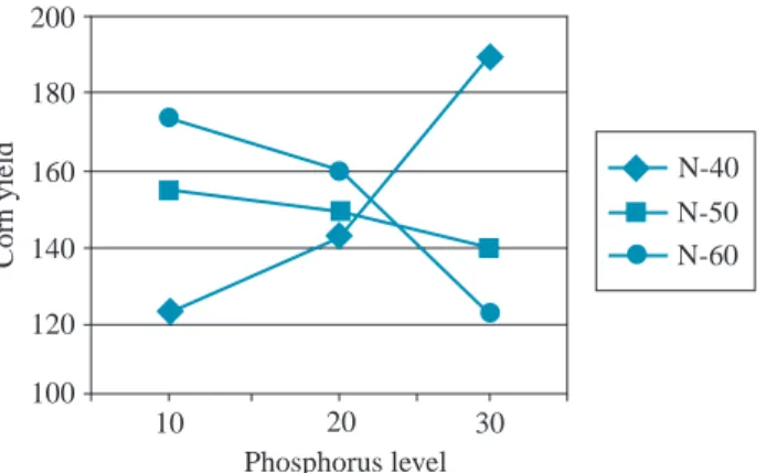
Scientific Studies 31 that 10 pounds of phosphorus with 60 pounds of nitrogen produces the maximum
However, at the 10 level of phosphorus, yield increases by 50 bushels as the level of nitrogen increases from 40 to 60. Note that the change in yield is the same at all nitrogen levels for a given change in phosphorus.
Scientific Studies 33
More Complicated Designs
Observational Studies
At the end of the study, the two groups would be compared on lung cancer and cardiovascular disease. Another possible study would be to sample a fixed number of smokers and a fixed number of nonsmokers to compare the lung cancer and cardiovascular disease groups.
Factor 1 I II III
- Data Management 35 groups of individuals followed the study plan, the observed differences between the
- Data Management: Preparing Data for Summarization and Analysis
Differences between the two groups in the observation cannot necessarily be attributed to the effect of cigarette smoking, because, for example, there may be hereditary factors that predispose to smoking and lung cancer and/or cardiovascular disease. Differences between the groups may thus be due to hereditary factors, smoking or a combination of the two.
Edit the database
- Data Management 37 a listing of the database and check it carefully to see that all numbers and characters
- Summary
It is important to preserve the source of the raw data because it is the beginning of the data trail that leads from the raw data to the conclusions of the study. A data file entered on a terminal is called a machine-readable database. A list (dump) of the database should be obtained and carefully checked against the origin of the raw data.
Summarizing Data
3 Data Description
Introduction
Our biggest problem is organizing, summarizing and describing this data - that is, making sense of the data. Good descriptive statistics allow us to make sense of the data by reducing a large set of measurements to a few summary measures that give a good, rough picture of the original measurements.
Data Description
- Calculators, Computers, and Software Systems 41 In situations in which we are concerned with statistical inference, a sample
- Calculators, Computers, and Software Systems
- Describing Data on a Single Variable: Graphical Methods 43 Throughout the textbook, we will use computer software systems to do some
- Describing Data on a Single Variable: Graphical Methods
- Describing Data on a Single Variable: Graphical Methods 45
- Describing Data on a Single Variable: Graphical Methods 49 The data of Table 3.2 have been organized into a frequency table, which
- Describing Data on a Single Variable: Graphical Methods 51
- Describing Data on a Single Variable: Graphical Methods 53
- Describing Data on a Single Variable: Graphical Methods 55
- Describing Data on a Single Variable: Graphical Methods 57 Data Display
For each variable category, draw a rectangle with a height equal to the frequency (number of observations) in the category. When the number of class intervals is too small, most patterns or trends in the data are not shown; see Figure 3.8(a).
Character Stem-and-Leaf Display
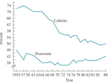
Describing Data on a Single Variable: Graphical Methods 61 Sometimes it is important to compare trends over time in a variable for two
The width of the intervals between time points reflects the fact that Catholics were not asked about their church attendance every year. The title should immediately inform the viewer of the point of the graph and draw the eye to the most important elements of the graph.
Describing Data on a Single Variable: Graphical Methods 63 EXERCISES Basic Techniques
Although fluoride levels are measured more than once a day, these data represent early morning readings for the 25 days sampled. If one of these 25 days were chosen at random, what would be the chance (probability) that the fluoride reading would be greater than .90 ppm.
Describing Data on a Single Variable: Graphical Methods 65
If you were transferred by your employer to one of the 24 cities, what is the probability that your city tax would be more than €900? The following table contains expenditures (in billion dollars) for the Department of Defense since 1980 and expenditures as a percentage of gross domestic product (% GNP).
Describing Data on a Single Variable: Graphical Methods 67
Construct a relative frequency histogram plot for the homeownership data given in the table for 1985 and 1996. How might Congress use the information in these plots to write tax laws that allow large homeownership tax deductions.
Describing Data on a Single Variable: Measures of Central Tendency 69
Describing Data on a Single Variable: Measures of Central Tendency
Identifying the condition of Example 3.1 was quite easy because we were able to count the number of times each measurement occurred. Condition is also commonly used as a measure of popularity, reflecting central tendency or opinion.
Describing Data on a Single Variable: Measures of Central Tendency 71 The second measure of central tendency we consider is the median
Because the actual values of the measurements are unknown, we know that the median occurs in a given class interval, but we do not know where to find the median within the interval. Solution Let the cumulative relative frequency for the class be equal to the sum of the relative frequencies for class 1 through class j.
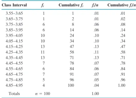
Describing Data on a Single Variable: Measures of Central Tendency 73 contains the median, we must find the first interval for which the cumulative
The sample mean formula for grouped data is only slightly more complicated than the formula just presented for ungrouped data. Therefore, when the sample measurements are known, the formula for ungrouped data should be used.
Describing Data on a Single Variable: Measures of Central Tendency 75 EXAMPLE 3.6
The median of subsets cannot be combined to determine the median of the entire data set. The means of subsets can be combined to determine the mean of the entire data set.
Describing Data on a Single Variable: Measures of Central Tendency 79
In particular, the yield of apple trees is directly related to the nitrogen content of the apple leaves and must be carefully monitored to protect the trees in an orchard. Average the three group means, the three group means, and the three group modes, and compare your results with those of part (b).
Describing Data on a Single Variable
Measures of Variability
Describing Data on a Single Variable: Measures of Variability 83 and the ranking of a person in comparison to the rest of the people taking an
Thus, approximately half of the subjects in the study have a serum cholesterol level of less than 196.5 and half greater than 196.5. To illustrate the calculations, suppose we want to determine the 80th percentile of the cholesterol data—that is, the cholesterol level such that 80% of the people in the population have a cholesterol level less than this value, Q(.80) .
Describing Data on a Single Variable: Measures of Variability 85
In fact, the IQR can be very misleading when the data set is highly concentrated around the mean. In fact, the IQR only measures the distance needed to cover the middle 50% of the data values and, therefore, completely ignores the spread in the bottom and top 25%.
Describing Data on a Single Variable: Measures of Variability 87
We then have s denoting the sample standard deviation and denoting the corresponding population standard deviation. Using the sum of the squared deviations column, we find the sample variance to be s2⫽兺i(yi⫺y¯)2.
Describing Data on a Single Variable: Measures of Variability 89 EXAMPLE 3.10
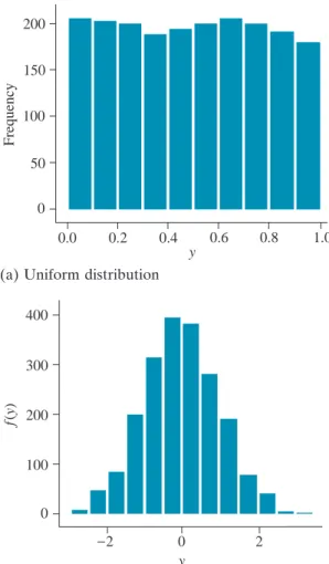
We calculated the mean and standard deviation for each of the five data sets (not given), and these are shown next to each frequency distribution. We also calculated the percentage of measurements that are within one standard deviation of the mean.
Describing Data on a Single Variable: Measures of Variability 91
If we are going to make a mistake (as we must with any approximation), it is best to overestimate the sample standard deviation so that it does not lead us to believe that there is less variability than may be the case. Calculate the mean, variance, and standard deviation of the percentage of income spent on food.
Describing Data on a Single Variable: Measures of Variability 93 Although there will not always be the close agreement found in Example
Count the percentages of squares that fall in each of the three intervals and compare these percentages with the corresponding percentages given by the empirical rule. Calculate the percentage of buses that fall in each of the three intervals and compare these percentages with the corresponding percentages given by the empirical rule.
Describing Data on a Single Variable: Measures of Variability 95
Generate a graph of the time series of mercury concentrations and plot the lines for both sites on the same graph. When comparing the center and variability of the two sites, should the years 1969–1972 be used for site 2.
The Boxplot
Let the lower quartile be the mean of the set of values consisting of the smallest values. Let the upper quartile be the mean of the set of values consisting of the largest values.
The Boxplot 99
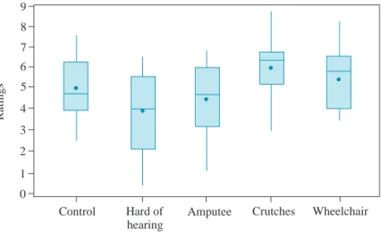
Filter C has a larger mean than both filters A and B, but less variability than A, except for two very small values obtained using filter C. Construct a box plot and describe the shape of the number distribution of persons donating blood.
Summarizing Data from More Than One Variable 101
Summarizing Data from More Than One Variable
A bar chart extension provides a convenient method of displaying data from a pair of qualitative variables. A second extension of the bar graph provides a convenient method of displaying the relationship between a single quantitative variable and a qualitative variable.
Summarizing Data from More Than One Variable 103
Each point on the field represents an operator with a certain starting salary and years of experience. An examination of Figure 3.32(a) shows that the number of attacks prior to the start of clinical trials shows similar patterns for the two groups of patients.
Summarizing Data from More Than One Variable 107
Make a percentage comparison based on the row totals and use this to describe the data. We list two measures of the money supply in the United States, M2 (private checking deposits, cash, and some savings) and M3 (M2 plus some investments), which are given here for 20 consecutive months.
Summary 109
Summary
Key Formulas
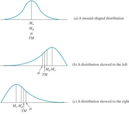
What does the ratio of mean to median indicate about the shape of the data. What does the ratio of mean to median indicate about the shape of the data.
Tools and Concepts
4 Probability and Probability Distributions
Probability and Probability
Distributions
- How Probability Can Be Used in Making Inferences
- How Probability Can Be Used in Making Inferences 123 to assess the degree of accuracy to which the sample mean, sample standard
- Finding the Probability of an Event 125 tions. For example, the director of a state welfare agency who estimates the
- Finding the Probability of an Event
- Maximum value: 9
- Finding the Probability of an Event 127 25 32 70 15 96 87 80 43 15 77 89 51 08 36 29 55 42 86 45 93 68 72 49 99 37
- Basic Event Relations and Probability Laws
- Basic Event Relations and Probability Laws 129 The concept of mutually exclusive events is used to specify a second property
- Conditional Probability and Independence 131
- Conditional Probability and Independence
- Conditional Probability and Independence 133 EXAMPLE 4.2
These definitions, along with the definition of the complement of an event, formalize some simple concepts. The vertical bar in the expression P(F兩brand policy) represents the phrase ``given that'' or simply ``given''. Thus the expression is read 'the probability of the incidentF given the fire policy of the incident. ''.
- Conditional Probability and Independence 135
- Bayes’ Formula
- Bayes’ Formula 137 Evaluation of test results is as follows
- Bayes’ Formula 139
- Variables: Discrete and Continuous 141
- Variables: Discrete and Continuous
- Probability Distributions for Discrete Random Variables
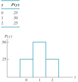
- Probability Distributions for Discrete Random Variables 143 Section 4.2 and let y be the number of heads observed. Then y can take the values
- A Useful Discrete Random Variable
Determine the probability of choosing two of the three firms that are on better ground. The relevance of the probability distribution to statistical inference will be highlighted when we discuss the probability distribution for the binomial random variable.
The Binomial
- A Useful Discrete Random Variable: The Binomial 145
- A Useful Discrete Random Variable: The Binomial 147 For n 3,
- A Useful Discrete Random Variable: The Binomial 151 procedure for obtaining approximate values to the probabilities we need in making
- A Useful Discrete Random Variable: The Binomial 153
- Probability Distributions for Continuous Random Variables
- Probability Distributions for Continuous Random Variables 155 value of y (as was done for a discrete random variable) and retain the property
- A Useful Continuous Random Variable
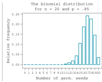
The probability of five being observed in a sample of five is shaded in the figure. Using a computer software program, we can generate the probability distribution for the number of seeds that germinate in the sample of twenty seeds, as shown in Figure 4.4.
The Normal Distribution
A Useful Continuous Random Variable: The Normal Distribution 159
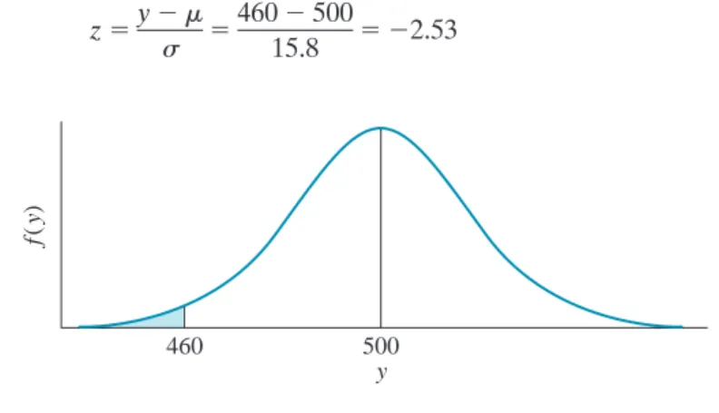
To determine the probability that a measurement will be less than some value, we first calculate the number of standard deviations away from the mean using the formula. For the normal distribution of Example 4.12 with 애 20 and 2, find the probability that it will be less than 16.
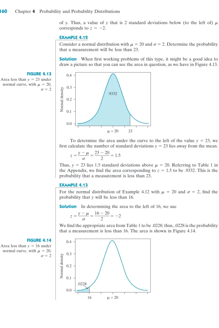
A Useful Continuous Random Variable: The Normal Distribution 161 EXAMPLE 4.14
An important aspect of the normal distribution is that we can easily find the percentiles of the distribution. To find the percentiles of the standard normal distribution, we reverse the use of Table 1.
A Useful Continuous Random Variable: The Normal Distribution 163 Suppose we wanted to determine the 80th percentile of a population having a
An analysis of income tax returns from the previous year indicates that for a given income classification, the amount of money owed to the government over and above the amount paid in estimated tax receipts for the first three payments is approximately normally distributed with a mean of $530 and a standard deviation of $205. Thus, 25% of the tax returns in this classification exceed $667.35 in the amount owed to the government.
A Useful Continuous Random Variable: The Normal Distribution 165
What is the probability that the time elapsed between submission and repayment will exceed 50 days. An exclusive club wants to invite those who scored in the top 10% on the College Board to join.
Random Sampling
Random Sampling 167 random manner can be determined, and we can use these probabilities to make
Thus, if we wanted to select a random sample of n 10 measurements from a population containing 100 measurements, we could label the measurements in the population from 0 to 99 (or 1 to 100). Solution Assuming that a list of all the households in the community is available (such as a telephone directory), we can label the households from 0 to 849 (or, equivalently, from 1 to 850).
Random Sampling 169
Assume that a sample of 25 women is needed for the study, and use Table 13 in the Appendix to determine which women should be asked to participate in the study. There are 230 precincts in the city and you must randomly select 50 registered voters from each precinct.
Sampling Distributions 171
Sampling Distributions
Note that the distribution is symmetrical with a mean of 6.5 and a standard deviation of approx. 2.0 (the area divided by 4).
Sampling Distributions 173 Example 4.19 illustrates for a very small population that we could in fact
Sampling Distributions 175
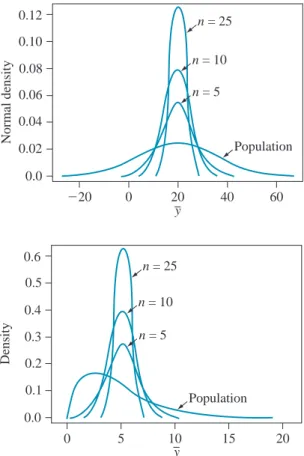
Central Limit Theorem for y
- Sampling Distributions 177 FIGURE 4.22
- Sampling Distributions 179 known either. The important point to remember is that the sampling distribution
We note that even for a very small sample size, n10, the shape of the sampling distribution of y is very similar to that of a normal distribution. If the population is highly skewed, the sampling distribution for y will still be skewed even for n 30.
Central Limit Theorem for 兺 y
- Sampling Distributions 181
- Normal Approximation to the Binomial
- Normal Approximation to the Binomial 183 The binomial random variable y is the number of successes in the n trials. Now,
The form of the Central Limit Theorem for the sample median and sample standard deviation is somewhat more complex than for the sample mean. What is the mean and standard deviation of the total amount, in g/m, of nitrogen oxide in the exhaust for the fleet.