Inferences on weather extremes and weather-related disasters: a review of statistical methods

(1)

www.clim-past.net/8/265/2012/ doi:10.5194/cp-8-265-2012

of the Past

Inferences on weather extremes and weather-related disasters:

a review of statistical methods

H. Visser1and A. C. Petersen1,2,3

1_{PBL Netherlands Environmental Assessment Agency, The Hague, The Netherlands}

2_{Centre for the Analysis of Time Series, London School of Economics and Political Science (LSE), London, UK} 3_{Institute for Environmental Studies (IVM), VU University, Amsterdam, The Netherlands}

Correspondence to:H. Visser (hans.visser@pbl.nl)

Received: 23 August 2011 – Published in Clim. Past Discuss.: 16 September 2011 Revised: 9 December 2011 – Accepted: 20 December 2011 – Published: 9 February 2012

Abstract. The study of weather extremes and their impacts, such as weather-related disasters, plays an important role in research of climate change. Due to the great societal con-sequences of extremes – historically, now and in the future – the peer-reviewed literature on this theme has been grow-ing enormously since the 1980s. Data sources have a wide origin, from century-long climate reconstructions from tree rings to relatively short (30 to 60 yr) databases with disaster statistics and human impacts.

When scanning peer-reviewed literature on weather ex-tremes and its impacts, it is noticeable that many different methods are used to make inferences. However, discussions on these methods are rare. Such discussions are important since a particular methodological choice might substantially influence the inferences made. A calculation of a return pe-riod of once in 500 yr, based on a normal distribution will deviate from that based on a Gumbel distribution. And the particular choice between a linear or a flexible trend model might influence inferences as well.

In this article, a concise overview of statistical methods applied in the field of weather extremes and weather-related disasters is given. Methods have been evaluated as to station-arity assumptions, the choice for specific probability density functions (PDFs) and the availability of uncertainty infor-mation. As for stationarity assumptions, the outcome was that good testing is essential. Inferences on extremes may be wrong if data are assumed stationary while they are not. The same holds for the block-stationarity assumption. As for PDF choices it was found that often more than one PDF shape fits to the same data. From a simulation study the con-clusion can be drawn that both the generalized extreme value

(GEV) distribution and the log-normal PDF fit very well to a variety of indicators. The application of the normal and Gumbel distributions is more limited. As for uncertainty, it is advisable to test conclusions on extremes for assumptions underlying the modelling approach. Finally, it can be con-cluded that the coupling of individual extremes or disasters to climate change should be avoided.

1 Introduction

(2)

(Kharin and Zwiers, 2005; Tebaldi et al., 2006; Orlowsky and Seneviratne, 2012).

In scanning the peer-reviewed literature on weather ex-tremes and impacts, we noticed that many different methods are used to make inferences on extremes. However, discus-sions on methods are rare. We name Katz et al. (2002) in the field of hydrology and Katz (2010) in the field of climate change research. Zhang at al. (2004) study the detection of three types of trends in extreme values, based on Monte Carlo simulations. A third example is that of Wigley (2009) and Cooley (2009), where the use of linear trends and normal distributions (Wigley) is opposed to the use of extreme value theory with time-varying parameters (Cooley). Clearly, the calculation of a return period of, say, once in 500 yr, based on a normal distribution will deviate from that based on a gen-eralized extreme value (GEV) distribution. In other words, the specific choice of methods (here the shape of probability density functions or PDFs in short) might influence the infer-ences made on these extremes. Another example is the par-ticular choice of a trend model to highlight temporal patterns in extreme-weather indicators. Conclusions based on an OLS straight line might differ from those made by more flexible trends. And the inclusion or exclusion of uncertainty infor-mation may influence inferences. A rising trend or increasing return periods are not necessarily statistically significant.

In this article, we will review the statistical methods used in the peer-reviewed literature. First, we will give a concise overview of methods applied. These methods deal with the computation of return periods of extremes, chances of cross-ing a pre-defined high (or low) threshold, the estimation of a trend in weather indicators (number of warm and cold days, annual maximum of 1-day/5-day precipitation, global num-ber of floods, etc.) or the comparison of PDFs over different periods in time.

Next to this overview we will discuss a number of method-ological aspects. We will discuss (i) the assumption of a sta-tionary climate when making inferences on extremes, (ii) the choice of (extreme value) probability distributions for the data at hand, (iii) the availability of uncertainty information and (iv) the coupling of weather or disaster statistics to cli-mate change. As for point (iv) we will pay attention to meth-ods in the peer-reviewed literature and to the way these re-sults are assessed by the Intergovernmental Panel on Climate Change (IPCC).

There are two aspects of weather extremes and their im-pacts (disasters) which willnotbe dealt with in this methods review. The first aspect concerns the quality of the data, and more specifically, methods for testing the quality of data and correcting them, if necessary. For homogeneity issues the reader is referred to Aguilar et al. (2003) and Klein Tank et al. (2009). For the reliability of disaster statistics please refer to Gall et al. (2009).

The second methodological aspect not dealt with, is that of methods for detecting anthropogenic influences in climate or disaster data. For detection studies in relation to extremes

please refer to Hegerl and Zwiers (2007), Zwiers et al. (2011) and Min et al. (2011). For a review on detecting climate change influences in disaster trends, the reader is referred to H¨oppe and Pielke (2006) and Bouwer (2011). We fur-ther note that we will use the term “climate change” in the general sense, thus, climate change both due to natural and anthropogenic influences (unless denoted otherwise).

The contents of this article are as follows. In Sect. 2, we will give a concise description of how inferences on extremes are made in the peer-reviewed literature. Then, we will dis-cuss these methods in Sect. 3 through 6 with respect to four aspects: the assumption of a stationary climate (Sect. 3), as-sumptions on probability distributions (Sect. 4), the use of uncertainty information (Sect. 5) and the coupling of ex-tremes to climate change (Sect. 6). Conclusions are given in Sect. 7. A number of statements throughout this article will be illustrated by an analysis of annual maxima of daily maximum temperatures for station De Bilt in the Netherlands (TXXt; Figs. 1, 4 and 6).

2 Methods for making inferences on extreme events and disasters

2.1 Preliminaries

There is a diverse use of terminology in the fields of cli-mate change research and disaster risk management. Terms used in the literature comprise weather or climate extremes, weather or climate extreme events, weather or climate indica-tors, weather or climate extreme indicators and indices of ex-tremes. As for disasters, any type of weather-related disasters can be analysed (floods, droughts, heat waves, hurricanes, etc.). Mostly, three types of disaster burden are presented in the literature: economic losses, the number of people killed and the number of people affected. For details see Guha-Sapir et al. (2011). The general term that is used throughout this article, is “extreme indicator”.

Extreme indicators can be constructed from underlying data (mostly daily data) by computing block extremes or threshold extremes. Block extremes are gained by taking highest (or lowest) values in a block of observations. In most cases seasonal or annual blocks are taken. Examples are the annual maximum value of daily maximum temper-atures (TXXt), the annual maximum value of one- or

five-day precipitation totals (RX1Dt, RX5Dt)or the annual

(3)

can be found in Alexander et al. (2006) or the ECA website http://eca.knmi.nl/indicesextremes/indicesdictionary.php.

Block extremes are often modelled by applying the gen-eralized extreme value (GEV) distribution. Also normal or log-normal distribution can be chosen. For a description of these methods please see Coles (2001, Chapters 3 and 6) and Katz et al. (2002), and for a description in the context of Bayesian statistics see Renard et al. (2006).

Threshold extremes, also denoted as peaks over thresh-old (POT), are gained by taking exceedances of a predefined threshold. Here, one can be interested in the number of ex-ceedances of that threshold, as in the number of summer days or tropical nights, or in the positive differences between data within a block and the threshold chosen (the excesses). Gen-erally, excess variables are modelled by applying the gener-alized Pareto distribution (GPD). For a description of these methods take note of Coles (2001, Chapters 4 and 5), Katz et al. (2002) and Coelho et al. (2008). For a description in the context of Bayesian statistics please see Renard et al. (2006). The frequency of exceedances may be analysed by a non-homogeneous Poisson process (Caires et al., 2006) or by a Poisson regression model (Villarini et al., 2011).

2.2 Stationarity and trend methods

At the basis of any analysis of extreme indicators lies the es-timation of trends1. Trends play a key role in judging if the data at hand arestationary, i.e. if the data follow a stochastic process for which the PDF does not change when shifted in time (or space). Consequently, parameters such as the mean and variance do not change over time (or position) for a sta-tionary process. Loosely formulated, stationarity means that “the data” are stable over time: no trends, breaks, shocks, ramps or changes in variance over time. Methods for as-sessing stationarity are given by Diermanse et al. (2010) and Villarini et al. (2011) and references therein.

Once a choice for stationarity has been made, trends can be estimated as such or as part of a specific non-stationary time-series approach. Examples of the latter approach are (i) making the location parameter of a GEV distribution time-varying in a certain pre-defined way (e.g. Katz et al., 2002), or (ii) making the threshold in a GPD analysis time-varying (e.g. Coelho et al., 2008).

1_{Harvey (2006) gives two definitions for “trend”. In much of}

the statistical literature a trend is conceived of as that part of a se-ries which changes relatively slowly (smoothly) over time. Viewed

in terms ofprediction, a trend is that part of the series which, when

extrapolated, gives the clearest indication of the future long-term movements in the series. In many situations these definitions will overlap. But not in all situations. In case of data following a random walk, the latter trend definition does not lead to a smooth curve. Typical examples of the first definition are splines, LOWESS smoothers and Binomial filters. Typical example of the second defi-nition is the IRW trend model in combination with the Kalman filter (examples shown in Figs. 1, 4 and 6).

The choice of a specific trend model is not a trivial one. If we scan the climate literature on trend methods, an enormous amount of models arises. We found the fol-lowing trend models or groups of models (without being complete): low pass filters (various binomial weights; with or without end point estimates), ARIMA models and vari-ations (SARIMA, GARMA, ARFIMA), linear trend with OLS, kernel smoothers, splines, the resistant (RES) method, Restricted Maximum Likelihood AR(1) based linear trends, trends in rare events by logistic regression, Bayesian trend models, simple Moving Averages, neural networks, Struc-tural Time-series Models (STMs), smooth transition models, Multiple Regression models with higher order polynomials, exponential smoothing, Mann-Kendall tests for monotonic trends (with or without correction for serial correlations), trend tests against long-memory time series, robust regres-sion trend lines (MM or LTS regresregres-sion), Seidel-Lanzante trends incorporating abrupt changes, wavelets, Singular Spectrum Analysis (SSA), LOESS and LOWESS smoothing, Shiyatov corridor methods, Holmes double-detrending meth-ods, piecewise linear fitting, Students t-test on sub-periods in time, extreme value theory with a time-varying location pa-rameter and, last not but least, some form of expert judgment (drawing a trend “by hand”). See Mills (2010) and references therein for a discussion.

This long list of trend approaches holds for trends in cli-mate data in general. However, the number of trend models applied to extreme indicators, appears to be much more lim-ited. The trend model almost exclusively applied, is the OLS straight line. This model has the advantage of being simple and generating uncertainty information for any trend differ-ence [µt -µs] (indices “t” and “s” are arbitrary time points

within the sample period)2. Examples of OLS trend fitting are given by Brown et al. (2010). They estimate trends in 17 temperature and 10 precipitation indices (all for extremes) at 40 stations. Their sample period is 1870–2005. Further-more, Brown et al. (2010) analyse the sensitivity of their re-sults with respect to the linearity assumption. To do so, they splitted the sample period in two parts of equal length and estimated the OLS trends on these two sub-periods.

Other examples of OLS linear trend fits can be found in Klein Tank et al. (2006) and Alexander (2006), albeit that the significance of the trend slope is estimated differently. Klein Tank et al. (2006) apply the Student’s t-test, while Alexander et al. (2006) apply Kendall’s tau-based slope estimator along with a correction for serial correlation according to a study of Wang and Swail (2001). Karl et al. (2008, Appendix A)

2_{The OLS regression model reads as y}

t=µt+εt= a + b*t +εt

, with “a” the intercept, “b” the slope of the regression line andεt

a noise process. Now, the variance of any trend differential [µt

-µs] follows from var(µt−µs)= var(bˆ * (t-s) ) = (t-s)2 * var(b)ˆ .

Note 1: this variance estimate is only unbiased if the residuals are normally distributed and not serially correlated. Note 2: some

au-thors estimatebˆusing Sen’s estimator. This estimator is more robust

(4)

choose linear trend estimation in combination with ARIMA models for the residuals. This is another way of correcting for serial correlation.

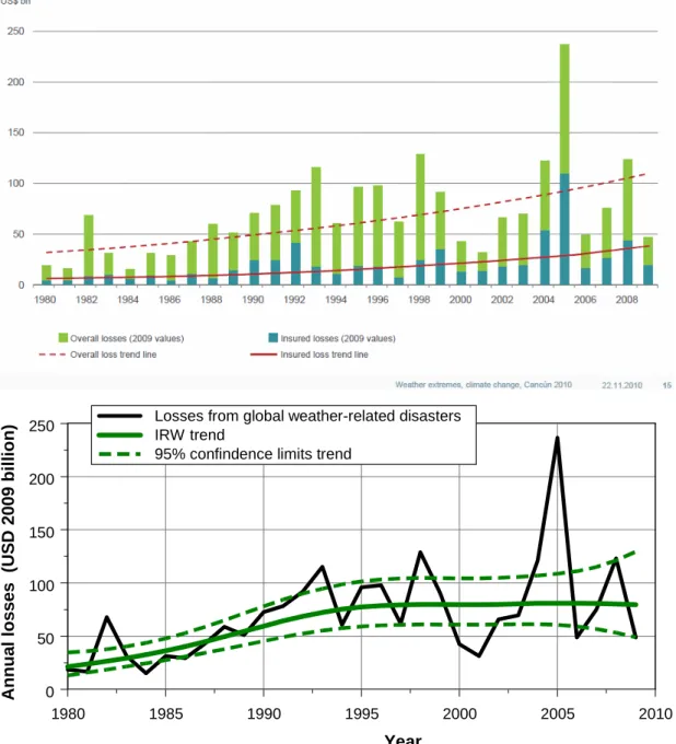
In the field ofdisaster studiesOLS trends are the dominant method, albeit that the original data are log-transformed in most cases. See Pielke (2006, Figs. 2 and 3) or Munich Re (2011, p. 47) for examples. Another trend method in this field is the moving average trend model where the flexibility is influenced by the length of the averaging window chosen. See Pielke (2006, Fig. 5) for an example. We only found one example where the GPD distribution with time-varying parameters was applied to economic loss data due to floods in the USA (Katz, 2002).

Occasionally, other trend approaches for extreme indica-tors are reported. Frei and Sch¨ar (2001) apply logistic re-gression to time series of very rare precipitation events in the Alpine region of Switzerland. They include a quantifica-tion of the potential/limitaquantifica-tion to discriminate a trend from the stochastic fluctuations in these records. Visser (2005) applies sub-models from the class of STMs, in combination with the Kalman filter, to estimate trends and uncertainty in weather indicators where trends may be flexible. The mea-sure of flexibility is estimated by ML optimization. Klein Tank et al. (2006) use the LOWESS smoother to highlight trend patterns in extreme weather indicators (their Figs. 3, 4, 6 and 7). Tebaldi et al. (2006) do not apply any specific trend model but show increases or decreases over two distant 20-yr periods: indicator differences between 2080–2099 and 1980– 1999, and between 1980–1999 and 1900–1919 (their Figs. 3 and 4). Hu et al. (2012) apply Mann-Kendall tests with cor-rection for serial correlation (no actual trend estimated in this approach).

Finally, some authors acknowledge that the use of a spe-cific trend model, along with uncertainty analysis, may lead to deviating inferences on (significant) trend changes. There-fore, they chose to evaluate trends usingmore than one trend

model. For example, Moberg and Jones apply two

differ-ent trend models to the same data: the OLS trend model and the resistant (RES) model. Subsequently, they evaluate all their results with respect to these two trend models. Even more methods are evaluated by Young et al. (2011). They es-timate five different trend models to 23-yr wind speed and wave height data and evaluate uncertainty information for each model (their supporting material). We note that the application of more than one trend model to the same data has been published more often (not specifically for the eval-uation of extremes). The reader is referred to Harvey and Mills (2003) and to Mills (2010) with references therein.

2.3 Return periods

If a particular analysis deals with extreme indicators, based on block extremes, return periods or the chance for cross-ing a pre-defined threshold can be calculated from the spe-cific PDF chosen. These chancespt, withtsome time point

within the sample period, follow directly from the PDF. Av-erage return periodsRt follow simply by taking the inverse

of pt. An example of return periods is given in Fig. 4 of

IPCC-SREX (2011).

A variant is the so-called x-year return period, with x some fixed number (often 20 in the literature). If we de-note an extreme indicator by It, a 20-yr return period,

de-noted asI_t20, stands for an indicator value in year t which is crossed once in 20 yr, on average. In fact,I_t20 stands for the 95 percentile of the PDF at hand. Confidence limits for such extreme percentiles can be computed by standard theory (e.g. Serinaldi, 2009).

An example illustrates the calculation of return periods. Suppose we are interested in the following extreme indica-tor: annual extreme temperatures TXXt, witht in years. For

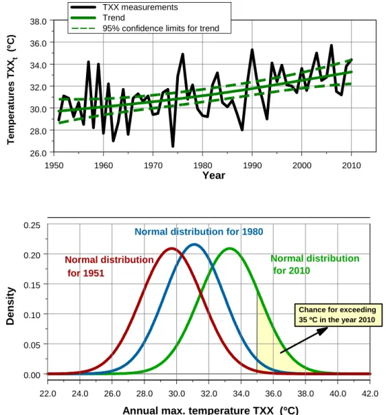
the Netherlands we constructed a time series for this indi-cator over the period 1901–2010 (station De Bilt). Homo-geneity tests showed a large discontinuity in 1950, the year where the type of temperature screen changed. Therefore, we decided to limit analyses to the period 1951–2010. Other ho-mogeneity tests were satisfactory (Visser, 2007). The TXXt

series is shown in Fig. 1.

The upper panel shows the data along with an Integrated Random Walk (IRW) trend model and 95 % confidence lim-its (Visser, 2004; Visser and Petersen, 2009). Tests showed the residuals (or in Kalman filter terms: innovations or one-step-ahead prediction errors) to be normally distributed. These normal distributions are shown in the lower panel for the years 1951, 1980 and 2010. The panel shows how chances (p35_t ) of crossing a certain threshold, here 35◦C, are changing for these three distributions (the yellow areas). For this example we find p₁₉₅₁35 =0.002, p35₁₉₈₀=0.02 and

p₂₀₁₀35 =0.18. Average return periods are gained by taking the inverse ofp_t35, yielding return periodsR_t35of once in 420, 62 and 5.6 yr, respectively. For the calculation of annual 20-yr return periods (TXX20_t )we choose the yellow area such that it covers 5 % of right-hand tail of the normal distributions, for all timest. We find the temperature thresholds 32.8, 34.1 and 36.4◦C, respectively (cf. Fig. 6).

2.4 Comparing PDFs

(5)

0.00 0.05 0.10 0.15 0.20 0.25

D

e

n

s

it

y

Normal distribution for 2010

22.0 24.0 26.0 28.0 30.0 32.0 34.0 36.0 38.0 40.0 42.0

Annual max. temperature TXX (°°°°C)

Chance for exceeding 35 °°°°C in the year 2010 Normal distribution

for 1951

Normal distribution for 1980

1950 1960 1970 1980 1990 2000 2010

26.0 28.0 30.0 32.0 34.0 36.0 38.0

Year

TXX measurements Trend

95% confidence limits for trend

T

e

m

p

e

ra

tu

re

s

T

X

Xt

(

°°°°

C

)

Fig. 1.Example of an extreme weather indicator, the TXXtseries for station De Bilt in the Netherlands. The upper panel shows the annual

data, along with an IRW trend fit (µt)and 95 % confidence limits. The lower panel shows three normal distributions corresponding to the

years 1951, 1980 and 2010. The yellow area illustrates the chance of crossing the 35◦C threshold. Clearly, the area for the years 1951 and

1980 is much smaller, a phenomenon first shown by Mearns et al. (1984) and Wigley (1985). A return period is calculated as the inverse of these chances. For each of the three normal distributions one could calculate the temperature which is exceeded once in x years, the x-year return periods. For statistical details see Von Storch and Zwiers (1999, Ch. 2). Chances and return periods are further illustrated in Fig. 6.

2.5 Software

Standard statistical techniques mentioned in this Section are available in software packages such as SPSS, S-PLUS, SAS or STATA. These packages also contain a wide range of trend models (OLS straight lines and polynomials, ARIMA models, robust trend models (MM or LTS), and a range of smoothing filters (splines, Kernel smoothers, LOESS smoothers, Supersmoothers).

For the estimation of GEV models and POT-GPD distri-butions (stationary or non-stationary) we refer to Stephen-son and Gilleland (2006) and Gilleland and Katz (2011). On their website a wide range of software is given, based

on extreme value theory (EVT): http://www.ral.ucar.edu/

\simericg/softextreme.php. For a software package based on the book of Coles (2001) the reader to the extRemes soft-ware, written in R: http://cran.r-project.org/web/packages/ extRemes/extRemes.pdf.

(6)

2.6 Methods in the literature

In this Section, we will give a concise overview of the recent literature on extremes and disasters. In doing so, we have categorized the literature for the stationarity assumptions that researchers have made. Besides stationarity and non-stationarity we will give examples for block-non-stationarity, that is a period or “block” of a certain length, typically between 20 to 30 yr, where climate is assumed to be stationary. 2.6.1 Assuming a stationary climate

Non-statistical approaches

Extreme events or disasters can be analysed without as-suming statistical properties. The method employed is simply by enumerating a number of record-breaking val-ues. These records can be discussed with respect to their spreading over time. If x of the highest values oc-curred in the past decade, this might give an indication of a shifting climate. The method of enumeration is of-ten applied in communication to the media. An example is the annually recurring discussions on the extremity of global mean temperatures. For example, see the NOAA and NASA GISS websites http://www.noaanews.noaa.gov/ stories2011/20110112 globalstats.html and http://www.giss. nasa.gov/research/news/20110113/, discussing the extremity of the 2010 value.

In the peer-reviewed literature enumeration is found only incidentally. For instance, Prior and Kendon (2011) stud-ied the UK winter of 2009/2010 in relation to the severity of winters over the last 100 yr. They give an overview of coldness rankings for monthly and seasonal average temper-atures, as well as rankings for the number of days with snow. Furthermore, Battipaglia et al. (2010) study temperature ex-tremes in Central Europe reconstructed from tree-ring den-sity measurements and documentary evidence. Their tables and graphs show a list of warm and cold summers over the past five centuries.

In the grey literature (reports) many examples of enumer-ation can be found. Buisman (2011) gives a detailed descrip-tion of weather extremes and disasters, for a large part based on documentary information in the area of the Netherlands. His enumeration covers the period from the Middle Ages up to the present. Enumerations of disasters in recent decades are found in, e.g. WHO (2011) and Munich Re (2011).

Statistical approach assuming no specific PDF

Zorita et al. (2008) consider the likelihood that the ob-served recent clustering of warm record-breaking mean temperatures at global, regional and local scales may oc-cur by chance in a stationary climate. They conclude this probability to be very low (under two different hypotheses).

Assuming GEV distributions

Wehner (2010) fits GEV distributions to pre-industrial con-trol runs from 15 climate models in the CMIP3 dataset. These control runs are assumed to be stationary; 20-yr return periods are estimated for annual maximum daily mean sur-face air temperatures along with uncertainties in these return periods. Min et al. (2011) also estimate the GEV distribu-tion. They analyse 49-yr time series of the largest one-day and five-day precipitation accumulations annually (RX1Dt

and RX5Dt). Afterwards, these distributions are used to

transform precipitation data to a “probability-based index” (PI), yielding a new 49-yr time series with values between 0 and 1. Time-dependent behaviour of the PIt series is shown

by estimating trends (their Fig. 1).

Assuming GDP distributions (POT approach)

Della-Marta et al. (2009) apply the POT approach in com-bination with the generalized Pareto distribution (GDP) and declustering. They apply this approach to extreme wind speed indices (EWIs). The GDP parameters are regarded to be time-independent.

Assuming normal distributions

Sch¨ar et al. (2004) estimate a normal distribution through monthly and summer temperatures in Switzerland, 1864– 2003, to characterise the 2003 European heat wave (their Figs. 1 and 3). Barriopedro et al. (2011) estimate a normal distribution for European summer temperatures for 1500– 2010 (see their Fig. 2). The five coldest and highest values are highlighted. The 2010 summer temperature appears to be the highest by far.

2.6.2 Assuming a block-stationary climate

Assuming no specific PDF shape

Alexander et al. (2006) analyse changes in PDF shapes with-out specifying the shape itself. In their Fig. 8 the sam-ple period (1901–2003) is split-up into three block periods and PDF shapes are discussed in a qualitative way. In their Figs. 9, 10 and 11 two block periods have been chosen. Brown et al. (2010) analyse temporal changes in PDFs in their Figs. 5 and 6. Data are seasonal minimum and max-imum temperatures over the period 1893–2005, taken from northeastern US stations. The block size is around 28 yr. No specific PDF shape is assumed in their analyses.

(7)

model simulations. For that purpose they assume climate to be stationary over 20-yr periods. For selected blocks GEV distributions are estimated and 20-yr return periods are cal-culated. They argue that longer return periods (≥50 yr) are less advisable given the short block length of 20 yr. Bar-riopedro et al. (2011) analyse multi-model projections of fu-ture mega-heatwaves (their Fig. 4). To this end they choose blocks of 30 yr and base their return-period calculations on these 30-yr blocks. Uncertainties in return periods are gained through 1000 times resampling of block data. Zwiers et al. (2011) choose 10-yr blocks for the location parameter of the GEV distribution. The other two GEV parameters are kept constant in their approach.

Assuming normal distributions

Beniston and Diaz (2004) use a block length of 30 yr to anal-yse the rarity of the 2003 heat wave in Europe. They esti-mate a normal distribution through mean summer maximum temperature data at Basel, Switzerland, for the 1961–1990 period. They argue that what may be regarded as an extreme beyond the 90th percentile under current (= stationary) cli-mate, becomes the median by the second half of the 21st century. Their results are repeated in Trenberth and Jones (2007, p. 312 – Fig. 2, lower panel).

2.6.3 Assuming a non-stationary climate

Tr¨omel and Sch¨onwiese (2005, 2007) analyse monthly to-tal precipitation data from a German station network of 132 time series, covering the period 1901–2000. They use a de-composition technique which results in estimations of Gum-bel distributions with a time-dependent location and scale parameter. Kharin and Zwiers (2005) estimate extremes in transient climate-change simulations. Their sample period is 1990–2100. They assume annual extremes of temperature and precipitation to be distributed according to a GEV distri-bution with all three parameters time-varying (linear trends). In doing so, their GEV model has six unknown parame-ters to be estimated. Brown et al. (2008) essentially follow the same approach for extreme daily temperatures over the period 1950–2004.

Fowler et al. (2010) estimate GEV distributions with lin-ear changing location parameters and apply this technique to UK extreme precipitation simulations over the period 2000– 2080. Their approach deviates from that of Kharim and Zwiers (2005) and Brown et al. (2008) in that they do not assume this approach to be the only approach possible. They estimate eight different modelling approaches and evaluate the best fitting model using Akaike’s AIC criterion. Hanel et al. (2009) apply GEV distributions where all three parame-ters are time-varying. Furthermore, the GEV location param-eter may vary over the region. This non-stationary model has

been applied to the 1-day summer and 5-day winter precip-itation maxima in the river Rhine basin, in a model simula-tion for the period 1950–2099. A similar approach has been followed by Hanel and Buishand (2011).

Assuming GPD distributions

Katz et al. (2002) assumes a general Pareto distribution for US flood damages where a linear trend is assumed in the log-transformed scale parameter (their Fig. 5). Parey et al. (2007) assume a POT model with time-varying parame-ters and analyse 47 temperature stations in France over the 1950–2003 period. As in Fowler et al. (2010) they consider a suit of models such as situations where station data are as-sumed to be stationary versus those where they are asas-sumed to be non-stationary.

Coelho et al. (2008) apply a flexible generalized Pareto model that accounts for spatial and temporal variation in excess distributions. Non-stationarity is introduced by us-ing time-varyus-ing thresholds (local polynomial with a win-dow of 20 yr). Sugahara et al. (2009) apply the same ap-proach as Coelho et al. (2008), using large p quantiles of daily rainfall amounts. A sensitivity analysis was per-formed by estimating four different GPD models. Acero et al. (2011) use the POT-GDP approach where thresholds are made time-varying, allowing them to change linearly over time. An automatic declustering approach was used to select independent extreme events exceeding the threshold.

Assuming normal or log-normal distributions

Wigley (2009) analyses changes in return periods using OLS trend fitting plus a normal distribution for the residuals. He gives an example for monthly mean summer temperatures in England (the CET database). We come to this approach in more detail in Sect. 4.1. Visser and Petersen (2009) ap-ply a trend model from the group of structural time series models, the so-called Integrated Random Walk (IRW) model. This IRW model has the advantage of being flexible where the flexibility can be chosen by maximum likelihood opti-mization. The OLS straight line is a special case of the IRW model. They apply this trend model to an indicator for extreme cold conditions in the Netherlands for the pe-riod 1901–2008. Return pepe-riods are generated along with uncertainty information on temporal changes in these return periods (cf. the TXXtexample shown in the Figs. 1, 4 and 6).

Estimating trends only

(8)

Kendall’s tau-based slope estimator. Klein Tank et al. (2006) apply LOWESS smoothers in their Figs. 3, 4, 6 and 7. Re-sults using straight lines are also presented. Here, OLS fits are used where significance is tested using a Student’s t-test. Pielke (2006) shows several examples of trend estimation for disaster data. Both OLS straight lines are shown (after taking a log-transformation) and 11-yr centred moving averages.

3 Stationarity assumptions

3.1 Stationarity

We have seen in Sect. 2 that methods fall apart with respect to their assumption of stationarity (Sects. 2.6.1, 2.6.2 and 2.6.3). At first glance one may judge this choice as a matter of taste. As long as one makes his or her assumptions clear, all seems okay at this point. Of course, there is no problem as long as the processes underlying the data at hand are truly stationary, such as in the study of Wehner (2010) who esti-mates GEV distributions to pre-industrial control runs from 15 climate models, part of the CMIP3 dataset. The same holds for Villarini et al. (2011) who apply GEV distribu-tions for extreme flooding stadistribu-tions with stationary data over time only.

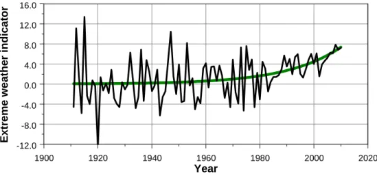
However, inferences might go wrong if data are assumed to be stationary when they are not. Figure 2 gives an illus-tration of this point by simulation. Suppose that a specific weather index shows an increasing trend pattern over time. However, the year-to-year variability slowly decreases over time (heteroscedastic residuals). Now, if we would assume these data to be stationary, we would conclude that the fre-quency of high extremes is decreasing over time. This con-clusion could be easily interpreted as an absence of climate change. However, the increasing trend in these data is tradictory to this conclusion. The example shows that con-clusions on the influence of climate change should not be done on the behaviour of extremes alone. Proper methods for stationary checks should be applied.

A second danger of assuming stationarity while data are in fact non-stationary, occurs if GEV distributions are applied. GEV distributions are very well suited to fit data which are stable at first and start to rise at the end. See the simula-tion example in Fig. 3, upper panel. This example is com-posed of an exponential curve where normally distributed noise is added. Now, if we regard this hundred-year long record as stationary and estimate for example the Gumbel distribution to these data, a perfect fit is found, as illustrated in the lower panel.

This result might seem surprising, but it is not. The resid-uals of the simulated series are normally distributed, hav-ing symmetric tails. Due to the higher values at the end of the series the right-hand tail of the distribution will become “thicker” than the tail of the normal distribution if we dis-card the non-stationarity at the end of the series. And this is exactly the shape of the right-hand tail of the Gumbel

distri-bution, and more generally the GEV distribution. In practice the GEV distribution will give a good fit in many such oc-casions since it hasthreefit parameters instead of the two of the Gumbel distribution.

Our conclusion is that care should be taken if climate is assumed to be stationary. If data are assumed to be stationary when they are not, inferences might become misleading.

Thus, proper testing for stationarity versus non-stationarity is a prerequisite. For examples of non-stationarity tests please refer to Feng et al. (2007), Diermanse et al. (2010), Fowler et al. (2010), Furi´o and Meneu (2011), Villarini et al. (2011) and Rea et al. (2011).

3.2 Block stationarity

As we have described in Sect. 2.6.2, a number of authors as-sume their data to be stationary over short periods of time, typically periods of 20 to 30 yr. Such assumptions are of-ten made in climatology and are clearly reflected in the definition of “climate” (IPCC, 2007, WG I, Annex I): Cli-mate in a narrow sense is usually defined as the average weather, or more rigorously, as the statistical description in terms of the mean and variability of relevant quanti-ties over a period of time ranging from months to

thou-sands or millions of years. The classical period for

av-eraging these variables is 30 yr, as defined by the World

Meteorological Organization [...](http:// www.ipcc.ch/ pdf/ assessment-report/ ar4/ syr/ ar4 syr appendix.pdf ).

Of course, if the extreme indicator at hand shows stable be-haviour over the block period chosen, the choice of stationar-ity is satisfactory. However, due to rapid climate change, the stationarity assumption may be invalid, even for very short periods. Young et al. (2011) give such examples for 23-yr extreme wind speed and wave height data. They find many significant rising trends (their Table 1 and Fig. 3).

Another example is the TXXt series shown in the upper

panel of Fig. 1. The Figure shows an almost linear increase of these annual maximum temperatures. To analyse the local behaviour of this trend more closely, we estimated the trend differences [µ2010–µt−1] and [µt–µt−1] along with 95 % confidence limits (statistical approach explained in Visser, 2004). See Fig. 4. The Figure shows that the trend value

µ2010 in the final year 2010 is significantly larger thanany trend value µs in the period 1951–2009 (α= 0.05). The

lower panel shows an even stronger result: all trend differ-ences [µt–µt−1] over the period 1967–2010 are significantly positive (α= 0.05).

(9)

1900 1920 1940 1960 1980 2000 2020

Year

-12.0 -8.0 -4.0 0.0 4.0 8.0 12.0 16.0

E

x

tr

e

m

e

w

e

a

th

e

r

in

d

ic

a

to

r

Fig. 2.Simulated extreme weather indicator for the sample period 1911–2010. The “measurements” are gained by choosing an exponential as a “trend” (green line) and adding a normally distributed white noise process to this trend. The variance of the noise is linearly decreasing over time.

4 Choice of probability distribution assumptions

4.1 PDF shapes: normal or GEV?

As described in Sect. 2.6, different types of probability dis-tributions have been applied to both stationary and non-stationary extreme indicator data. For example, Beniston and Diaz (2004) applied the normal distribution, Visser and Petersen (2009) applied the log-normal distribution, Tr¨omel and Sch¨onwiese (2006) applied the Gumbel distribution and Brown et al. (2008) applied the GEV distribution. This leads to the question of which distribution is preferable in which situation? Or would it be possible that different PDFs fit equally well to the same data? If the latter were true, it would still be worthwhile to choose the PDF with care if extrapo-lations are made far beyond the sample record length (re-turn periods of once in 500 to 1000 yr, as in Della-Marta et al. (2009) or Lucio et al. (2010)).

In this context, the comments of Cooley (2009) to an ar-ticle of Wigley (2009, reprinted from 1988) are relevant. Wigley estimated linear trends and normal distributions to monthly mean temperatures in England (the CET database, Parker and Horton, 2005). Cooley estimated GEV dis-tributions with time-varying parameters to annual maxima of daily maximum temperatures, also taken from the CET database. He finds a linear fit for the GEV location (mean) parameter, and constants for the variance and shape parame-ter. Cooley discusses the advantages of taking the GEV dis-tribution rather than the normal disdis-tribution. Who is right, or are both right?

We re-estimated the CET TXXt data3with the IRW trend

model (cf. Fig. 1), and checked the distribution of the resid-uals. The IRW flexibility is estimated by ML optimization and appears to be a straight line, mathematically equal to the OLS linear trend. The innovations (= one-step-ahead pre-diction errors) do not show obvious non-normal behaviour and we conclude that a straight line, along with normally distributed residuals, gives feasible results for these TXXt

data. Compared to the trend of Cooley, our trend appears to have a slightly steeper slope: 0.0155±0.005 (1-σ ) against their slope estimate 0.0142. This result implies that (i) more than one PDF may be applied to the same data and (ii) the choice of the PDF shape (slightly) influences the trend slope estimate (cf. the simulation example shown in Fig. 3).

4.2 Comparing four PDF shapes

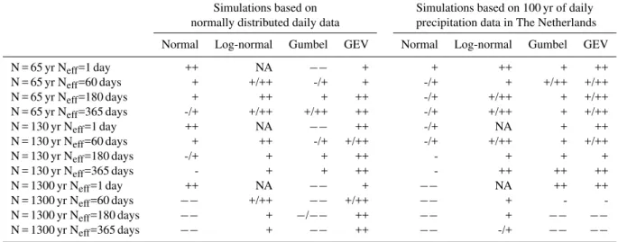
To get a better grip on this “PDF shape discussion” we have tested four PDF shapes frequently encountered in the litera-ture, on the same data. PDF shapes are (i) the normal distri-bution, (ii) the log-normal distridistri-bution, (iii) the Gumbel dis-tribution and (iv) the GEV disdis-tribution (of which the Gumbel distribution is a special case). For such a test, we performed two groups of simulations yielding a number of TXXt and

RX1Dt “look alikes”. We varied the time series length N

(65, 130 and 1300 yr) and the number of effective days Neff (1, 60, 180 and 365 days). The latter parameter mimics the effective number of independent daily data within a year for a certain weather variable. Details are given in Appendix A.

3_{The CET TXX}

t temperatures can most easily be downloaded

(10)

1900 1920 1940 1960 1980 2000 2020 Year

-4.0 0.0 4.0 8.0 12.0

E

x

tr

e

m

e

w

e

a

th

e

r

in

d

ic

a

to

r

0 5 10

0

.0

0

.0

5

0

.1

0

.1

5

Indicator

R

e

la

ti

v

e

F

re

q

u

e

n

c

y

Histogram of Observed Data with Fitted Extreme Value Distribution

Order Statistics for Indicator and

Extreme Value(location=0.3981642, scale=2.079251) Distribution

C

u

m

u

la

ti

v

e

P

ro

b

a

b

ili

ty

-2 0 2 4 6 8 10

0

.0

0

.2

0

.4

0

.6

0

.8

1

.0

Empirical CDF for Indicator (solid line) with Fitted Extreme Value CDF (dashed line)

Quantiles of Extreme Value(location = 0.3981642, scale = 2.079251)

Q

u

a

n

ti

le

s

o

f

In

d

ic

a

to

r

-2 0 2 4 6 8 10

-2

0

2

4

6

8

1

0

Quantile-Quantile Plot with 0-1 Line

Results of Kolmogorov-Smirnov GOF

Hypothesized

Distribution: Extreme Value Estimated Parameters: location = 0.3981642 scale = 2.079251 Data: Indicator in extreme

Sample Size: 100

Test Statistic: ks = 0.0542364 Test Statistic Parmeter: n = 100 P-value: 0.9302782

Results of Kolmogorov-Smirnov GOF Test for Indicator in extreme

Fig. 3.The upper panel shows a simulated extreme weather indicator over the sample period 1911–2010. The “measurements” are gained by choosing an exponential as a “trend” and adding normal distributed white noise to this trend (constant variance) . If it is assumed that

the measurements follow astationaryprocess, the data appear to follow an extreme value (Gumbel) distribution. This is shown in the lower

four panels which are generated by the S-PLUS Envstats module. Shown is the Kolmogorov-Smirnov test, where the data are compared to a

Gumbel distribution. The Gumbel distribution appears to fit very well (QQ-plot shows all data on the 0–1 line;pvalue of the KS test is 0.93).

An example from these simulations is given in Fig. 5. Here, we have plotted four PDFs for the same TXXt

simula-tion (Neff= 60 days; N = 130 yr). This simulation resembles the Wigley – Cooley case with daily CET temperatures since 1880. The four panels show the Kolmogorov-Smirnov good-ness of fit test, along with three graphic presentations (as in the lower panel of Fig. 3). The panels show that the only dis-tribution which fitsnotvery well, is the Gumbel distribution (right tail deviates in the QQ plot, panel lower left).

Although the simulation exercise described in Ap-pendix, is certainly not exhaustive, the following inferences can be made:

– both log-normal and GEV distributions fit very well for the vast majority of simulations, (both TXXt and

RX1Dt simulations). This result is in line with the

many examples of these PDFs in the literature, applied to real data.

– the Gumbel distribution fits only moderately to the TXXt simulations. Much better fits are found for data

which are skewed in nature, such as in case of the RX1Dt simulations. This result is in line with the

(11)

1950 1960 1970 1980 1990 2000 2010

Year

-2.0 0.0 2.0 4.0 6.0

µ µ µ µ 20

10

20

10

20

10

20

10

-µµµµ t

(

°°°°

C

)

Trend difference between 2010 and all preceeding years t Corresponding 95% confidence limits

1950 1960 1970 1980 1990 2000 2010

Year

-0.10 -0.05 0.00 0.05 0.10 0.15 0.20

µ µ µ µττττ

-µµµµ

t-1

(°°°°

C

)

Trend differences between consecutive years Corresponding 95% confidence limits

Fig. 4.Uncertainties for the IRW trend estimates shown in Fig. 1. The upper panel shows the trend difference [µ2010−µt] along with 95 %

confidence limits, the lower panel the trend differences [µt−µt−1] along with 95 % confidence limits.

– The normal distribution fits well for the TXXt

simu-lations as long as the number of years is rather small (sample periods shorter than∼130 yr). This result is in line with the Wigley – Cooley discussions for CET data since 1880. For skewed data, as in the second group of simulations, the normal distribution is not a good choice.

One might conclude from the inferences above that the GEV distribution would be the ideal PDF choice in gen-eral: (i) it fits in almost all cases and (ii) it has an interpre-tational background in relation to extremes. However, we note that the estimation of time-varying GEVs in combina-tion with linearity assumpcombina-tions on the three parameters, de-mands the estimation of six parameters (Kharin and Zwiers, 2005). And the linearity assumption for GEV parameters might be limiting in some cases. In contrast, the estimation of flexible trends and normal distributions (as in the TXXt

examples for CET and De Bilt) (i) does not fit for skewed data and (ii) lacks interpretation. However, it demands the estimation of only one parameter. Also uncertainty infor-mation on extremes is gained more easily (cf. Fig. 6). The same advantage is gained after taking logarithms of the indi-cator at hand, as in Visser and Petersen (2009 – their Fig. 5

and Appendix). The simulations in Appendix A show that log-normal distributions fit very well.

We found one example in the literature where different PDFs are analysed for the same data. Sobey (2005) analyses detrended high and low water levels according to four differ-ent PDF shapes: the Gumbel distribution, the Fr´echet distri-bution, the Weibull distribution and the log-normal tion (the first three distributions are part of the GEV distribu-tion). Furthermore, he gives a guidance for choosing the suit-able distribution for the data at hand. For both extreme high and extreme low water levels at San Francisco the log-normal distribution fits best to the data. He identifies the Gumbel and Weibull distribution as promising alternatives. His results are consistent with the findings from our simulation study above (although different in detail).

5 Uncertainty information

5.1 Available statistical techniques do not suffice in all cases

(12)

1.5 2.0 2.5 3.0 0 .0 0 .2 0 .4 0 .6 0 .8 1 .0 Max R e la ti v e F re q u e n c y

Histogram of Observed Data with Fitted Normal Distribution

Order Statistics for Max and Normal(mean=2.292642, sd=0.423567) Distribution

C u m u la ti v e P ro b a b il it y

1.5 2.0 2.5 3.0

0 .0 0 .2 0 .4 0 .6 0 .8 1 .0

Empirical CDF for Max (solid line) with Fitted Normal CDF (dashed line)

Quantiles of Normal(mean = 2.292642, sd = 0.423567)

Q u a n ti le s o f M a x

1.5 2.0 2.5 3.0

1 .5 2 .0 2 .5 3 .0 Quantile-Quantile Plot with 0-1 Line

Hypothesized

Distribution: Normal

Estimated Parameters: mean = 2.292642

sd = 0.423567

Data: Max in SimulationEVA

Sample Size: 130

Test Statistic: ks = 0.07038697

Test Statistic Parmeter: n = 130

P-value: 0.5400239

Results of Kolmogorov-Smirnov GOF Test for Max in SimulationEVA

Q

1.5 2.0 2.5 3.0

0 .0 0 .2 0 .4 0 .6 0 .8 1 .0 Max R e la ti v e F re q u e n c y

Histogram of Observed Data with Fitted Lognormal Distribution

Order Statistics for Max and Lognormal(meanlog=0.8124098, sdlog=0.1883455) Distribution

1.5 2.0 2.5 3.0

0 .0 0 .2 0 .4 0 .6 0 .8 1 .0

Empirical CDF for Max (solid line) with Fitted Lognormal CDF (dashed line)

Quantiles of Normal(mean = 0.8124098, sd = 0.1883455)

Q u a n ti le s o f L o g [M a x ]

0.2 0.4 0.6 0.8 1.0 1.2

0 .2 0 .4 0 .6 0 .8 1 .0 1 .2 Quantile-Quantile Plot with 0-1 Line

Hypothesized

Distribution: Lognormal

Estimated Parameters: meanlog = 0.8124098

sdlog = 0.1883455

Sample Size: 130

P-value: 0.9680406

04 he

5) 1.5 2.0 2.5 3.0

Histogram of Observed Data with Fitted Extreme Value Distribution

Order Statistics for Max and Extreme Value(location=2.086014, scale=0.3912738) Distribution

1.5 2.0 2.5 3.0

0 .0 0 .2 0 .4 0 .6 0 .8 1 .0

Empirical CDF for Max (solid line) with Fitted Extreme Value CDF (dashed line)

Quantiles of Extreme Value(location = 2.086014, scale = 0.3912738)

1.5 2.0 2.5 3.0 3.5 4.0

1 .5 2 .0 2 .5 3 .0 3 .5 4 .0 Quantile-Quantile Plot with 0-1 Line

Hypothesized

Distribution: Extreme Value

Estimated Parameters: location = 2.086014

scale = 0.3912738

Sample Size: 130

P-value: 0.7290757

an

1.5 2.0 2.5 3.0

Histogram of Observed Data with Fitted Generalized Extreme Value Distribution

Order Statistics for Max and

Generalized Extreme Value(location=2.136043, scale=0.4064589, shape=0.2400465

1.5 2.0 2.5 3.0

0 .0 0 .2 0 .4 0 .6 0 .8 1 .0

Empirical CDF for Max (solid line) with Fitted Generalized Extreme Value CDF (dashed

of Generalized Extreme Value(location = 2.136043, scale = 0.4064589, shape = 0.2400465)

1.5 2.0 2.5 3.0

1 .5 2 .0 2 .5 3 .0 Quantile-Quantile Plot

with 0-1 Line Results of Kolmogorov-Smirnov GOF

Hypothesized

Distribution: Generalized Extreme Value

Estimated Parameters: location = 2.136043

scale = 0.4064589 shape = 0.2400465

Sample Size: 130

P-value: 0.7902691

Fig. 5.Kolmogorov-Smirnov graphs and statistics for a simulation example shown in Table A1 of Appendix A (maximum of 60 effective data in a year and a sample length of 130 yr). All four PDFs have been computed to the same data. Upper left panel: normal distribution; upper right panel: log-normal distribution; lower left panel: Gumbel distribution; lower right panel: GEV distribution.

Panel on Climate Change (IPCC), there has been increased attention to dealing with uncertainties over the last decade or so (see e.g. Moss and Schneider, 2000; Petersen, 2000, 2012; IPCC, 2005; Risbey and Kandlikar, 2007; Swart et al., 2009; Hulme and Mahony, 2010; Mastrandrea et al., 2010).

We scanned the literature for their treatment of statisti-cal uncertainties. In doing so, we discerned three levels of statistical uncertainty information:

– Class 0: research giving no statistical uncertainty information.

– Class 1: research giving point-estimate uncertainty for extreme statistics. Here, we mean uncertainty statistics at one specific point in time, such as confidence limits for a return periodRt or confidence limits for a trend

estimateµt. An example for extremes has been given

in the three panels of Fig. 6. An example for trends has been given in Fig. 1, upper panel.

– Class 2: research giving uncertainty information both for point estimates and for differential estimates. Here, we mean “Class 1” uncertainty information along with uncertainty information on differential statistics such as the return-period differential [Rt –Rs], or trend

differ-entials [µt–µs] (times “t” and “s” lie in the sample

pe-riod with t>s).4 An example has been given in Fig. 4.

4_{We note that some researchers apply the Mann-Kendall test for}

(13)

1950 1960 1970 1980 1990 2000 2010

Year

0.0 0.1 0.2 0.3 0.4 0.5

C

h

a

n

c

e

x

c

e

d

in

g

3

5

°°°°

C Chance on exceedance

Corresponding 95% confidence limits

1950 1960 1970 1980 1990 2000 2010

Year

0 200 400 600

R

e

tu

rn

p

e

ri

o

d

(y

e

a

rs

)

Return period for exceedance of 35.0 C Corresponding 95% confidence limits

1950 1960 1970 1980 1990 2000 2010

Year

30.0 32.0 34.0 36.0 38.0

T

X

t

h

re

s

h

o

ld

(

°°°°

C

) Threshold for 20 year return period _{Corresponding 95% confidence limits}

Fig. 6. Three characterisations of extremes with uncertainties corresponding to the TXXt example from Fig. 1. The first panel shows the

annual chance of crossing the 35◦C threshold (p35_t ); the second panel shows the corresponding return period for crossing that threshold

(R35_t , expressed in years); the third panel shows the temperature threshold that will be exceeded once every 20 yr (TXX20_t , expressed in◦C).

In all three panels 95 % confidence limits are shown.

This graph shows the trend differentials [µ2010−µt]

and [µt−µt−1], along with 95 % confidence limits. With respect to return periods or the chance for

cross-ing pre-defined thresholdswe found only rarely examples of

“Class 0”. In most cases “Class 1” uncertainty information is given: Feng and Nadarajah (2007), Della-Marta et al. (2009), Fowler et al. (2010), Wehner (2010) and Lucio et al. (2010). However, we found that “Class 2” uncertainty information is lacking almost completely. The only example we found was in a previous paper of ours (Visser and Petersen, 2009). There, we give approximate uncertainty estimates for return period differentials in an Appendix.

As fortrends, we only rarely found examples of “Class 0” uncertainty. Examples lacking uncertainty information are mostly found in the estimation of trends in disaster data: al-though OLS linear trends have been applied (and, thus, un-certainty information is easily available), no unun-certainty in-formation is given in publications. Other examples are those where moving averages of other digital filters have been ap-plied. These trend models are not statistical in nature and, thus, do not give uncertainty information.

(14)

1980 1985 1990 1995 2000 2005 2010

Year 0

50 100 150 200 250

A

n

u

a

l

lo

s

e

s

(U

S

D

2

0

9

b

il

li

o

n

) Losses from global weather-related disasters

IRW trend

95% confindence limits trend

Fig. 7a. Economic losses due to weather-related disasters in the period 1980–2009. The data and trend in the upper panel are taken from Munich Re (2010a). The trend has been estimated by the OLS straight line fit after taking logarithms. The lower panel shows the IRW trend fit on logarithms of the same data. Flexibility of the trend has been optimized by ML estimation (Visser, 2004).

Tank and K¨onnen (2003), Klein Tank et al. (2006), Alexan-der et al. (2006), Brown et al. (2010), Min et al. (2011) and Charpentier (2011). Brown et al. (2008) give full sta-tistical uncertainty information for the time-varying location parameter of the GEV distribution. Trends from the class of structural time series models (STMs), as shown here in Figs. 1 and 4, give a generalization of the OLS linear trend: they also give full statistical uncertainty information (Visser, 2004; Visser et al., 2010).

(15)

1950 1955 1960 1965 1970 1975 1980 1985 1990 1995 2000 2005 2010

Year

0 4 8 12 16

N

u

m

b

e

r

o

f

d

is

a

s

te

rs

Number of great natural disasters IRW trend

95% confindence limits trend

Fig. 7b.The upper panel shows the annual number of great natural disasters. Source of data is the website of Munich Re. The lower panel

shows an IRW trend, fit on logarithms of the same annual data (i.e. yt= log(xt + 1)). Flexibility of the trend has been optimized by ML

estimation. Details of the IRW trend fit are given by Visser (2004). Source upper graph: Munich Re (2010b), p. 37 and their website.

5.2 Best modelling practices and uncertainty

As described at the end of Sect. 2.2, some authors have cho-sen to apply more than one trend model to analyse their data. This type of sensitivity analysis does not evaluate uncertain-ties in estimators only, but also tries to find the influence of under-lying model assumptions – thus, often moving beyond

(16)

Fig. 8.Example of coupling climate change to one particular disaster: the 2010 flooding in Pakistan. Text taken from the Scientific American website: http://www.scientificamerican.com/article.cfm?id=is-the-flooding-in-pakist.

Carlo experiments where three ways of estimating linear trends have been evaluated (OLS linear trend, Kendall tau-based method and time-varying GEV distributions). In fact, the evaluation of different trend models, and corresponding uncertainty inferences, is a way of evaluatingstructural un-certainty, i.e. evaluating the potential influence of specific model assumptions.

An illustration of the importance of considering more than one trend model, is given in Fig. 7a. The upper panel shows the economic losses due to global weather-related disasters, as published by Munich Re (2010a). The trend is estimated by fitting the OLS linear trend model, after taking logarithms of the event data. The result is an exponential increasing trend. If an IRW trend is estimated, where the flexibility is optimized by ML (Visser, 2004), a different trend pat-tern arises (lower panel): an increase up to 1995 and a stabi-lization afterwards. The trend value in 2009 is significantly higher than trend values before 1987 (tested for α= 0.05, graph not shown here). A comparable example is given in Fig. 7b. The upper panel shows the number of great natural disasters, as published by Munich Re (2010b) and reprinted in Pielke (2010, p. 167). Again, the result is an exponential increasing trend. If an IRW trend is estimated, a different trend pattern arises (lower panel): an increase up to 1992 and a decrease afterwards. The trend value in 2010 is not

sig-nificantly higher than the trend values before 1980 (tested for α=0.05,graph not shown here). These two examples illustrate that the interpretation of trend patterns in extreme indicators might be influenced by the trend method chosen.

Another approach to assess structural uncertainty is the evaluation of the stationarity/non-stationarity of the data at hand (cf. discussion in Sect. 3). Examples are:

– Feng and Nadarajah (2007) estimate both stationary and non-stationary GEVs, and calculate return periods for both approaches.

– Fowler et al. (2010) evaluate 8 GEV models, both sta-tionary and non-stasta-tionary. For choosing the most ap-propriate model they use the AIC criterion.

We also found other sensitivity approaches which could be categorized under the term “best modelling practices”. In the field of future extremes it might be of importance to evalu-ate extreme statistics on the basis of more than one GCM or RCM. Examples are:

(17)

– Wehner (2010 – Fig. 1) calculates the inter-model un-certainty for return periods, based on daily data from 15 different CMIP3 models.

– Barriopedro et al. (2011 – Figs. 4 and S12) evaluate return periods for mega-heatwaves on the basis of 11 RCMs and one reanalysis run.

A second sensitivity approach deals with the sensitivity of trend estimates and corresponding uncertainties in relation to

thesample period length. Examples are:

– Moberg and Jones (2005 – Table 3) show significant trends for four periods: 1901–1999, 1921–1999, 1901– 1950 and 1946–1999.

– Klein Tank et al. (2006 – Table 2) show trend decadal in-crements with uncertainties for the periods 1961–2000 and 1901–2000.

We note that an analogous sensitivity example for linear trends has been given by Trenberth and Jones (2007 – FAQ 3.1, Fig. 1) for global mean temperatures. A variation is given by Young et al. (2011, Table S1). They present five different significance tests for their trends.

Finally, as described in Sect. 4.2, Sobey (2005) analyses detrended high and low water levels according to four differ-ent PDF shapes. From his analysis he gives a guidance for choosing the suitable distribution for the data at hand.

In our judgment, some form of sensitivity analysis is im-portant to assess the reliability of results. This conclusion of course pertains more generally to environmental research.

6 Coupling extremes or disasters to climate change

There are several ways to couple trends in extremes or dis-aster to (anthropogenic) climate change (see, e.g. Hegerl and Zwiers, 2007; Zwiers et al., 2011; Min et al., 2011 for spatio-temporal approaches). One has to be careful, however, in coupling individual extremes to climate change. In fact, sta-tistical inferences are about chances forgroupsof events and not aboutindividualevents.

Even though most publications do not strictly couple sin-gle extremes to climate change, that is, with 100 % cer-tainty, many are suggestive about the connection while they focus actually on the changed chances. A recent exam-ple on flooding is Pall et al. (2011) and an examexam-ple of suggestive information on the Pakistan floodings in 2010 is given in Fig. 8. An earlier example is constituted by publications on the 2003 heatwave in Europe. Schier-meier (2011) chooses as subtitle: can violent hurricanes, floods and droughts be pinned on climate change?

Scien-tist are beginning to say yes. For a recent discussion on

In-ternet, please refer to http://e360.yale.edu/feature/forum is extreme weather linked to global warming/2411/.

PBL (2010) has analysed the presenting of this 2003 heat wave as a consequence of climate change in IPCC (2007). The Working Group II Summary for Policymakers states, for Europe, on page 14: “For the first time, wide-ranging impacts of changes in current climate have been docu-mented: retreating glaciers, longer growing seasons, shift of species ranges, and health impacts due to a heat wave of unprecedented magnitude. The observed changes described above are consistent with those projected for future climate

change.”This text, as well as its counterparts in Table TS4.2

of the Technical Summary (p. 51) and in the Executive Sum-mary (p. 543), present the health impacts from the 2003 heat wave as an example of “wide-ranging impact of changes in current climate”. Thus, the text implicitly suggests that the 2003 heat wave is the result of recent climate change.

However, one can never attribute a specific extreme weather event of the past – such as that particular heat wave – to changes in current climate. In fact, we agree with Sch¨ar and Jendritzky (2004) who stated the following:“The Euro-pean heatwave of 2003: was it merely a rare meteorological event or a first glimpse of climate change to come? Probably

both.” Stott et al. (2004) come to a comparable conclusion:

“It is an ill-posed question whether the 2003 heatwave was

caused, in a simple deterministic sense, by a modification of the external influence on climate – for example, increasing concentration of greenhouse gases in the atmosphere – be-cause almost any such weather event might have occurred

by chance in an unmodified climate.” Finally, IPCC-SREX

(2011, p. 6) concludes that “the attribution of single extreme

events to anthropogenic climate change is challenging”.

7 Conclusions

In this article, we have given a concise overview of methods applied in the peer-review literature to make inferences on extreme indicators. Furthermore, we have evaluated these methods for specific choices that researchers have made. These choices are (i) the choice of a specific type of sta-tionarity, (ii) the choice for a specific PDF shape of the data (or residuals) at hand, (iii) the treatment of uncertainties and (iv) the coupling of extremes or disasters to climate change. We draw the following conclusions:

– In making a choice for treating data as stationary or non-stationary, good testing is essential. Inferences on extremes may be wrong if data are assumed stationary while they are not (cf. Figs. 2 and 3). Some researchers choose block-stationarity (blocks of 20 to 30 yr). How-ever, climate may be non-stationary even for such short periods (cf. Figs. 1 and 4). Thus, such an assumption needs testing too.

(18)

Table A1.Judgments of distributional fits for (i) simulated meteorological data (cf. Fig. 5) and (ii) daily precipitation data in the Netherlands.

Meaning of codes:−−stands for a very bad fit;−stands for a bad fit; + stands for a good fit; ++ stands for a very good fit. These judgments

are based on visual inspection of the actual fits and onpvalues of the Kolmogorov-Smirnov goodness of fit tests. All judgments are based

on three repeated simulations (using different seeds in random number generation). Data in black are for 65 yr of simulation, in blue for 130 and in green for 1300 yr of simulation.

Simulations based on Simulations based on 100 yr of daily

normally distributed daily data precipitation data in The Netherlands

Normal Log-normal Gumbel GEV Normal Log-normal Gumbel GEV

N = 65 yr Neff=1 day ++ NA −− + + ++ + ++

N = 65 yr Neff=60 days + +/++ -/+ + -/+ + +/++ +/++

N = 65 yr Neff=180 days + ++ + ++ -/+ +/++ + +/++

N = 65 yr Neff=365 days -/+ +/++ +/++ ++ -/+ +/++ + +/++

N = 130 yr N_eff=1 day ++ NA −− ++ -/+ NA + ++

N = 130 yr Neff=60 days + ++ -/+ +/++ -/+ +/++ + +/++

N = 130 yr Neff=180 days -/+ + + ++ - + + +

N = 130 yr Neff=365 days - + + ++ - ++ ++ ++

N = 1300 yr Neff=1 day ++ NA −− + −− NA ++ ++

N = 1300 yr Neff=60 days −− +/++ −− +/++ −− + -

-N = 1300 yr -Neff=180 days −− + −/−− ++ −− + −− −−

N = 1300 yr N_eff=365 days −− + −− ++ −− -/+ −− −−

Cooley – Wigley example, and Fig. 5). From a simula-tion study we conclude that both the GEV and the log-normal PDF fit very well to a variety of indicators (both symmetric and skewed data/residuals). The normal PDF performs well for data which are (i) essentially symmet-rical in nature (such as extremes for temperature data) and (ii) have relatively short sample periods (∼130 yr). The Gumbel PDF fits well for data which are skewed in nature (such as extreme indicators for precipitation). For symmetrical situations the Gumbel PDF does not perform very well.

– Statistical techniques are not available for all cases of interest. We found that theory is lacking for uncertain-ties for differential statistics of return periods, i.e. uncer-tainties for a particular difference [Rt–Rs]. For trends

these statistics are available as long as OLS trends or structural time series models (STMs) are chosen (cf. Figs. 1 and 4).

– It is advised to test conclusions on extremes with respect to assumptions underlying the modelling approach cho-sen (structural uncertainty). Examples are given for (i) the application of different trend models to the same data, (ii) stationary versus non-stationary GEV mod-els, (iii) evaluation of extremes for a suite of GCMs or RCMS to evaluate statistics in the future, and (iv) the role of the sample period length. An example has been given where the choice of a specific trend model influences the inferences made (Fig. 7).

– The coupling of extremes to climate change should be performed by spatio-temporal detection methods.

How-ever, in the communication of extremes to the media it occurs that researchers couple one specific exceptional extreme event or disaster to climate change. This (sug-gestive) coupling should be avoided (Fig. 8). Statisti-cal inferences are always directed to chances forgroups

of data. They do not apply toonespecific occurrence within that group.

Appendix A

Simulation and PDF shapes

As described in Sect. 4.2, we have tested four PDF shapes frequently encountered in the literature, on the same data. PDF shapes are: the normal, the log-normal, the Gumbel and the GEV distribution (of which the Gumbel distribu-tion is a special case). For such a test, we performed two groups of simulations, one yielding TXXt “look alikes” and

one yielding RX1Dt “look alikes”. The first set is totally

based on random drawings from a normal distribution for daily values; the second set is based on real daily precipi-tation totals over the period 1906–2005 (De Bilt, the Nether-lands). We varied the time series length N (65, 130 and 1300 yr) and the number of effective days Neff(1, 60, 180 and 365 days). The latter parameter mimics the effective number of independent daily data within a year for a certain weather variable. The judgment of distributional fit has been done with two criteria: visual inspection of the QQ plot and the

pvalue from the Kolmogorov-Smirnov goodness of fit test

(p <0.05: bad result;p >0.80: very good result). See Fig. 5