Ailamazyan Program Systems Institute
Fifth International Valentin Turchin
Workshop on Metacomputation
Proceedings
Pereslavl-Zalessky, Russia, June 27 July 1, 2016
Pereslavl-Zalessky
ÁÁÊ 22.18 Ï-99
Fifth International Valentin Turchin Workshop on Metacomputation // Proceedings of the Fifth International Valentin Turchin Workshop on Meta- computation. Pereslavl-Zalessky, Russia, June 27 – July 1, 2016 / Edited by A. V. Klimov and S. A. Romamenko. — Pereslavl Zalessky: Publishing House
“University of Pereslavl”, 2016,184p. — ISBN 978-5-901795-33-0
Ïÿòûé ìåæäóíàðîäíûé ñåìèíàð ïî ìåòàâû÷èñëåíèÿì èìåíè
Â. Ô. Òóð÷èíà // Ñáîðíèê òðóäîâ Ïÿòîãî ìåæäóíàðîäíîãî ñåìèíàðà ïî ìåòàâû÷èñëåíèÿì èìåíè Â. Ô. Òóð÷èíà, ã. Ïåðåñëàâëü-Çàëåññêèé, 27 èþíÿ 1 èþëÿ 2016 ã. / Ïîä ðåäàêöèåé À. Â. Êëèìîâà è Ñ. À. Ðîìàíåíêî. Ïåðåñëàâëü- Çàëåññêèé: Èçäàòåëüñòâî ¾Óíèâåðñèòåò ãîðîäà Ïåðåñëàâëÿ¿, 2016, 184 ñ.
ISBN 978-5-901795-33-0
c 2016 Ailamazyan Program Systems Institute of RAS
Èíñòèòóò ïðîãðàììíûõ ñèñòåì èìåíè À. Ê. Àéëàìàçÿíà ÐÀÍ, 2016
ISBN 978-5-901795-33-0
(1931–2010)
The Fifth International Valentin Turchin Workshop on Metacomputation, META 2016, was held on June 27 – July 1, 2016 in Pereslavl-Zalessky. It be- longs to a series of workshops organized biannually by Ailamazyan Program Systems Institute of Russian Academy of Sciences and Ailamazyan University of Pereslavl.
The workshops are devoted to the memory of Valentin Turchin, a founder ofmetacomputation, the area of computer science dealing with manipulation of programs as data objects, various program analysis and transformation tech- niques.
The topics of interest of the workshops include supercompilation, partial eval- uation, distillation, mixed computation, generalized partial computation, slicing, verification, mathematical problems related to these topics, their applications, as well as cross-fertilization with other modern research and development direc- tions.
Traditionally each of the workshops starts with a Valentin Turchin memorial session, in which talks about his personality and scientific and philosophical legacy are given.
The papers in these proceedings belong to the following topics.
Valentin Turchin memorial
– Robert Gl¨uck, Andrei Klimov:Introduction to Valentin Turchin’s Cybernetic Foundation of Mathematics
Invited Speaker Neil D. Jones
– Neil D. Jones:On Programming and Biomolecular Computation
– Daniil Berezun and Neil D. Jones:Working Notes: Compiling ULC to Lower- level Code by Game Semantics and Partial Evaluations
Partial evalatuation
– Robert Gl¨uck:Preliminary Report on Polynomial-Time Program Staging by Partial Evaluation
Program slicing
– Husni Khanfar and Bj¨orn Lisper:Enhanced PCB-Based Slicing Distillation
– Venkatesh Kannan and G. W. Hamilton:Distilling New Data Types
– Andrew Mironov:On a Method of Verification of Functional Programs Proving Program Equivalence
– Sergei Grechanik:Towards Unification of Supercompilation and Equality Sat- uration
– Dimitur Krustev:Simple Programs on Binary Trees – Testing and Decidable Equivalence
Supercompilation
– Dimitur Krustev: A Supercompiler Assisting Its Own Formal Verification – Robert Gl¨uck, Andrei Klimov, and Antonina Nepeivoda: Non-Linear Con-
figurations for Superlinear Speedup by Supercompilation
– Antonina Nepeivoda: Complexity of Turchin’s Relation for Call-by-Name Computations
Derivation of parallel programs
– Arkady Klimov:Derivation of Parallel Programs of Recursive Doubling Type by Supercompilation with Neighborhood Embedding
Algorithms
– Nikolay Shilov: Algorithm Design Patterns: Programming Theory Perspec- tive
The files of the papers and presentations of this and the previous workshops as well as other information can be found at the META sites:
– META 2008:http://meta2008.pereslavl.ru/
– META 2010:http://meta2010.pereslavl.ru/
– META 2012:http://meta2012.pereslavl.ru/
– META 2014:http://meta2014.pereslavl.ru/
– META 2016:http://meta2016.pereslavl.ru/
May 2016 Andrei Klimov
Sergei Romanenko
Workshop Chair
Sergei Abramov, Ailamazyan Program Systems Institute of RAS, Russia
Program Committee Chairs
Andrei Klimov, Keldysh Institute of Applied Mathematics of RAS, Russia Sergei Romanenko, Keldysh Institute of Applied Mathematics of RAS, Russia
Program Committee
Robert Gl¨uck, University of Copenhagen, Denmark
Geoff Hamilton, Dublin City University, Republic of Ireland Dimitur Krustev, IGE+XAO Balkan, Bulgaria
Alexei Lisitsa, Liverpool University, United Kingdom Neil Mitchell, Standard Charted, United Kingdom
Antonina Nepeivoda, Ailamazyan Program Systems Institute of RAS, Russia Peter Sestoft, IT University of Copenhagen, Denmark
Artem Shvorin, Ailamazyan Program Systems Institute of RAS, Russia Morten Sørensen, Formalit, Denmark
Invited Speaker
Neil D. Jones, Professor Emeritus of the University of Copenhagen, Denmark
Sponsoring Organizations
Federal Agency for Scientific Organizations (FASO Russia) Russian Academy of Sciences
Russian Foundation for Basic Research (grant 16-07-20527-ã)
Working Notes: Compiling ULC to Lower-level Code by Game
Semantics and Partial Evaluations . . . 11 Daniil Berezun and Neil D. Jones
Preliminary Report on Polynomial-Time Program Staging by Partial
Evaluation . . . 24 Robert Gl¨uck
Introduction to Valentin Turchin’s Cybernetic Foundation of Mathematics 26 Robert Gl¨uck, Andrei Klimov
Non-Linear Configurations for Superlinear Speedup by Supercompilation. 32 Robert Gl¨uck, Andrei Klimov, and Antonina Nepeivoda
Towards Unification of Supercompilation and Equality Saturation. . . 52 Sergei Grechanik
On Programming and Biomolecular Computation. . . 56 Neil D. Jones
Distilling New Data Types . . . 58 Venkatesh Kannan and G. W. Hamilton
Enhanced PCB-Based Slicing. . . 71 Husni Khanfar and Bj¨orn Lisper
Derivation of Parallel Programs of Recursive Doubling Type by
Supercompilation with Neighborhood Embedding . . . 92 Arkady Klimov
A Supercompiler Assisting Its Own Formal Verification . . . 105 Dimitur Krustev
Simple Programs on Binary Trees – Testing and Decidable Equivalence. . 126 Dimitur Krustev
On a Method of Verification of Functional Programs. . . 139 Andrew Mironov
Complexity of Turchin’s Relation for Call-by-Name Computations. . . 159 Antonina Nepeivoda
Algorithm Design Patterns: Programming Theory Perspective . . . 170 Nikolay Shilov
Code by Game Semantics and Partial Evaluation
Daniil Berezun1and Neil D. Jones2
1 JetBrains and St. Petersburg State University (Russia)
2 DIKU, University of Copenhagen (Denmark)
Abstract. What:Any expressionM in ULC (the untypedλ-calculus) can be compiled into a rather low-level language we call LLL, whose pro- grams containnone of the traditional implementation devices for func- tional languages: environments, thunks, closures, etc. A compiled pro- gram is first-order functional and has a fixed set of working variables, whose number is independent ofM. The generated LLL code in effect traversesthe subexpressions ofM.
How: We apply the techniques ofgame semantics to the untypedλ- calculus, but take a more operational viewpoint that uses much less mathematical machinery than traditional presentations of game seman- tics. Further, the untyped lambda calculus ULC is compiled into LLL by partially evaluatinga traversal algorithm for ULC.
1 Context and contribution
Plotkin posed the problem of existence of a fully abstract semantics of PCF [17].
Game semantics provided the first solution [1–3, 9]. Subsequent papers devise fully abstract game semantics for a wide and interesting spectrum of program- ming languages, and further develop the field in several directions.
A surprising consequence: it is possible to build a lambda calculus interpreter withnone of the traditional implementation machinery:β-reduction; environ- ments binding variables to values; and “closures” and “thunks” for function calls and parameters. This new viewpoint on game semantics looks promising to see its operational consequences. Further, it may give a new line of attack on an old topic:semantics-directed compiler generation [10, 18].
Basis:Our starting point was Ong’s approach to normalisation of the simply typedλ-calculus(henceforth called STLC). Paper [16] adapts the game semantics framework to yield an STLC normalisation procedure (STNP for short) and its correctness proof using the traversal concept from [14, 15].
STNP can be seen as ininterpreter; it evaluates a givenλ-expressionM by managing a list of subexpressions ofM, some with a single back pointer. These notes extend the normalisation-by-traversals approach to theuntypedλ-calculus, giving a new algorithm called UNP, for Untyped Normalisation Procedure. UNP correctly evaluates any STLC expression sans types, so it properly extends STNP since ULC is Turing-complete while STLC is not.
Plan:in these notes we start by describing a weak normalisation procedure.
A traversal-based algorithm is developed in a systematic, semantics-directed way.
Next step: extend this to full normalisation and its correctness proof (details omitted from these notes). Finally, we explain briefly how partial evaluation can be used to implement ULC, compiling it to a low-level language.
2 Normalisation by traversal: an example
Perhaps surprisingly, the normal form of an STLCλ-expressionMmay be found by simply taking a walk over the subexpressions ofM. As seen in [14–16] there is no need forβ-reduction, nor for traditional implementation techniques such as environments, thunks, closures, etc. The “walk” is atraversal: a sequential visit to subexpressions ofM. (Some may be visited more than once, and some not at all.)
A classical example; multiplication of Church numerals3
mul=λm.λn.λs.λz.m(ns)z
A difference between reduction strategies: consider computing 3∗2 by evaluating mul3 2. Weak normalisation reducesmul3 2 only toλs.λz.3(2s)z but does no computation under the lambda. On the other hand strong normalisation reduces it further toλs.λz.s6z.
A variant is to use free variablesS, Zinstead of the bound variabless, z, and to usemul0=λm.λn.m(nS)Zinstead ofmul. Weak normalisation computes all the way:mul03 2 weakly reduces toS6Zas desired. More generally, the Church- Turing thesis holds: a functionf:Nn*Nis partial recursive (computable) iff there is aλ-expressionM such that for anyx1, . . . , xn, x∈N
f(x1, . . . , xn) =x ⇔ M(Sx1Z). . .(SxnZ) weakly reduces to SxZ The unique traversal of 3 (2S)Z visits subexpressions of Church numeral 3 once. However it visits 2 twice, since in generalx∗y is computed by adding y togetherxtimes. The weak normal form of 3 (2S)ZisS6Z: the core of Church numeral 6.
Figure 1 shows traversal of expression 2 (2S)Zin tree form4. The labels1:, 2:etc. are not part of theλ-expression; rather, they indicate the order in which subexpressions are traversed.
3 The Church numeral of natural number x is x = λs.λz.sxz. Here sx = s(s(. . . s(z). . .))withxoccurrences ofs, wheres represents “successor” andz represents “zero”.
4 Application operators @ihave been made exlicit, and indexed for ease of reference.
The two 2 subtrees are the “data’; their bound variables have been named apart to avoid confusion. The figure’s “program” is the top part ( S)Z.
Computation by traversal can be seen as a game
The traversal in Figure 1 is a game play between programλmλn.(m@ (n@S))@Z and the two data values (m, neach haveλ-expression 2 as value).
Informally: two program nodes are visited in steps 1, 2; then data 1’s leftmost branch is traversed from node λs1 until variable s1 is encountered at step 6.
Steps 7-12: data 2’s leftmost branch is traversed from nodeλs2 down to variable s2, after which the program node S is visited (intuitively, the first output is produced). Steps 13-15: the data 2 nodes @6ands2 are visited, and the program:
it produces the second outputS. Steps 16, 17:z2 is visited, control is finished (for now) in data 2, and control resumes in data 1.
Moving faster now: @4and the seconds1 are visited; data 2 is scanned for a second time; and the next two outputS’s are produced. Control finally returns toz1. After this, in step 30 the program produces the final outputZ.
DATA 1 z ⇓}| {
λs1 3:
? λz1 4:
?
@3
5:
? s1+ 6:
@4 : 17
? s1+ 18:
z1 : 29
⇐DATA 2 λs2
8, 20:
? λz2 9, 21:
?
@5
10, 22:
? s2+ 11, 23:
@6: 13, 25
? s2+ 14, 26:
z2 : 16, 28
PROGRAM⇒
1: @1
+ @
@ R
Z : 30 2: @2
HHHj 7, 19: @7
HHjS : 12, 15, 24, 27
Fig. 1.Syntax tree formul2 2S Z= 2(2S)Z. (Labels show traversal order.)
Which traversal? As yet this is only an “argument by example”; we have not yet explainedhow to chooseamong all possible walks through the nodes of 2(2S)Zto find the correct normal form.
3 Overview of three normalisation procedures
3.1 The STNP algorithm
The STNP algorithm in [16] is deterministic, defined by syntax-directed inference rules.
The algorithm is type-oriented even though the rules do not mention types:
it requires as first step the conversion from STLC toη-long form. Further, the statement of correctness involves types in “term-in-context” judgements Γ ` M:AwhereAis a type andΓ is a type environment.
The correctness proof involves types quite significantly, to construct program- dependent arenas, and as well a category whose objects are arenas and whose morphisms are innocent strategies over arenas.
3.2 Call-by-name weak normalisation
We develop a completely type-free normalisation procedure for ULC.5Semantics- based stepping stones: we start with an environment-based semantics that resem- bles traditional implementations of CBN (call-by-name) functional languages.
The approach differs from and is simpler than [13].
The second step is to enrich this by adding a “history” argument to the evaluation function. This records the “traversal until now”. The third step is to simplify the environment, replacing recursively-defined bindings by bindings from variables to positions in the history. The final step is to remove the envi- ronments altogether.
The result is a closure- and environment-free traversal-based semantics for weak normalisation.
3.3 The UNP algorithm
UNP yields full normal forms by “reduction under the lambda” usinghead linear reduction[7, 8]. The full UNP algorithm [4] currently exists in two forms:
– An implementation inhaskell; and
– A set of term rewriting rules. A formal correctness proof of UNP is nearing completion, using the theorem prover COQ [4].
5 Remark: evaluator nontermination is allowed on an expression with no weak normal form.
4 Weak CBN evaluation by traversals
We begin with a traditional environment-based call-by-name semantics: areduc- tion-freecommon basis for implementing a functional language. We then elimi- nate the environments by three transformation steps. The net effect is to replace the environments by traversals.
4.1 Weak evaluation using environments
The object of concern is a pair e:ρ, where e is a λ-expression and ρ is an environment6that binds some ofe’s free variables to pairse0:ρ0.
Evaluation judgements, metavariables and domains:
e:ρ⇓v Expressionein environmentρevaluates to valuev
v, e:ρ⇓v0 Valuevapplied to argumentein environmentρgives valuev0 ρ∈Env =V ar * Exp×Env
v∈V alue={e:ρ|edoes not have form (λx.e0)e1} Note: the environment domainEnv is defined recursively.
Determinism The main goal, given aλ-expressionM, is to find a valuevsuch thatM:[]⇓v(if it exists). The following rules may be thought of as analgorithm to evaluateM since they are are deterministic. Determinism follows since the rules aresingle-threaded: consider a goalleft⇓right. Ifleft has been computed butrightis still unknown, then at most one inference rule can be applied, so the final result value is uniquely defined (if it exists).
(Lam)
λx.e:ρ⇓λx.e:ρ (Freevar)xfree inM
x:ρ⇓x:[] (Boundvar) ρ(x)⇓v x:ρ⇓v Abstractions and free variables evaluate to themselves. A bound variablexis ac- cessed using call-by-name: the environment contains an unevaluated expression, which is evaluated when variablexis referenced.
(AP) e1:ρ⇓v1 v1, e2:ρ ⇓ v e1@e2:ρ ⇓ v
Rule (AP) first evaluates the operatore1in an applicatione1@e2. The valuev1 of operatore1determines whether rule (APλ) or (APλ) is applied next.
(APλ) e0=λx.e00 ρ00=ρ0[x7→e2:ρ] e00:ρ00⇓v e0:ρ0, e2:ρ ⇓ v
6 Call-by-name semantics: If ρcontains a bindingx 7→ e0:ρ0, then e0 is an as-yet- unevaluated expression andρ0is the environment that was current at the time when xwas bound toe0.
In rule (APλ) if the operator value is an abstractionλx.e00:ρ0thenρ0is extended by bindingxto the as-yet-unevaluated operande2(paired with its current en- vironmentρ). The body e00 is then evaluated in the extended ρ0 environment.
(APλ) e06=λx.e00 e2:ρ⇓e02:ρ02 fv(e0)∩dom(ρ02) =∅ e0:ρ0, e2:ρ ⇓ (e0@e02):ρ02
In rule (APλ) the operator value e0:ρ0 is a non-abstraction. The operande2 is evaluated. The resulting value is an application of operator valuee0 to operand value (as long as no free variables are captured).
Rule (APλ) yields a value containing an application. For the multiplication example, Rule (APλ) yields all of theSapplications in resultS@(S@(S@(S@Z))).
4.2 Environment semantics with traversal historyh
Determinism implies that there exists at most one sequence of visited subex- pressions for anye:ρ. We now extend the previous semantics to accumulate the history of the evaluation steps used to evaluatee:ρ.
These rules accumulate a listh= [e1:ρ1, . . . , , . . . , en:ρn] of all subexpressions ofλ-expressionMthat have been visited, together with their environments. Call such a partially completed traversal ahistory. A notation:
[e1:ρ1, . . . , en:ρn]•e:ρ= [e1:ρ1, . . . , en:ρn, e:ρ]
Metavariables, domains and evaluation judgements.
e:ρ, h⇓v Expressionein environmentρevaluates to valuev
v, e:ρ, h⇓v0 Valuevapplied to expressionein environmentρgives valuev0 ρ∈Env =V ar * Exp×Env
v∈V alue ={e:ρ, h|h∈History, e6= (λx.e0)e1} h∈History= (Exp×Env)∗
Judgements now have the form e:ρ, h ⇓ e0:ρ0, h0 where h is the history beforeevaluatinge, andh0is the historyafterevaluatinge. Correspondingly, we redefine a value to be of formv=e:ρ, hwhereeis not aβ-redex.
(Lam)
λx.e:ρ, h⇓λx.e:ρ, h•(λx.e:ρ) (Freevar) xfree inM
x:ρ, h ⇓ x:[], h•(x:[]) (Boundvar) ρ(x), h•(x:ρ) ⇓ v x:ρ, h ⇓ v
(AP) e1:ρ, h•(e1@e2, ρ)⇓ v1 v1, e2:ρ ⇓ v e1@e2:ρ, h ⇓ v
(APλ) e0=λx.e00 ρ00=ρ0[x7→e2:ρ] e00:ρ00, h0 ⇓ v e0:ρ0, h0, e2:ρ ⇓ v
(APλ) e06=λx.e00 e2:ρ, h0⇓e02:ρ02, h02 fv(e0)∩dom(ρ02) =∅ e0:ρ0, h0, e2:ρ⇓(e0@e02):ρ02, h02
Histories are accumulativeIt is easy to verify thathis a prefix ofh0whenever e:ρ, h⇓e0,:ρ0, h0.
4.3 Making environments nonrecursive
The presence of the history makes it possible to bind a variablexnot to a paire:ρ, but instead to the position of a prefix of historyh. Thusρ∈Env=V ar→N.
Domains and evaluation judgement:
e:ρ, h⇓v Expressionein environmentρevaluates to valuev
v, e:ρ, h⇓v0 Valuevapplied to argumentein environmentρgives valuev0 ρ∈Env =V ar *N
h∈History= (Exp×Env)∗
A major difference: environments are now “flat” (nonrecursive) sinceEnvis no longer defined recursively. Nonetheless, environment access is still possible, since at all times the current history includes all previously traversed expressions.
Only small changes are needed, to rules (APλ) and (Boundvar); the remaining are identical to the previous version and so not repeated.
(APλ) e0=λx.e00 ρ00=ρ0[x7→ |h|] e00:ρ00, h0 ⇓ v e0:ρ0, h0, e1@e2:ρ, h ⇓ v
(Boundvar) nth ρ(x)h=e1@e2:ρ0 e2:ρ0⇓v x:ρ, h ⇓ v
In rule (APλ), variablexis bound to length|h|of the historyhthat was current for (e1@e2, ρ). As a consequence bound variable access had to be changed to match. The indexing functionnth:N→History →Exp×Envis defined by:
nth i[e1:ρ1, . . . , en:ρn] =ei:ρi.
4.4 Weak UNP: back pointers and no environments
This version is a semantics completely free of environments: it manipulates only traversals and back pointers to them. How it works: it replaces an environment by two back pointers, and finds the value of a variable by looking it up in the history, following the back pointers.
Details will be appear in a later version of this paper
5 The low-level residual language LLL
The semantics of Section 4.4 manipulates first-order values. We abstract these into a tiny first-order functional language called LLL: essentially a machine lan- guage with a heap and recursion, equivalent in power and expressiveness to the languageFin book [11].
Program variables have simple types (not in any way depending onM). A token, or a product type, has a static structure, fixed for any one LLL program.
A list type [tau] denotes dynamically constructed values, with constructors [] and :. Deconstruction is done bycase. Types are as follows, where Token denotes an atomic symbol (from a fixed alphabet).
tau ::= Token | (tau, tau) | [ tau ]
Syntax of LLL
program ::= f1 x = e1 ... fn x = en e ::= x | f e
| token | case e of token1 -> e1 ... tokenn -> en
| (e,e) | case e of (x,y) -> e
| [] | case e of [] -> e x:y -> e x, y ::= variables
token ::= an atomic symbol (from a fixed alphabet)
6 Interpreters, compilers, compiler generation
Partial evaluation(see [12]) can be used to specialise a normalisation algorithm to the expression being normalised. The net effect is to compile an ULC expres- sion into an LLL equivalent that contains no ULC-syntax; the target programs are first-order recursive functional program with “cons”. Functions have only a fixed number of arguments, independent of the inputλ-expressionM.
6.1 Partial evaluation (= program specialisation)
One goal of this research is to partially evaluate a normaliser with respect to
“static” input M. An effect can be to compile ULC into a lower-level language.
Partial evaluation, briefly A partial evaluator is aprogram specialiser, called spec. Its defining property:
∀p∈Programs .∀s, d∈Data .[[[[spec]](p, s)]](d) = [[p]](s, d)
The net effect is astaging transformation: [[p]](s, d) is a 1-stage computation; but [[[[spec]](p, s)]](d) is a 2-stage computation.
Program speedup is obtained by precomputation. Given a program p and
“static” input values,spec builds a residual programpsdef
= [[spec]](p, s). When run on any remaining “dynamic” datad, residual programps computes whatp would have computed on both data inputss, d.
The concept is historically well-known in recursive function theory, as the S-1-1 theorem. In recent years partial evaluation has emerged as the practice of engineering theS-1-1 theorem on real programs [12]. One application is compil- ing. Further, self-application ofspeccan achieve compiler generation (from an interpreter), and even compiler generator generation (details in [12]).
6.2 Should normalisation be staged?
In the currentλ-calculus traditionMis self-contained; there is no dynamic data.
So why would one wish to break normalisation into 2 stages?
Some motivations for staging The specialisation definition looks almost trivial on a normaliser program NP:
∀M∈Λ .[[ [[spec]](NP, M)]]() = [[NP]](M)
An extension: allowM to have separate input data, e.g., the input value 2 as in the example of Section 2. Assume that NP is extended to allow run-time input data.7The specialisation definition becomes:
∀M∈Λ, d∈Data .[[ [[spec]](NP, M)]](d) = [[NP]](M, d) =β M@d Is staged normalisation a good idea? Let NPM = [[spec]](NP, M) be the spe- cialiser output.
1. One motivation is that NPM can be in a much simpler language than the λ-calculus. Our candidate: the “low-level language” LLL of Section 5.
2. A well-known fact: the traversal of M may be much larger than M. By Statman’s results [19] it may be larger by a “non-elementary” amount (!).
Nonetheless it is possible to construct a λ-free residual programN PM with
|N PM|= O(|M|), i.e., such thatM’s LLL equivalent has size that is only linearly largerthanM itself. More on this in Section 6.3.
3. A next step: considercomputational complexityof normalisingM, if it is ap- plied to an external inputd. For example the Church numeral multiplication algorithm runs in time of the order of the product of the sizes of its two inputs.
4. Further, two stages are natural for semantics-directed compiler generation.
7 Semantics: simply applyM to Church numeraldbefore normalisation begins.
How to do staging Ideally the partial evaluator can do, at specialisation time, all of the NP operations that depend only onM. As a consequence, NPM will haveno operations at allto decompose or build lambda expressions while it runs on datad. The “residual code” in NPM will contain only operations to extend the current traversal, and operations to test token values and to follow the back pointers.
Subexpressions ofM may appear in the low-level code, but are only used as indivisible tokens. They are only used for equality comparisons with other tokens, and so could be replaced by numeric codes – tags to be set and tested.
6.3 How to specialise NP with respect to M ?
The first step is to annotate parts of (the program for) NP as either static or dynamic. Computations in NP will be eitherunfolded (i.e., done at partial evaluation time) orresidualised: Runtime code is generated to do computation in the output program NPmul(this ispsas seen in the definition of a specialiser).
Static:Variables ranging oversyntactic objectsare annotated as static. Ex- amples include theλ-expressions that are subexpressions ofM. Since there are only finitely many of these for any fixed input M, it is safe to classify such syntactic data as static.
Dynamic: Back pointers are dynamic; so the traversal being built must be dynamic too. One must classify data relevant to traversals or histories as dynamic, since there are unboundedly many.8
For specialisation, all function calls of the traversal algorithm to itself that do not progress from oneMsubexpression to a proper subexpression are annotated as “dynamic”. The motivation is increased efficiency: no such recursive calls in the traversal-builder will be unfolded while producing the generator; butall other callswill be unfolded.
About the size of the compiledλ-expression(as discussed in Section 6.2).
We assume that NP issemi-compositional: static argumentseiin a function callf(e1, . . . , en) must either be absolutely bounded, or be substructures ofM (and thusλ-expressions).
The size of NPM will be linear in|M|if for any NP functionf(x1, . . . , xn), each static argument is either completely bounded or of BSV; and there is at most one BSV argument, and it is always a subexpression ofM.
8 In some cases more can be made static: “the trick” can be used to make static copies of dynamic values that are of BSV, i.e., ofbounded static variation, see discussion in [12].
6.4 Transforming a normaliser into a compiler
Partial evaluation can transform the ULC (or STNP) normalisation algorithm NP into a program to compute a semantics-preserving function
f: ULC→LLL (or f : STLC→LLL)
This follows from the second Futamura projection. In diagram notation of [12]:
IfN P∈ L ULC
then [[spec]](spec,NP)∈
ULC LLL
L -
.
Here L is the language in which the partial evaluator and normaliser are written, and LLL of Section 5 is a sublanguage large enough to contain all of the dynamic operations performed by NP.
Extending this line of thought, one can anticipate its use for asemantics-directed compiler generator, an aim expressed in [10]. The idea would be to use LLL as a general-purpose intermediate language to express semantics.
6.5 Loops from out of nowhere
Consider again the Church numeral multiplication (as in Figure 1), but with a difference: suppose the data input values for m, nare given separately, at the time when program NPmulis run.. Expectations:
– Neither mulnor the data contain any loops or recursion. Howevermulwill be compiled into anLLL -programNPmulwith two nested loops.
– Applied to two Church numerals m, n, NP mul computes their product by doing one pass over the Church numeral for m, interleaved with m passes over the Church numeral forn. (One might expect this intuitively).
– These appear as an artifact of the specialisation process. The reason the loops appear: While constructing NPmul(i.e., during specialisation of NP to its static input mul), the specialiser will encounter the same static values (subexpressions ofM) more than once.
7 Current status of the research
Work on the simply-typedλ-calculus
We implemented a version of STNP inhaskelland another inscheme. We plan to use theunmixpartial evaluator (Sergei Romanenko) to do automatic partial evaluation and compiler generation. The haskell version is more complete, including: typing; conversion to eta-long form; the traversal algorithm itself; and construction of the normalised term.
We have handwritten STNP-gen inscheme. This is thegenerating extension of STNP. Effect: compile from UNC into LLL, so N PM = [[STNP-gen]](M).
Program STNP-gen is essentially the compiler generated from STNP that could be obtained as in Section 6.4 Currently STNP-gen yields output N PM as a schemeprogram, one that would be easy to convert into LLL as in Section 5.
Work on the untypedλ-calculus
UNP is a normaliser for UNC. A single traversal item may have two back point- ers (in comparison: STNP uses one). UNP is defined semi-compositionally by recursion on syntax of ULC-expressionM. UNP has been written inhaskell and works on a variety of examples. A more abstract definition of UNP is on the way, extending Section 4.4.
By specialising UNP, an arbitrary untyped ULC-expression can be translated to LLL . A correctness proof of UNP is pending. Noschemeversion or generating extension has yet been done, though this looks worthwhile for experiments using unmix.
Next steps
More needs to be done towards separating programs from data in ULC (Section 6.5 was just a sketch). A current line is to express such program-data games in acommunicatingversion of LLL . Traditional methods for compilingremote function callsare probably relevant.
It seems worthwhile to investigatecomputational complexity(e.g., of theλ- calculus); and as well, thedata-flow analysisof output programs (e.g., for pro- gram optimisation in time and space).
Another direction is to study the utility of LLL as an intermediate language for a semantics-directed compiler generator.
References
1. S. Abramsky and G. McCusker. Game semantics. InComputational Logic: Pro- ceedings of the 1997 Marktoberdorf Summer School, pages 1–56. Springer Verlag, 1999.
2. Samson Abramsky, Pasquale Malacaria, and Radha Jagadeesan. Full abstraction for PCF. InTheoretical Aspects of Computer Software, International Conference TACS ’94, Sendai, Japan, April 19-22, 1994, Proceedings, pages 1–15, 1994.
3. Samson Abramsky and C.-H. Luke Ong. Full abstraction in the lazy lambda calculus. Inf. Comput., 105(2):159–267, 1993.
4. Daniil Berezun. UNP: normalisation of the untypedλ-expression by linear head reduction. ongoing work, 2016.
5. William Blum and C.-H. Luke Ong. The safe lambda calculus. Logic Methods in Computer Science, 5(1), 2009.
6. William Blum and Luke Ong. A concrete presentation of game semantics. InGalop 2008:Games for Logic and Programming Languages, 2008.
7. Vincent Danos and Laurent Regnier. Local and asynchronous beta-reduction (an analysis of girard’s execution formula). InProceedings of the Eighth Annual Sym- posium on Logic in Computer Science (LICS ’93), Montreal, Canada, June 19-23, 1993, pages 296–306, 1993.
8. Vincent Danos and Laurent Regnier. Head linear reduction.unpublished, 2004.
9. J. M. E. Hyland and C.-H. Luke Ong. On full abstraction for PCF: I, II, and III.
Inf. Comput., 163(2):285–408, 2000.
10. Neil D. Jones, editor. Semantics-Directed Compiler Generation, Proceedings of a Workshop, Aarhus, Denmark, January 14-18, 1980, volume 94 ofLecture Notes in Computer Science. Springer, 1980.
11. Neil D. Jones. Computability and complexity - from a programming perspective.
Foundations of computing series. MIT Press, 1997.
12. Neil D. Jones, Carsten K. Gomard, and Peter Sestoft.Partial evaluation and auto- matic program generation. Prentice Hall international series in computer science.
Prentice Hall, 1993.
13. Andrew D. Ker, Hanno Nickau, and C.-H. Luke Ong. Innocent game models of untyped lambda-calculus. Theor. Comput. Sci., 272(1-2):247–292, 2002.
14. Robin P. Neatherway, Steven J. Ramsay, and C.-H. Luke Ong. A traversal-based algorithm for higher-order model checking. InACM SIGPLAN International Con- ference on Functional Programming, ICFP’12, Copenhagen, Denmark, September 9-15, 2012, pages 353–364, 2012.
15. C.-H. Luke Ong. On model-checking trees generated by higher-order recursion schemes. In21th IEEE Symposium on Logic in Computer Science (LICS 2006), 12-15 August 2006, Seattle, WA, USA, Proceedings, pages 81–90, 2006.
16. C.-H. Luke Ong. Normalisation by traversals.CoRR, abs/1511.02629, 2015.
17. Gordon D. Plotkin. LCF considered as a programming language.Theor. Comput.
Sci., 5(3):223–255, 1977.
18. David A. Schmidt. State transition machines for lambda calculus expressions. In Jones [10], pages 415–440.
19. Richard Statman. The typed lambda-calculus is not elementary recursive. In 18th Annual Symposium on Foundations of Computer Science, Providence, Rhode Island, USA, pages 90–94, 1977.
Program Staging by Partial Evaluation
Robert Gl¨uck
DIKU, Dept. of Computer Science, University of Copenhagen, Denmark
Summary
Maximally-polyvariant partial evaluation is a strategy for program specialization that propagates static values as accurate as possible [4]. The increased accuracy allows a maximally-polyvariant partial evaluator to achieve, among others, the Bulyonkov effect [3], that is, constant folding while specializing an interpreter.
The polyvariant handling of return values avoids the monovariant return approximation of conventional partial evaluators [14], in which the result of a call is dynamic if one of its arguments is dynamic. But multiple return values are the “complexity generators” of maximally polyvariant partial evaluation be- cause multiple continuations need to be explored after a call, and this degree of branching is not bound by a program-dependent constant, but depends on the initial static values. In an offline partial evaluator, a recursive call has at most one return value that is either static or dynamic.
A conventional realization of a maximally-polyvariant partial evaluator can take exponential time for specializing programs. The online partial evaluator [10]
achieves the same precision in time polynomial in the number of partial-evaluation configurations. This is a significant improvement because no fast algorithm was known for maximally-polyvariant specialization. The solution involves applying a polynomial-time simulation of nondeterministic pushdown automata [11].
For an important class of quasi-deterministic specialization problems the par- tial evaluator takes linear time, which includes Futamura’s challenge [8]: (1) the linear-time specialization of a naive string matcher into (2) a linear-time matcher.
This is remarkable because both parts of Futamura’s challenge are solved. The second part was solved in different ways by several partial evaluators, includ- ing generalized partial computation by employing a theorem prover [7], perfect supercompilation based on unification-based driving [13], and offline partial eval- uation after binding-time improvement of a naive matcher [5]. The first part re- mained unsolved until this study, though it had been pointed out [1] that manual binding-time improvement of a naive matcher could expose static functions to the caching of a hypothetical memoizing partial evaluator.
Previously, it was unknown that theKMP test [15] could be passed by a partial evaluator without sophisticated binding-time improvements. Known so- lutions to the KMP test include Futamura’s generalized partial computation utilizing a theorem prover [8], Turchin’s supercompilation with unification-based driving [13], and various binding-time-improved matchers [1, 5].
As a result, a class of specialization problems can now be solved faster than before with high precision, which may enable faster Ershov’s generating exten- sions [6,9,12],e.g., for a class similar to Bulyonkov’s analyzer programs [2]. This is significant becausesuper-linear program stagingby partial evaluation becomes possible: the time to run the partial evaluatorand its residual program is linear in the input, while the original program is not, as for the naive matcher.
This approach provides fresh insights into fast partial evaluation and accurate program staging. This contribution summarizes [10, 11], and examines applica- tions to program staging, and the relation to recursive pushdown systems.
References
1. M. S. Ager, O. Danvy, H. K. Rohde. Fast partial evaluation of pattern matching in strings. ACM TOPLAS, 28(4):696–714, 2006.
2. M. A. Bulyonkov. Polyvariant mixed computation for analyzer programs. Acta Informatica, 21(5):473–484, 1984.
3. M. A. Bulyonkov. Extracting polyvariant binding time analysis from polyvariant specializer. InSymposium on Partial Evaluation and Semantics-Based Program Manipulation, 59–65. ACM Press, 1993.
4. N. H. Christensen, R. Gl¨uck. Offline partial evaluation can be as accurate as online partial evaluation. ACM TOPLAS, 26(1):191–220, 2004.
5. C. Consel, O. Danvy. Partial evaluation of pattern matching in strings.Information Processing Letters, 30(2):79–86, 1989.
6. A. P. Ershov. On the partial computation principle. Information Processing Let- ters, 6(2):38–41, 1977.
7. Y. Futamura, Z. Konishi, R. Gl¨uck. Program transformation system based on generalized partial computation. New Generation Computing, 20(1):75–99, 2002.
8. Y. Futamura, K. Nogi. Generalized partial computation. In D. Bjørner, A. P.
Ershov, N. D. Jones (eds.),Partial Evaluation and Mixed Computation, 133–151.
North-Holland, 1988.
9. R. Gl¨uck. A self-applicable online partial evaluator for recursive flowchart lan- guages. Software – Practice and Experience, 42(6):649–673, 2012.
10. R. Gl¨uck. Maximally-polyvariant partial evaluation in polynomial time. In M. Maz- zara, A. Voronkov (eds.),Perspectives of System Informatics. Proceedings, LNCS 9609. Springer-Verlag, 2016.
11. R. Gl¨uck. A practical simulation result for two-way pushdown automata. In Y.-S.
Han, K. Salomaa (eds.),Implementation and Application of Automata. Proceedings, LNCS 9705. Springer-Verlag, 2016.
12. R. Gl¨uck, J. Jørgensen. Generating transformers for deforestation and supercom- pilation. In B. Le Charlier (ed.),Static Analysis. Proceedings, LNCS 864, 432–448.
Springer-Verlag, 1994.
13. R. Gl¨uck, A. V. Klimov. Occam’s razor in metacomputation: the notion of a perfect process tree. In P. Cousot, et al. (eds.),Static Analysis. Proceedings, LNCS 724, 112–123. Springer-Verlag, 1993.
14. N. D. Jones, C. K. Gomard, P. Sestoft.Partial Evaluation and Automatic Program Generation. Prentice-Hall, 1993.
15. M. H. Sørensen, R. Gl¨uck, N. D. Jones. A positive supercompiler. Journal of Functional Programming, 6(6):811–838, 1996.
Foundation of Mathematics
(Summary of Tutorial)
Robert Gl¨uck1and Andrei Klimov2?
1 DIKU, Department of Computer Science, University of Copenhagen
2 Keldysh Institute of Applied Mathematics, Russian Academy of Sciences
Dedicated to the memory of V.F. Turchin (1931 - 2010) a thinker ahead of his time
Abstract. We introduce an alternative foundation of mathematics developed by Valentin Turchin in the 1980s —Cybernetic Foundation of Mathematics.This new philosophy of mathematics as human activity with formal linguistic ma- chines is an extension of mathematical constructivism based on the notion of algorithms that define mathematical objects and notions as processes of a certain kind referred to asmetamechanical.It is implied that all mathematical objects can be represented as metamechanical processes. We call this Turchin’s thesis.
Keywords: constructive mathematics, alternative foundation of mathematics, Cy- bernetic Foundation of Mathematics, model of a mathematician, mechanical and metamechanical processes, objective interpretability, Turchin’s thesis.
1 Introduction: Challenge of Foundation of Mathematics
Valentin Turchin’s studies on the foundation of mathematics [1–4] comprise a highly underestimated part of his scientific legacy. Like some other great mathematicians of the 20th century, he was dissatisfied with the solution to the “crisis of mathematics”
associated with the likes of David Hilbert and Nicolas Bourbaki - the formal axiomatic method. Its main drawback is that axioms, theorems and other formal texts of theories do not contain real mathematical objects. They refer to mathematical objects by means of variables and jargon, which are interpreted by human thought processes, but have no concrete representation in the stuff of language. Very few mathematical objects have names - constants liketrue, false,digits of numbers,etc.This corresponds to the Pla- tonic philosophy of mathematics, an eternal immutable world of mathematical objects and perceived by minds and shaped in mathematical texts.
Valentin Turchin’s take on mathematics is akin toconstructivism: There is no Pla- tonic world of mathematical objects. It is pure imagination. Mathematics is formal lin- guistic modeling of anything in the world including mathematics. Mathematical objects are abstract constructs represented by a formal language. The world of linguistic models is not static. Sentences in a formal language define processes that are potentially infinite
?Supported by RFBR, research project No. 16-01-00813-a and RF President grant for leading scientific schools No. NSh-4307.2012.9.
sequences of states, where the states are also sentences in the language. These processes themselves are (representations of) mathematical objects. Mathematical objects are not a given, but are created by mathematicians in the process of their use of mathematical
“machinery”. This process of mathematical activity itself can be linguistically modeled, that is included into mathematics as well.
Turchin’s thesis: Everything that humans may consider to be a mathematical object can be represented as a formal linguistic process.Valentin Turchin did not express this thesis explicitly. It is our interpretation of what we feel he implied.
The main problem is how to define a notion of linguistic processes to suit Turchin’s thesis, that represents all objects mathematicians agree are mathematical. Valentin Turchin was not the first to imagine this kind of solution to the problem of foundation of math- ematics. Attempts had been made by mathematicians in the early 20th century which failed. The idea was to equate the processes mentioned in the thesis withalgorithms.
Sophisticated mathematical theories were built on the basis of this idea in the 1950s and 1960s includingconstructive mathematical analysisthat dealt with real numbers produced digit by digit by means of algorithms and functions that return their values digit by digit while gradually consuming digits of the arguments.
Unfortunately, such constructive theories were too limited to satisfy Turchin’s the- sis. For example, all constructive functions of real numbers are continuous; hence, dis- continuous functions are excluded from that view of constructive mathematics. Working mathematicians reject this restriction. They consider a great amount of mathematical objects that cannot be represented by algorithms.
Thus mathematical constructivists met a great challenge:How to define a wider no- tion of a linguistic process than algorithms, sufficient to represent mathematical objects.
Valentin Turchin’sCybernetic Foundation of Mathematics(CFM) is a solution to this problem.
2 Basics of Cybernetic Foundation of Mathematics
CFM starts from the concept of constructive mathematics based on algorithms. Pro- cesses defined by algorithms are included in CFM. The whole of algorithmic and pro- gramming intuition works well in CFM. Valentin Turchin uses his favorite program- ming language Refal to define processes, but any other programming language will do, preferably a functional one in order to keep things as simple as necessary. For example, the main objects of modern mathematics -sets- are defined by processes that produce elements one by one. Thus, infinity is onlypotential: each element of an infinite set is produced at some finite moment of time, at no moment are all elements present together.
The next question is what kind of propositions about processes can be formulated and proved. Here Valentin Turchin departs from the solution adopted by the previous constructivists. He demonstrates that only two kinds of elementary propositions are needed:
1. that a given process (with given arguments) terminates at some step, and 2. that a given process never terminates.
All other statements about processes and mathematical objects can be expressed as propositions in this form, regarding processes defined by a mathematician in a chosen formal (programming) language.
This may sound strange (if not impossible) to mathematicians who studied the the- ory of computability and know about algorithmically undecidable problems.
Here Valentin Turchin introduces in mathematical machinery the concepts that we observe in the scientific activity in natural sciences. Traditionally, mathematics is not included in sciences. We often hear: “Mathematics and sciences”. So one could that say Turchin has returned mathematics to the natural sciences.
Scientists operate well with statements they do not know in advance to be true: they propose testablehypotheses, predictions,whose characteristic feature is that they can be either confirmed or falsified at some moment in time; they hold the prediction true until falsified; if it is falsified they reconsider and state the negation of the prediction then propose the next hypotheses. Scientistsbelievethere exists a trajectory without backtracking, aprocessof gradually increasing knowledge. This belief with respect to linguistic processes is the background of CFM.
The elementary propositions are predictions: The proposition that a given process terminates, cannot be confirmed while the process is running; but when it stops, the proposition is confirmed and becomes certainly true. The proposition that a process does not terminate can never be confirmed, but if it does it is falsified and mathematicians return back and add its negation (saying that the process terminates) to their knowledge.
When we explain the meaning of the propositions, predictions, and truths by refer- ring to the notion of mathematicians, their knowledge, their proposing of predictions, and their process of gaining knowledge by confirmations and falsifications of the pre- dictions, we speak about amodel of a mathematician.This model is introduced into the mathematical machinery and becomes one of the first-class processes considered in CFM. The previous philosophy of mathematics assumes mathematics isobjectivein the sense that while doing research, mathematicians are outside of mathematics, they are merely observers of eternal mathematical phenomena, observers who do not influ- ence the mathematical machinery but focus their attention on interesting phenomena to discover truths and proofs about them.
Valentin Turchin said that he had introduced mathematicians to mathematics in the same way as modern physics introduced physicists, as observers, to physical theories.
This sounds fantastic. Nevertheless Valentin Turchin has achieved this ambitious goal. In his texts [1–4] are many definitions of mathematical objects including the model of the classic set theory, in terms which modern mathematicians like to define their objects. Hence, he has proved that Turchin’s thesis is met at least for objects expressible in set theory.
3 Mechanical and Metamechanical Process
In CFM, proper algorithms are referred to asmechanical processes.Processes of gen- eral form defined in the programming language of CFM theory can additionally access primitivecognitive functionsthat answer questions like “Does this process terminates or not?”:
– ifprocess p terminatesthen . . . else . . . – ifprocess p never terminatesthen . . . else . . .
If the answer is not yet confirmed or falsified for the respective branch of the con- ditional and we have no reason to consider it contradictory (this notion is also defined in CFM), a truth value can be assigned to it as a prediction.
Processes that use predictions as predicates are referred to asmetamechanical pro- cesses.The collection of predictions that are available at a given moment of time is kept as thecurrent knowledge of (the model of) the mathematician.It is considered as an infinite process producing all true predictions like other infinite processes.
Valentin Turchin demonstrated how all essential mathematical notions are defined as metamechanical processes and we, the authors of mathematical theories, should rea- son about them. Specific mathematical theories can introduce additional cognitive func- tions in the same style. For example, Valentin Turchin interpreted set theory with the use of the second cognitive primitive: the process that enumerates all sentences that define sets, that is, represents the universe of sets. (Those who remember the famous set-theoretical paradoxes should immediately conclude that this process cannot be a definition of some set and cannot be produced as an element of this collection.)
Reasoning about metamechanical processes is nontrivial if possible at all. Let us consider the most subtle point to lift the veil off CFM a little.
4 Objective Interpretability
Having introduced (the model of) mathematicians into the mathematical machinery by allowing access to their knowledge, we met (the model of) of free will: if the behav- ior of mathematicians and content of their knowledge are deterministic, than there is nothing essentially new in the notion of a metamechanical process. Many kinds of such generalizations of algorithms have already been considered in mathematics and found to be incomplete. Hence, we must expect that a complete (w.r.t. Turchin’s thesis) notion of metamechanical processes inevitably allows us to definenon-deterministicprocesses as well. This means that in the hands of one (model of the) mathematician one result may be produced (e.g., some process terminated), while in the hands of another (model of the) mathematician a different result is returned (e.g., the process with the same def- inition did not terminate).
This is the next strange thing of CFM, considered unacceptable by classic math- ematicians. Valentin Turchin did not explain how to deal with non-deterministic pro- cesses in general. However, as far as the interpretation of classic mathematics, which all mathematicians believe to be deterministic, is concerned, it is natural to expect that the metamechanical processes used to define classic mathematical notions are deter- ministic.
In CFM, processes that produce the same results in hands of different instantiations of the model of the mathematician (that is with different initial true knowledge) are referred to asobjectively interpretablemetamechanical processes.
Thus, we, real mathematicians (not models), should use the CFM machinery in the following way:
1. Define some notions of a mathematical theory under study as processes in the pro- gramming language of CFM.
2. Prove somehow (in meta-theory, formally or informally,etc.) that the defined pro- cesses are objectively interpretable.
3. Then freely use these definitions in our mathematical activity and, in particular, in the definitions of next notions and learning truths about these processes.
One may ask: What is the reliability of (meta-) proofs in Item 2? — The answer is:
It depends. It must be sufficient for your activities in Item 3. It is the choice of your free will.
Notice that not all definitions are subject to non-trivial proofs in Item 2. There is no problem with new definitions that do not call directly cognitive functions of the model of the mathematician and use only functions that are already proven objectively interpretable. Such definitions are automatically objectively interpretable as well.
5 Interpretation of Set Theory
Valentin Turchin has demonstrated how to define metamechanical processes and prove they are objectively interpretable for the classic mathematical logic and set theory. He considered in turn all axioms of the classic logic and Zermelo–Fraenkel set theory, gave definitions of the corresponding processes and proved their objective interpretability.
The proof techniques ranged from quite trivial, based on programmers’ intuition, to rather sophisticated. Almost all Zermel–Fraenkel axioms are existential: they state existence of certain mathematical objects in set theory. Each existential statement is interpreted in the constructive style: by the definition of the process that meets the property formulated in the axiom. For example, the axiom of existence of the empty set is a process that returns the empty list in one step; the axiom of existence of the pair of two arbitrary sets is a process that produces the list of the two elements.
It is intriguing that Valentin Turchin did not manage to find a definition of a process and a proof of its objective interpretability for the axiom schema of replacement, which was the last added by Fraenkel to form the Zermelo–Fraenkel axioms. Its interpretation in CFM remains an open problem.
6 Open Problems
Valentin Turchin laid the foundations for new constructive mathematics. However, these are only the first steps and much remains to do to turn the new foundation of mathemat- ics into a new paradigm. We list some evident open problems to provoke the reader:
– Complete Valentin Turchin’s interpretation of the Zermelo–Fraenkel set theory. He defined the corresponding process for a particular case only, where an objectively interpretable function is given in the antecedent of the axiom rather than an objec- tively interpretable relation.
– Are there any interesting applications of non-deterministic, non-objectively inter- pretable processes? If yes, how can we apply them in our mathematical activity.
CFM does not prohibit this, but Valentin Turchin did not suggest a way to deal with such definitions. He only demonstrated how to exclude them from our discourse.
– Formalize the way of Turchin’s reasoning where he proved objective interpretabil- ity, in any modern mathematical theory of your choice. Find interesting applications where such formalization is difficult.
– Where does the CFM style of reasoning and thinking do better than the classical one? Find interesting applications where CFM may clarify or explain something better than can classic mathematics and the previous constructivism.
– Examine the correspondence of CFM with existing constructive theories. For ex- ample, how to compare CFM, without types and with a language of CFM statically untyped, with the dependent types theory and programming of proofs in a typed functional programming language.
– Develop a proof assistant for CFM, which will help us work with constructive defi- nitions of metamechanical processes and check proofs of objective interpretability.
– It is fair to predict that supercompilation will become an important tool for the manipulation of mathematical definitions in CFM, and extraction and proofs of their properties. Will supercompilers be somehow extended to become effectively applicable to CFM code? Develop and implement a supercompiler to be used as a CFM proof assistant.
Acknowledgement
Valentin Turchin’s texts on CFM have been translated into Russian with annotations by Vladimir Balter. We highly appreciate his work and plan to prepare the publication of CFM in English and in Russian.
The authors thank Sergei M. Abramov for generously hosting their joint work on CFM at the Ailamazyan Program Systems Institute, Russian Academy of Sciences.
The first author expresses his deepest thanks to Akihiko Takano for providing him with excellent working conditions at the National Institute of Informatics, Tokyo.
References
1. Turchin, V.F.: The Cybernetic Foundation of Mathematics. Technical report, The City College of the City Univeristy of New York (1983), http://pat.keldysh.ru/∼roman/doc/Turchin/1983 Turchin The Cybernetic Foundation of Mathematics.pdf
2. Turchin, V.F.: The Cybernetic Foundation of Mathematics. i. the concept of truth. Un- published (1983), http://pat.keldysh.ru/∼roman/doc/Turchin/1983 Turchin The Cybernetic Foundation of Mathematics 1 The Concept of Truth.pdf
3. Turchin, V.F.: The Cybernetic Foundation of Mathematics. ii. interpretation of set theory. Un- published (1983), http://pat.keldysh.ru/∼roman/doc/Turchin/1983 Turchin The Cybernetic Foundation of Mathematics 2 Interpretation of Set Theory.pdf
4. Turchin, V.F.: A constructive interpretation of the full set theory. The Journal of Symbolic Logic 52(1), 172–201 (1987), http://dx.doi.org/10.2307/2273872
Speedup by Supercompilation
Robert Gl¨uck1, Andrei Klimov2?, and Antonina Nepeivoda3??
1 DIKU, Department of Computer Science, University of Copenhagen
2 Keldysh Institute of Applied Mathematics, Russian Academy of Sciences
3 Ailamazyan Program Systems Institute, Russian Academy of Sciences
Abstract. It is a widely held belief that supercompilation like partial evalua- tion is only capable of linear-time program speedups. The purpose of this paper is to dispel this myth. We show that supercompilation is capable ofsuperlinear speedups and demonstrate this with several examples. We analyze the transfor- mation and identify themost-specific generalization(msg) as the source of the speedup. Based on our analysis, we propose a conservative extension to super- compilation usingequality indicesthat extends the range of msg-based superlin- ear speedups. Among other benefits, the increased accuracy improves the time complexity of the palindrome-suffix problem fromO(2n2)toO(n2).
Keywords:program transformation, supercompilation, unification-based infor- mation propagation, most-specific generalization, asymptotic complexity.
1 Introduction
Joneset al.reported that partial evaluation can only achieve linear speedups [11, 12].
The question of whether supercompilation has the same limit remains contentious. It has been said that supercompilation is incapable of superlinear (s.l.) speedups (e.g., [13]).
However, in this paper we report that supercompilation is capable of s.l. speedups and demonstrate this with several examples. We analyze the transformation and identify themost-specific generalization(msg) as the source of this optimization. Based on our analysis, we propose a straightforward extension to supercompilation usingequality in- dicesthat extends the range of s.l. speedups. Among other benefits, the time complexity of the palindrome-suffix problem is improved fromO(2n2)toO(n2)by our extension.
Without our extension the msg-based speedup applies to few “interesting programs”.
First, let us distinguish between two definitions of supercompilation:
supercompilation=driving+folding+generalization (1)
and supercompilation=driving+identical folding (2)
?Supported by RFBR, research project No. 16-01-00813-a and RF President grant for leading scientific schools No. NSh-4307.2012.9.
??Partially supported by RFBR, research project No. 14-07-00133-a, and Russian Academy of Sciences, research project No. AAAA-A16-116021760039-0.
Examples of these have been described, SCP (1) [7, 17, 27, 28, 30] and SCP (2) [4, 25]. In brief, the former use various sophisticated whistle and generalization algorithms to terminate the transformation. In contrast, the latter only fold two configurations that areidentical modulo variable renaming(α-identical folding) [25]. This means, SCP (2) terminate less often than do SCP (1). Nevertheless, non-trivial optimization can be achieved by SCP (2) due to the unification-based information propagation by driving, such as the optimization of a string matcher [4].
It was reported as proven that supercompilation, like partial evaluation, is not ca- pable of s.l. speedups. However, that proof [23, Ch. 11] applies only to SCP (2) using identical folding without online generalization during supercompilation [23, Ch. 3], it does not apply to SCP (1).4We will show that s.l. speedups require folding and most- specific generalization.
We begin by giving an example that demonstrates that supercompilation is capable of s.l. speedups in Section 2. In Section 3, we briefly review driving and generalization of core supercompilation, the latter of which is the key to our main technical result. We characterize the limits of s.l. speedup by supercompilation in Section 4. In Section 5 we present our technique using equality indices which extend the range of superlinear speedups that a core supercompiler can achieve. Section 6 is the conclusion.
We assume that the reader is familiar with the basic notion of supercompilation (e.g., [4, 7, 25]) and partial evaluation (e.g., [12]). This paper follows the terminology [7]
where more details and definitions can be found.
2 A Small Example of Superlinear Speedup by Generalization
To dispel the “myth” that supercompilation is only capable of linear speedups, let us compare supercompiler types, SCP(1) and SCP(2), using an example and analyze the transformations with and without generalization. This is perhaps the smallest example that demonstrates that an exponential speedup by supercompilation is possible.
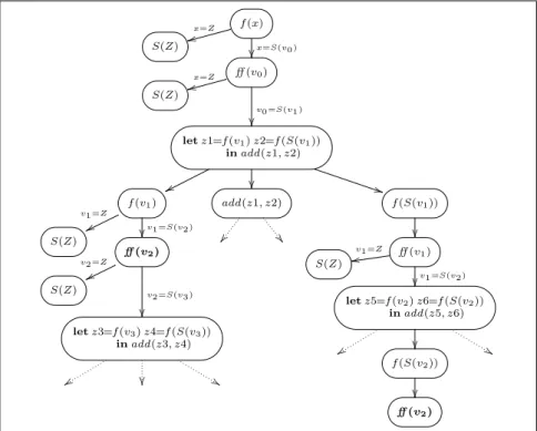
The actual program transformations in this paper were performed bySimple Su- percompiler(SPSC) [17]5, a clean implementation of a supercompiler with positive driving and generalization. The example programs are written in the object language of that system, a first-order functional language with normal-order reduction to weak head normal form [7]. All functions and constructors have a fixed arity. Pattern matching is only possible on the first argument of a function. For example, the function definition f(S(x), y) = f(x, y)is admissible, butf(x, S(y)) = f(x, y)andf(S(x), S(y)) = f(x, y)are not.
Example 1. Consider a functionf that returns its second argument unchanged if the first argument is the nullary constructorZand calls itself recursively if it has the unary constructorSas the outermost constructor. The function always returnsZas a result.
The computation of termf(x, x)in the start functionp(x)takes exponential timeO(2n) due to the nested double recursion in the definition off (here,n =|x|is the number
4Similar to partial evaluation, the result of a function call can be generalized by inserting let- expressions in the source program by hand (offline generalization) [2].
5SPSC home page http://spsc.appspot.com.
f(x, x)
x=Z
{{
x=S(v0)
((
Z f(f(v0, v0), f(v0, v0))
letv1=f(v0, v0)inf(v1, v1)
vv ))
f(v0, v0) f(v1, v1)
a) Driving with most-specific generalization: exponential speedup.
f(x, x)
x=Z
zz
x=S(v0)
**
Z f(f(v0, v0), f(v0, v0))
letv1=f(v0, v0)v2=f(v0, v0)inf(v1, v2)
tt **
f(v0, v0) f(v0, v0) f(v1, v2)
b) Driving without most-specific generalization: linear speedup.
Fig. 1.The partial process trees of a supercompiler with and without generalization.
ofS-constructors in the unary numberx). The residual programf1produced by SPSC takes timeO(n)on the same input, that is anexponential speedupis achieved.6
Source program Residual program
Startp(x) =f(x, x); Startp1(x) =f1(x);
f(Z, y) =y; f1(Z) =Z;
f(S(x), y) =f(f(x, x), f(x, x)); f1(S(x)) =f1(f1(x));
To understand what causes this optimization, compare the two process trees pro- duced by a supercompiler with and without generalization (Fig. 1a,b). In both cases, driving the initial terms=f(x, x)branches into two subtrees. One forx=Zand one forx=S(v0). Driving the left subtree terminates with termZ. In the right subtree each
6The speedup is independent of whether the programs are run in CBV, CBN or lazy semantics.