Windermere in relation to the estimate of the annual mean TP concentration (µg l) .66 Figure 6.9 Probability (PM) of misclassification of the ecological status of South Basin or.
Introduction
Project Objectives
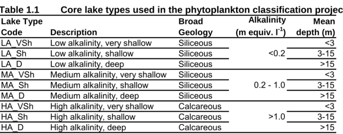
Lake types
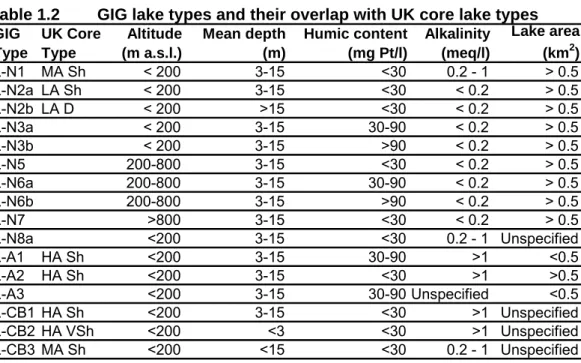
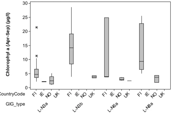
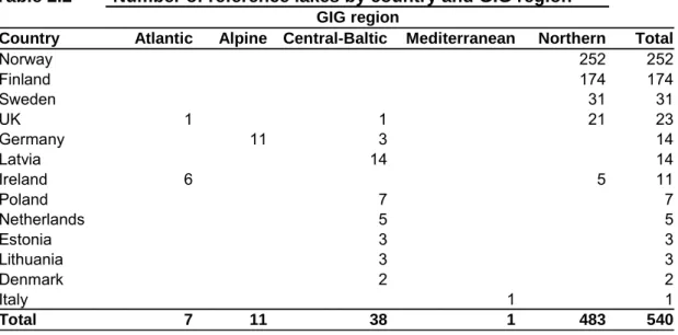
Some parts of the report mention the types of lakes used in the intercalibration process within these three GIGs. The overlap between these GIG types and the basic UK typology is detailed in Table 1.2. see Van de Bund et al., 2004 for a more detailed description of GIG lake types).
Chlorophyll reference conditions and the high/good boundary
Introduction
Historical data prior to watershed disturbance and paleolimology (transfer functions) are generally not available for determining reference chlorophyll concentrations, so the approach in this project is based on 1 and 2, both of which require a validated set of reference lakes. For this study, we collected data from UK reference lakes and also used data from >500 European reference lakes collected as part of Intercalibration and the EC Rebecca Project.
Methods
- Criteria for reference site selection
- UK data
- European data
- Descriptive statistics by lake type
- Correlation and regression models
Of the 61 reference lake catchments identified in Great Britain (GB), only 55 have chlorophyll data and many of these for only a single sampling occasion To minimize noise in the data set, lakes were only included in the analysis if they had three or more samples from different months between April and September. To minimize noise in the data set, lakes were included in the analysis only if they had three or more samples from different months between April–September (a 'growth period' in all lakes in the data set).
Results
- Descriptive statistics
- UK model
- European models
Correlation analysis indicated that colour, mean depth and alkalinity were likely to be the most important potential predictor variables, with height nearly significant (Table 2.10). This produced a model (r2adj = 0.27, r2pred = 0.26) with depth, alkalinity and elevation all identified as highly significant predictor variables (Table 2.11).
Discussion
- Descriptive Statistics
- UK chlorophyll model
- European chlorophyll models
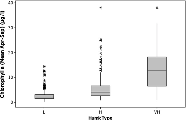
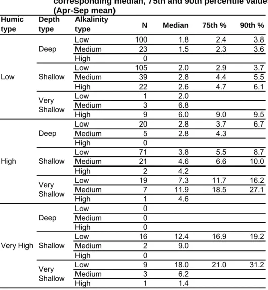
What the descriptive statistics do show is that chlorophyll reference conditions seem to increase with increasing humus content and, in particular, decreasing depth. Since chlorophyll concentrations in reference lakes appear to show gradients in response to the typological factors, a site-specific modeling approach may be more appropriate to establish reference conditions. For these reasons, it is highly recommended to use site-specific regression models to derive site-specific chlorophyll reference conditions.
The development of comparable regression models for setting reference conditions is well established for phosphorus, with the Morphodaphic Index model. Despite the relative success of the MEI model, no similar models have been published for setting chlorophyll reference conditions.
Summary and Recommendations
The significantly different relationship between chlorophyll-a and the predictor variables for low- and high-humic lakes highlighted the need to develop two separate models for these classes of lakes. Studies of boreal lakes have generally shown that phytoplankton biomass is lowest in clear water lakes (Arvola et al, 1999), but intuitively, chlorophyll concentrations would be expected to decrease with increasing color, due to reduced availability. of light for phytoplankton. In relation to the UK, regression models derived from UK reference lakes alone had significantly greater predictive power compared to the European models, and thus may be more appropriate in a UK context.
However, it should be noted that all the regression models should only be applied to lakes whose typology factors fall within the range covered by the model. Regression models derived solely from UK reference lakes had much greater predictive power compared to European models, and may therefore be more appropriate in a UK context, but they were based on a very limited data set and this should be noted that the models should only be applied to lakes whose typology factors fall within the range covered by the model.
Phosphorus reference conditions and the high/good boundary
- Introduction
- Methods
- UK data
- European data
- Descriptive statistics
- Correlation and regression models
- Results
- Descriptive statistics
- UK Model
- European models
- Discussion
- Recommendations
Data from 567 reference lakes met these conditions, with a large proportion of these sites coming from the Northern GIG region and having low alkalinity. TP data were pooled from a population of European reference lakes and the mean value within a lake type was adopted as the type-specific reference value, according to the REFCOND guidelines (Anonymous, 2003). Models were developed using independent predictors (Table 3.2) and using MEI and height as predictors (Table 3.3).
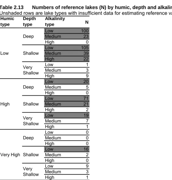
Regarding chlorophyll reference conditions, more efforts are needed to identify and sample a sufficient number of acceptable reference sites of these underrepresented lake types (Table 2.13) e.g. Further data collection should be carried out from UK reference lakes to better represent gradients of typology and improve the predictive power of the model.
Chlorophyll and light: defining the good/moderate boundary
Introduction
- Light attenuation
- The causes of attenuation
The attenuation of light through a uniform water column follows Beer's law (strictly this refers to a single wavelength): . ) ( 0exp K z. However, some areas will have much greater light attenuation for a given phytoplankton chlorophyll where suspended solids or dissolved organic carbon is high. For example, the phytoplankton of Esthwaite Water is the cause main light attenuation and there is a reasonable relationship between Secchi depth (very roughly, Kd = 1.44/Secchi depth) and phytoplankton chlorophyll a (Fig. 4.1a).
In contrast, Lake Bassenthwaite is a shallow lake where sediments are susceptible to wind disturbance, so total suspended solids can be high. As a result, Secchi depth can be very low even where phytoplankton chlorophyll is low (Figure 4.1b).
Methods
- Chlorophyll-specific attenuation
More recently, Krause-Jensen & Sand-Jensen (1998) reviewed data from 32 values in that literature and suggest an average of 0.015 m2 mg-1 vir phytoplankton chlorophyl a, and this is the value used here.
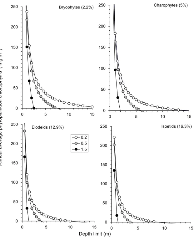
Results: phytoplankton chlorophyll concentration & macrophyte depth limit
Preliminary reference concentrations of phytoplankton chlorophyll a based on median values for reference lakes are shown in Table 4.2, as well as those at the good-moderate boundary which represent a doubling of the reference concentrations. In Table 4.3, the reference concentration of phytoplankton chlorophyll a is used to calculate reference depth limits for the different types of lake and macrophyte. Use the background attenuation coefficients in Table 4.1 and refer to phytoplankton chlorophyll a concentration in Table 4.2 and equation 4.
The only data in Table 3.5 not included in Figure 3.3 was the dataset from peat lakes (only shallow lakes available) because the method based on macrophyte colonization gave high estimates of chlorophyll concentration at the good-moderate boundary. Values based on reduction in macrophyte colonization depth (Table 3.5) and a doubling of reference chlorophyll concentration (Table 3.2).
Introduction
Methods
Thus, the analysis was based on seasonal averages derived from paired Chl TP and Chl TN for each lake. To determine relationships between Chlorphyll a and the supporting elements, TP and TN regression analysis was used (using SPSS). The significance of differences between type-specific conditions and the effects of other categorical variables, such as lake color, were tested using the general linear model routine.
Prior to analysis, data plots distributed by lake type were examined to determine apparent outliers that were removed from analysis. For the TN analysis all data from the UK were excluded as this determinant is not routinely used in the UK and the few data that were available were from new, invalid methods.
Results
- Descriptive statistics
- Regression relationships for core IC types
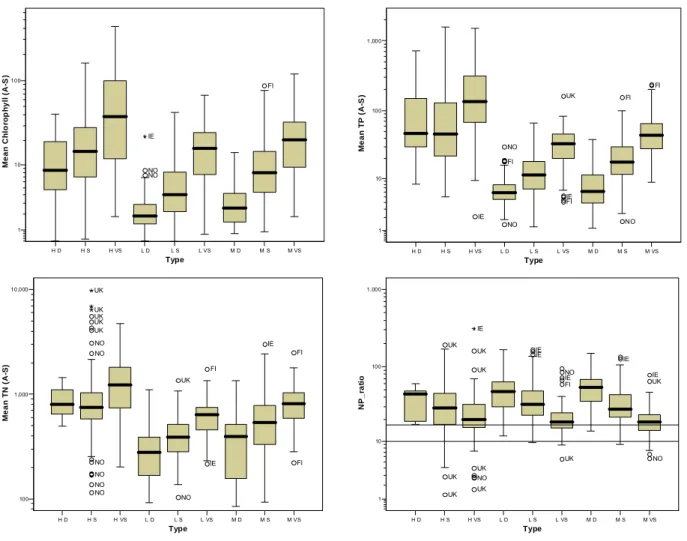
A scatterplot for total phosphorus and chlorophyll, showing the all-lake regression line and upper and lower bounds, is shown in Figure 5.5. Comparisons for lines that include 90% and 10% of data points for the chlorophyll total phosphorus relationship are also included. Regression relationships between total phosphorus and total nitrogen were determined for each of the core intercalibration types as shown in Table 5.2.
Regression equations for lake types that did not have significantly different regression equations for total phosphorus. However, ratios specific to the GIG type are also given for information. The range of chlorophyll, total phosphorus and total nitrogen is shown in Figures 5.9–5.11, and the regression equations for each type of GIG are shown in Table 5.4.
Discussion
Uncertainty in Chlorophyll-a and Total Phosphorus Classifications
- Introduction and approach
- Loch Leven
- South Basin of Windermere
- Implications for assignment of lakes to ecological status classes
- Use of STARBUGS
- Estimating uncertainty for other lakes
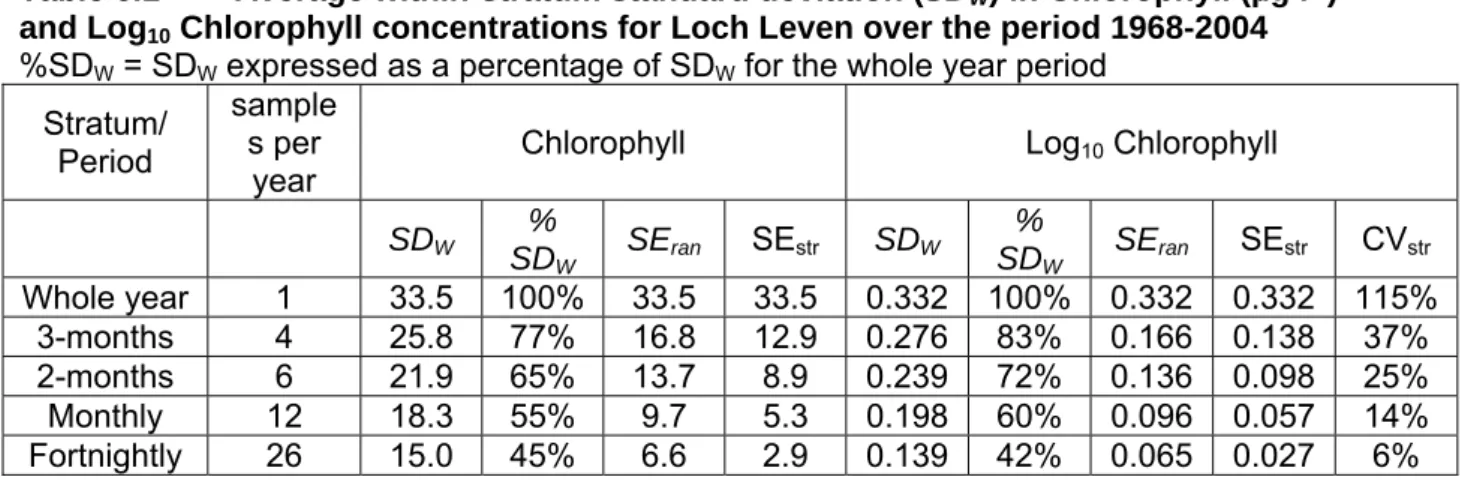
Each different sampling time would lead to (at least slightly) different estimates of the annual mean concentration. Variation within periods is now the only source of error in our estimates of the annual average. More specifically, for the current study of lakes, for any particular value of the estimate of the annual mean chlorophyll (or total phosphorus) concentration, the estimates of standard errors (SEstr in Tables 6.3-6.6) can be used to calculate the probability that the lake's true status class is different from its observed class based on estimate of annual mean.
This misclassification probability (PM) depends on the standard error (SEstr) of the estimate of annual mean, which depends on the sampling frequency over the year. These calculations are based on the assumption of a normal distribution for the sampling distribution of the estimator of the annual mean with a constant variance, regardless of the value of the estimate).
Summary and application of the classifications
- Reference Conditions
- High/Good Chlorophyll Boundary
- Good/Moderate Chlorophyll Boundary
- Total Phosphorus Boundaries
- Uncertainty and Data Issues
- Summary tables of reference conditions and boundary values
- Recommendations for further work
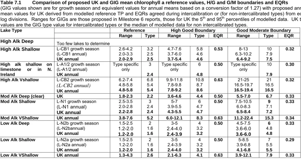
Originally, it was proposed that the H/G limit should be based on the 75th percentile of the modeled residuals of all UK lakes within each type. The EQR resulting from this limit is thus defined by intercalibration and will be used to establish the H/G limit for all UK sea types subject to intercalibration. For the non-intercalibrated lake types, EQR values were those derived from geometric divisions of the REBECCA data (Table 7.2).
It is proposed that the H/G cutoff for TP should be based on the 75th percentile of the residuals of the GB-calibrated MEI model. Different levels of precaution can be obtained by determining the TP value from the regression line or from lines based on different percentiles of the residuals of the regression.
The monitoring of ecological quality and the classification of standing water in temperate regions: A review and proposal based on an elaborated scheme for British waters. The loading concept as a basis for the control of eutrophication philosophy and preliminary results of the OECD program on eutrophication.
UK Reference lakes with sufficient chlorophyll data
Protocols for sample collection, storage and analysis