Synchronization: Stability and duration time

Synchronization: Stability and duration time

Laboratoire de Mecanique, Faculte´ des Sciences, Universite´ de Yaounde I, Boıˆte Postal 812, Yaounde, Cameroon 2_{Instituto de Fisica Teorica, Universidade Estadual Paulista, Rua Pamplona 145, 01405-900, Sa˜o Paulo, Brazil}

~Received 9 July 2001; published 5 March 2002!

We consider the problem of stability and duration of the synchronization process between self-excited oscillators, both in their regular and chaotic states. Making use of the properties of Hill equation describing the deviation between the slave and the master, we derive the stability conditions and expressions of the synchro-nization time. A fairly good agreement is obtained between the analytical and numerical results.

DOI: 10.1103/PhysRevE.65.036225 PACS number~s!: 05.45.Xt

I. INTRODUCTION

Synchronization of nonlinear oscillators both in their regular and chaotic states is presently one of the main re-search topics in the field of nonlinear science since the pio-neering work of Pecora and Carrol @1#. The great interest devoted to such a topic is not only due to the possibility of masking the information bearing signal by chaotic signals coming from electronic @1– 4#or optical @5– 8#sources, but also due to its applications in other fields, such as electrical and automation engineering, biology, and chemistry @9–12#. But despite the amount of theoretical and experimental results already obtained, a great deal of effort is still required to find optimal parameters to shorten the synchronization time, define the synchronization threshold parameters @13#, and to avoid loss of synchronization@14#and instability dur-ing the synchronization process. This problem is important in all the mentioned fields where synchronization finds or will find practical interest. For instance, as the communication is concerned, the range of time during which the chaotic oscil-lators are not synchronized corresponds to the range of time during which the encoded message can unfortunately not be recovered or sent. More than a grave and irreversible loss of information, this is a catastrophe in digital communications since the first bits of standardized bit strings always contain the signalization data or identity card of the message.

Here we aim to shed some light on this issue for oscilla-tors in their regular and chaotic states. The class of nonlinear oscillators, where the synchronization problem appears in the regular and chaotic states, is that of self-sustained oscillators. Recent studies on their synchronization process have been carried out and phenomena such as phase locking and cluster phase synchronization have been observed @15–17#. The classical van der Pol oscillator is a representative of self-sustained oscillators. It is described by the following equa-tion:

x¨₂d~12x2_!x˙

1x₅0, ~1!

where dots denote differentiation with respect to time. The quantity d is a positive parameter. This model is encountered in various fields: physics, electronics, and biology @18 –20#.

Its final state is a sinusoidal limit cycle for small d, develop-ing into relaxation oscillations when d becomes large. One particular characteristics of the van der Pol oscillator is that its phase depends on initial conditions, so that two identical van der Pol oscillators, set into motion with different initial conditions, will have the same amplitude and frequency, but have different phases.

In view of studying the phase locking or synchronization of two van der Pol oscillators, Leung considered recently various types of couplings including the continuous feedback difference coupling of Pyragas @21#. In particular, he ob-tained that synchronization is possible for some appropriate ranges of the coupling strength and that the synchronization time has a critical slowing down character near the bound-aries of the synchronization domain @22#. This study has been extended to generalized synchronization.

In this paper, we consider two points. We first show that the critical slowing down behavior of the synchronization time and the boundaries of the synchronization domain can be estimated, at least approximately by analytical consider-ations. The case of the relaxation oscillations is also carried out. For the second point, we extend the study to the syn-chronization process of two externally excited van der Pol oscillators in their chaotic state. This extension is important since recent studies showed that the critical and complex behavior of the synchronization time also appears for chaotic oscillators and the synchronization is more efficient only be-yond a critical value of the synchronization weight @9,25#. One would like to know if some aspects of this complex behavior can be explained analytically.

The organization of the paper is as follows. In the follow-ing section, we study analytically the stability of the syn-chronization process and derive expressions of the synchro-nization time. The analytical results are then compared to the numerical ones. In Sec. III, we extend the investigation to the synchronization of two forced van der Pol oscillators in a chaotic state. Section IV is devoted to the conclusion.

II. STABILITY AND SYNCHRONIZATION TIME

A. Stability of the synchronization process

with different phasesf1 andf2. To phase lock so thatf1

2f250, the good strategy is to use the conventional feed-back scheme in the following manner:

x¨₂d~1₂x2_!x˙

1x₅0, ~2a!

u¨₂d~12u2_!u˙

1u₅K~u₂x!H~t₂T₀!, ~2b!

where K is the feedback coupling coefficient or strength and H the Heaviside function defined as

H~x!50 for x_,0 and H~x!51 for x>0.

t is the time and To is the onset time of the synchronization process. Here x is called the master and u the slave. The role of the feedback is thus to force the convergence of the slave towards the master orbit.

When the synchronization process is launched, the slave configuration changes and one would like to determine the range of K for the synchronization process to be achieved, and for the dynamics of the slave to remain stable. To carry out such an investigation, let us introduce the variable

z₅u₂x, ~3!

which is the measure of the nearness of the slave to the master. Introducing z in Eq.~2b!and considering only linear terms, we obtain the following equation:

z¨₂d~12x2!z˙₁~2dxx˙₁1₂K!z₅0. ~4!

The synchronization is achieved when z goes to zero as t increases or, practically, is less than a given precision. The behavior of z depends on K and on the form of the slave x. Assuming small d, the master dynamics can be described by

x₅A cos~vt₂f1!, ~5!

where the amplitude A and the frequencyvdepend on d. If we let t5vt₂f1, the variational equation ~4! takes the form

z¨₁@2l₁F1~t!#z˙₁G~t!z₅0, ~6!

where

F1~t!5 A2 2vcos 2t,

G~t!512K2dA

2_{cos 2t}

v2 ,

and

l₅ 1

2v

S

A2 221

D

From the expression of G(t), we find that if K_.1, z will grow indefinitely leading the slave to continuously drift away from its original limit cycle. In this case, the feedback coupling is dangerous since it continuously adds energy to the slave system. This boundary, obtained here from the

simple analytical consideration, has been observed by Leung @22,23#, in its numerical simulation of Eq.~2!. We note that this critical value of K also works in the case of relaxation and chaotic oscillations.

To discuss further the stability process, let us rewrite Eq. ~6!in a standard form. For this purpose, we use the transfor-mation

z₅W exp~2lt!exp

S

2

E

D

W¨1~a012a1ssin 2t12a1ccos 2t12a2ccos 4t!W50 ~8!

with

a05 1

vz

F

4

S

2 21

D

2d

2_A4

32

G

2dA2 dv ,

a1c5

2d2

16v2~~A222!A2!, a2c5

2d2A4 64v2 .

Equation ~8!presents two main parametric resonances at a0

5n2~with n₅1, 2!. The stability boundaries of the synchro-nization process are to be found around these two reso-nances. For this purpose, we use the Whittaker method@18#. We assume that at the nth unstable region, the solution of Eq. ~8!has the following form:

W₅emrsin~nt2s!, ~9!

where m is the characteristic exponent and s a parameter. Substituting Eq. ~9!into Eq.~8!and equation coefficients of sin(nt) and cos(nt), we find that the expression of the char-acteristic exponent is

m2

52~a₀₁n2_!

1

A

2

with

a_n2₅a_ns2 ₁a_nc2 .

From the transformation~7!, it comes that for z to tend to zero with increasing time, the real parts of2l₆mshould be negative. Consequently, the synchronization process is stable under the condition~assuming thatmis real!

~a02n2!212~a01n2!l21l4.an 2

with n51,2. ~10!

We have checked for the validity of these criteria by solving numerically Eq. ~2! for d₅0.3 and d₅1. The values of A andvare resorted from the numerical simulation. In the case d50.3, we obtain from Eq. ~10! that the synchronization process is unstable for K_P@20.09,0# ~and obviously for K

.1!. We note here that the synchronization process is

d51 ~the parameter used in Ref.@22#!, it is found from our analytical consideration that the synchronization process is unstable for K_P@21.03,0# while the numerical simulation gives K_P@20.39,0#. Here we find a deviation between the analytical and numerical results. This deviation is under-standable since the analytical investigation assumes small d and a pure sinusoidal form for the master x. This is not exactly the case for d51. One could expect that the agree-ment between the analytical and numerical results can be improved if instead of using only one harmonics, one con-siders more so that the analytical form of x is closer to the exact profile of x. However, despite the deviation, the pure sinusoidal approximation still presents other stability bound-aries and the range where the synchronization could be at-tained more quickly.

B. The synchronization time

For practical purpose, having an analytical expression re-lating the synchronization time to the synchronization strength and other parameters of the physical system is inter-esting, since it gives not only an estimate of the synchroni-zation time for a given set of parameters, but also a way to monitor the synchronization by adjusting the coupling strength. In this section, we derive expressions for the syn-chronization time from the variational Eqs.~6!and~8!.

There are two ways to compute the synchronization time. The first way is to follow the time trajectory of the slave system relative to that of the master. In this case, synchroni-zation is achieved when the deviation z obeys the following condition:

uz~t!u,h ; t.ts, ~11a!

where h is the synchronization precision or tolerance. The second way is to follow the orbit of the slave in the phase space. Here the synchronization criterion is

A

1~n2y!2

,h ; .ts, ~11b!

where y and v are the velocities of the master and slave,

respectively. Our analytical calculation leads to the same ex-pression for the synchronization time for both equations. In both cases, the synchronization time is defined as

T_s5t_s2T₀. ~11c!

Returning now to the variational equation~8!, near the reso-nant state, z takes the form

z~t!5$c1exp@2~ l2m!t#sin~nt2s1!

1c2exp@2~ l1m!t#sin~nt2s2!%

3exp

F

2

E

G

where c₁ and c₂ are two constants depending on initial con-ditions for z. Since the term proportional to c2 decreases more quickly, we only consider the first term and obtain that

c₁2₅z₀2₁

S

D

2 ,

where z0 and z˙0 are the values of the deviation and its ve-locity at the time T0 when the synchronization process is launched. Consequently, following Eq. ~11a! or ~11b!, it comes that near the resonances, the expression of the syn-chronization time is defined by

T05 1 l₂mln

c1

h . ~12!

Far from the resonant states, the variational equation reduces to

z¨₁2lz˙₁V₀2_z

50, ~13!

where V₀2₅(1₂K)/v2_{. This is simply the equation of a} damped harmonic oscillator whose solution depends on the sign of D₅V₀2₂l2_{. Following the procedure used above,} we find that the synchronization time has the following ex-pressions. For D_.0, we have

T₀₅1 lln

b0

h, ~14a!

with b₀2₅z₀2₁z˙0 2

D,

and forD_,0, we have

T05 1

A

h, ~14b!

with c05

A

2

A

We have checked for the validity of these analytical results by comparing the values given by Eqs.~12!and~14!to those obtained from the numerical simulation. The numerical simulation uses the fourth-order Runge-Kutta algorithm with a time stepDt50.01. We use Eq.~11b!to compute the syn-chronization time with the precision h₅1025.

of Tsin the case of relaxation oscillations (d55). It is found that the variation of K in the range@21.70, 1#has a complex hatched structure with various domains of no synchroniza-tion ~Fig. 3!. But even here, when K is large, the analytical formula for Ts @Eq.~14a!#gives results comparable to that of the numerical simulation ~Fig. 4!.

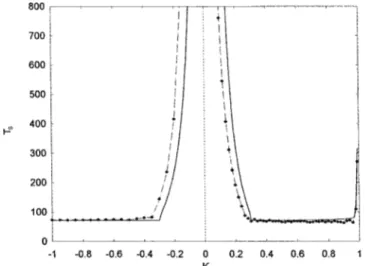
From the analytical expressions of T_s, we can resort the following comments. First, the agreement between the ana-lytical and numerical results clearly indicates that, at least for small d, the slowing down behavior of Tsas K varies is well described by the analytical expressions ~12! and~14!. Sec-ond, our expressions indicate how the synchronization time is related to the synchronization onset time and on the toler-ance h. Third, from Eq.~14a!, we see that asuKuincreases, T_s decreases towards a minimal limiting value

Ts5 1 lln

uz0u

h , ~15!

which is independent of the synchronization coupling strength K, but depends on the tolerance h. Hence Eq. ~15!

gives an incompressible asymptotic duration below which no synchronization can be obtained however much we increase the value of K.

III. SYNCHRONIZATION OF TWO FORCED CHAOTIC OSCILLATORS

We have extended the analysis of the synchronization to two nonautonomous van der Pol oscillators described by conventional feedback scheme in the following manner:

x¨2d~12x2!x˙1x5E cosVt, ~16a!

u¨₂d~1₂u2!u˙₁u₅E cosVt₁K~u₂x!H~t₂T0!, ~16b!

where E and V are, respectively, the amplitude and fre-quency of the external excitation. A similar study had already been carried out for Duffing oscillators @24,25#. The objec-tive of this extension is to see how the synchronization time evolves for chaotic van der Pol oscillators and to what extent the analytical investigation of Sec. II could be of any help for the synchronization of chaotic process in general.

FIG. 1. Synchronization time versus K for d50.3: numerical results~lines with dots!and analytical results~lines!.

FIG. 2. Same as Fig. 1 for d51.

FIG. 3. Numerical values of the synchronization time versus K for d55.

As it is known, chaos is not very abundant in Eq.~16a!. In Ref.@26#, it had been shown that chaos appears only for high values of d and E, and in a limited range of the frequencyV. Typically, with d₅E₅5, chaos is found in the range V

P@2.463,2.466#. Here we use V52.465. The

synchroniza-tion time vs K is reported in Fig. 5 for K,23.4~the range where the synchronization is more efficient!. In the domain KP@23.4,1#, various intervals ~sometimes reduced to a single value of K with a stepDK₅0.01!of synchronization alternate with that of no synchronization. This is a domain to avoid. This qualitative behavior resembles the one obtained in Ref.@25#for the synchronization of chaotic Duffing oscil-lators.

As concerns the analytical investigation, we are obviously limited by the fact that a chaotic orbit is aperiodic and is composed of an infinite number of orbits. However, to evalu-atelin Eq.~6!for the calculation of Ts given by Eq.~14a!, we have used the value A₅1.757. This amplitude can be obtained by finding a solution defined by Eq. ~5! with an analytical approximate method ~e.g., the harmonic balance method!for nonlinear oscillators applied to Eq.~16a!. Using this value and the frequencyV₅2.465~in place ofv!in the formula ~14a!, we obtain the results reported in Fig. 5 ~dashed line!. This shows that even for the synchronization of chaotic oscillators, we can predict the K dependence of the synchronization time when K is large by using Eq. ~14a!.

Moreover, the analytically predicted critical value K51, is also valid here so that launching the synchronization of two chaotic van der Pol oscillators with K_.1 will drive continu-ously the slave from the master ~and practically leads to harmful consequences since the slave amplitude grows in-definitely!.

IV. CONCLUSION

This paper has considered the question of an analytical determination of the stability boundaries and duration time for the synchronization of two nonlinear oscillators in the regular and chaotic states. The model used is the classical van der Pol oscillator, which shows dependence on initial conditions in its regular and chaotic states. The analytical investigation is based on the properties of the Hill equation, which described the deviation between the slave and the master oscillators. We have found the synchronization boundaries and derive the expressions for the synchroniza-tion time. We have found good agreement between the ana-lytical and numerical results, in particular, in cases of a small nonlinear coefficient where the state of the master can be described by a sinusoidal wave form. The extension to syn-chronization of chaotic oscillators gives a hint for the deter-mination of necessary and sufficient conditions for high-quality synchronization of chaotic systems. Indeed, our recent analytical investigation of the same question in the case of synchronization of chaotic single-well Duffing oscil-lators shows that when the chaotic attractor possesses a single strong spectral component, the analytical procedure based on the variational equation gives good results for the boundaries and duration of the synchronization process. We expect that this analytical procedure could give an alternative way, besides the numerical calculation of the Lyapunov spec-trum of the slave system@1#, to optimize the synchronization process even in the model described by first-order differen-tial equations, such as Rossler and Lorenz oscillators.

ACKNOWLEDGMENTS

P.W. is grateful to FAPESP ~BRASIL! for financial sup-port and to Instituto de Fisica Teorica-Unsep, Sa˜o Paulo, Brazil for hospitality. The authors are grateful to A. Kam-chatnov and B. A. Umarov for helpful and stimulating dis-cussions.

@1#L. M. Pecora and T. L. Carroll, Phys. Rev. Lett. 64, 821 ~1990!; Phys. Rev. A 44, 2374~1991!; Int. J. Bifurcation Chaos Appl. Sci. Eng. 2, 659~1992!.

@2#A. V. Oppenheim, G. W. Wornell, S. H. Isabelle, K. Cuomo, in Proceedings of the International Conference on Acoustic, Speech and Signal Processing~IEEE, New York, 1992!, Vol. 4, p. 117.

@3#L. J. Kocarev, K. S. Halle, K. Eckert, U. Parlitz, and L. O. Chua, Int. J. Bifurcation Chaos Appl. Sci. Eng. 2, 702~1992!. @4#K. M. Cuomo and A. V. Oppenheim, Phys. Rev. Lett. 71, 65

~1993!.

@5#H. G. Winful and L. Rahman, Phys. Rev. Lett. 65, 1575 ~1990!.

@6#R. Roy and K. S. Thornburg, Jr., Phys. Rev. Lett. 72, 2009 ~1994!.

@7#S. Sivaprakasam and K. A. Shore, Phys. Rev. E 61, 5997 ~2000!.

@8#A. Murakami and J. Ohtsubo, Phys. Rev. E 63, 066203~2001!, and references therein.

@9#P. Woafo, Phys. Lett. A 267, 31~2000!.

@10#A. T. Winfree, The Geometry of Biological Time ~ Springer-Verlag, New York, 1980!.

@11#Y. Kuramoto, Chemical Oscillations, Waves and Turbulence ~Springer-Verlag, Berlin, 1984!.

@12#M. Bazhenov, R. Huerta, M. Rabinovitch, and T. Sejnowski, Physica D 116, 392~1998!.

@13#K. Pyragas, Phys. Rev. E 58, 3067~1998!. @14#N. J. Corron, Phys. Rev. E 63, 055203~2001!.

@15#G. V. Osipov, A. S. Pikovsky, M. G. Rosenblum, and J. Kurths, Phys. Rev. E 55, 2353~1997!.

@16#Z. Zheng, B. Hu, and G. Hu, Phys. Rev. E 62, 402~2000!. @17#T. E. Vadivasova, G. I. Strelkova, and V. S. Anishchenko,

Phys. Rev. E 63, 036225~2001!.

@18#C. Hayashi, Nonlinear Oscillations in Physical Systems

~McGraw-Hill, New York, 1964!.

@19#J. M. T. Thompson and H. B. Stewart, Nonlinear Dynamics and Chaos~Wiley, New York, 1986!.

@20#O. Kongas, R. V. Hertzen, and J. Engelbrecht, Chaos, Solitons Fractals 10, 119~1999!.

@21#K. Pyragas, Phys. Lett. A 170, 241~1992!. @22#H. K. Leung, Phys. Rev. E 58, 5704~1998!. @23#H. K. Leung, Physica A 281, 311~2000!. @24#T. Kapitaniak, Phys. Rev. E 50, 1642~1994!. @25#G. Malescio, Phys. Rev. E 53, 2949~1996!.