Features of annual and semiannual variations derived from the global ionospheric maps of total electron content

www.ann-geophys.net/25/2513/2007/ © European Geosciences Union 2007

Annales

Geophysicae

Features of annual and semiannual variations derived from the

global ionospheric maps of total electron content

B. Zhao1, W. Wan1, L. Liu1, T. Mao1,2,3, Z. Ren1,2,3, M. Wang1,2.3, and A. B. Christensen4

1_{Institute of Geology and Geophysics, Chinese Academy of Sciences, Beijing 100029, China} 2_{Wuhan Institute of Physics and Mathematics, CAS, Wuhan 430071, China}

3_{Graduate School of Chinese Academy of Sciences, Beijing, China}

4_{Space Science Applications Laboratory, Aerospace Corporation, El Segundo, California, USA}

Received: 26 January 2007 – Revised: 23 July 2007 – Accepted: 25 October 2007 – Published: 2 January 2008

Abstract.In the present work we use the NASA-JPL global ionospheric maps of total electron content (TEC), firstly to construct TEC maps (TEC vs. magnetic local time MLT, and magnetic latitude MLAT) in the interval from 1999 to 2005. These TEC maps were, in turn, used to estimate the annual-to-mean amplitude ratio, A1, and the semiannual-annual-to-mean amplitude ratio,A2, as well as the latitudinal symmetrical and asymmetrical parts,A′andA′′ofA1. Thus, we investi-gated in detail the TEC climatology from maps of these in-dices, with an emphasis on the quantitative presentation for local time and latitudinal changes in the seasonal, annual and semiannual anomalies of the ionospheric TEC. Then we took the TEC value at 14:00 LT to examine various anomalies at a global scale following the same procedure. Results reveal similar features appearing in NmF2, such as that the seasonal anomaly is more significant in the near-pole regions than in the far-pole regions and the reverse is true for the semian-nual anomaly; the winter anomaly has least a chance to be observed at the South America and South Pacific areas. The most impressive feature is that the equinoctial asymmetry is most prominent at the East Asian and South Australian areas. Through the analysis of the TIMED GUVI columnar [O/N2] data, we have investigated to what extent the seasonal, annual and semiannual variations can be explained by their counter-parts in [O/N2]. Results revealed that the [O/N2] variation is a major contributor to the daytime winter anomaly of TEC, and it also contributes to some of the semiannual and annual anomalies. The contribution to the anomalies unexplained by the [O/N2] data could possibly be due to the dynamics associated with thermospheric winds and electric fields.

Keywords. Atmospheric composition and structure (Thermosphere-composition and chemistry) – Ionosphere (Mid-latitude ionosphere, Equatorial ionosphere)

Correspondence to:B. Zhao ([email protected])

1 Introduction

equinoctial asymmetries (the electron density in one equinox being larger than that in the other equinox) in the ionosphere and thermosphere during solar maximum period by using the Japanese MU radar data. Ma et al. (2003) derived features of the semiannual anomaly at different latitudes and longitudes using worldwide ionosonde data from 1974–1986.

Many theories have been proposed to explain the varia-tions of the F2-layer anomalies, as reviewed by Rishbeth (1998). Among these various theories, the “chemical expla-nations” proved to be rather reasonable and have been ac-cepted to some extent. Rishbeth and Setty (1961) and Wright (1963) recognized that the change in the chemical composi-tions in the upper atmosphere, such as the atomic–molecular ratio [O/N2], could mainly account for the variation of NmF2 during the daytime. Subsequently, Johnson (1964) and King (1964) suggested that the thermospheric circulation from the summer hemisphere to the winter one could affect the [O/N2] ratio and finally change NmF2. Since the 1980s, numerical methods have been applied to investigate the electron den-sity variations in the ionosphere. Based on the global ther-mospheric circulation theory, Fuller-Rowell and Rees (1983) reproduced the seasonal variation of NmF2. After consider-ing the offset of the geographic and geomagnetic poles, Mill-ward et al. (1996) tried to explain the longitude differences in seasonal and semiannual characteristics at mid-latitudes. Fuller-Rowell (1998) proposed a mechanism named “ther-mospheric spoon” to interpret the semiannual variation in the ionosphere. He suggests that the global-scale, interhemi-spheric circulation at solstices acts like a huge turbulent eddy in mixing the major species. The effect causes less diffusive separation of the species at solstices, which tends to a rise in the molecular nitrogen and oxygen densities and a reduction in the atomic oxygen density. With a coupled thermosphere-ionosphere-plasmasphere model (CTIP), Zou et al. (2000) re-examined the global thermospheric circulation theory and how far the semiannual anomaly could be explained by this theory without invoking other causes. Thereafter, Rishbeth et al. (2000) gave a detailed physical discussion.

Hitherto, most studies of the F-layer anomaly have used data on NmF2 from ionosonde stations (e.g. Yonezawa, 1971; Torr and Torr, 1973; Yu et al., 2004). However, some measurements have shown that these anomalies vary at dif-ferent altitude regimes. Observational evidence indicates that there is no winter anomaly in the topside ionosphere, whereas it is significant in the F-region (e.g. Balan et al., 1998; Torr and Torr, 1973; Su et al., 1998; Zhao et al., 2005; Liu et al., 2007). Moreover, observational evidence also shows that the annual anomaly is very strong in the topside ionosphere, as compared with the bottomside ionosphere (Su et al., 1998). It is reasonable to imagine that the total elec-tron content (TEC) and the integral of elecelec-tron density height profile N(h) might have different characteristics as compared with those derived from the NmF2. Further support is pro-vided by the fact that the annual anomaly predominates over the seasonal variations for TEC (Titheridge and Buonsanto,

1983) compared to the small annual component for NmF2. In recent years, a database of TEC in the ionosphere and plasmasphere, derived from a worldwide network of global positioning system (GPS) observations, has been used to investigate the local and regional characteristics of various anomalies (Huang and Cheng et al., 1996; Unnikrishnan et al., 2002; Wu et al., 2004). Since the early 1990s, a worldwide network of permanent GPS tracking stations has rapidly grown under the management of the International GNSS (Global Navigation Satellite Systems) Service, known as IGS. In May 1998, IGS created the Ionosphere Working Group (Feltens and Schaer, 1998), and soon after five differ-ent cdiffer-enters started computing and making available several GPS-derived ionospheric products, mainly two-dimensional world-wide grids of vertical total electron content (VTEC) and differential code biases (DCBs) for every satellite and many receivers in the network. To make feasible inter-changes and comparisons, the so-called IONEX (Ionosphere Map Exchange) standard format was established (Schaer et al., 1998). In this study, we use the global ionospheric maps (GIMs) developed by the JPL because of its relatively high reliability and accuracy. There is a rich literature describing the development of JPL GIM (e.g. Mannucci et al., 1998), as well as their use in studies of ionospheric behavior, partic-ularly under disturbed conditions (Ho et al., 1996; Pi et al., 1997). The GPS system and the JPL GIMs derived from its data have become a standard ionospheric diagnostic tool, and are particularly useful for our study.

Mendillo et al. (2005) have found the annual anomaly in TEC to be a global characteristic by using GIMs data of the year 2002. Here, to some extent, we are about to expand their work and explore the global feature of the principle F2-layer anomalies, including the winter anomaly, the semian-nual anomaly and the ansemian-nual anomaly. First, we have at-tempted to find out how these anomalies varied under differ-ent magnetic local time (MLT) and differdiffer-ent solar activity, in which we compare them with the magnitudes of the annual and semiannual anomaly by using data from the GUVI ex-periment aboard the TIMED satellite. Then we studied the global distribution of the amplitudes of various anomalies during the daytime under different solar activity. In the Dis-cussion section, current theories and mechanisms were used to give possible explanations of various anomalies. We hope the work could help us in achieving comprehensive insight into the complexities of F2-layer behavior.

2 Magnetic local time variation of the anomalies

2.1 Data resources and analysis method

A

Fig. 1.An example of GIM being transformed from an Earth-fixed geographic frame into a MLAT-MLT frame at 01:00 UT on 1 Jan-uary 2000.

the fact that each new daily file contains ionospheric infor-mation covering not only 22 but 24 h. The new daily file in-cludes 13 VTEC maps, starting from 00:00 UT to 24:00 UT, in order to facilitate the data interpolation. Each map is cre-ated in an Earth-fixed reference frame with geographic longi-tude ranging from−180◦to 180◦(5◦resolution) and latitude from−87.5◦ to 87.5◦(2.5◦resolution). For our purpose in constructing TEC maps, we follow the works of Codrescu et al. (2001) and Jee et al. (2004) to estimate the TEC maps in the plane of magnetic local time (MLT) vs. magnetic lat-itudes (MLAT) using quasi-dipole coordinates (Richmond, 1995). Thus, we first transform the geographic longitude and latitude into MLT (00:00∼24:00) and MLAT (−70◦∼70◦), and then divide the MLT vs. MLAT plan into mesh grids with grid length dMLT=0.5 hour and dMLAT=2.5◦. We calculate the average TEC in each bin as the grid TEC values. We estimate the TEC maps in the plane of magnetic local time (MLT) vs. magnetic latitudes (MLAT) by virtue of the tilted dipole field. Figure 1 gives an example of GIM being trans-formed from an Earth-fixed into a MLAT-MLT frame. The most prominent feature of the TEC maps is the well-known double crest structure of the ionospheric equatorial anomaly. The equatorial anomaly crests usually appear in the magnetic latitude about±10◦∼15◦ during almost the entire daytime, with a maximum value at post noon. For each day there are 12 or 13 maps and we make an average to give one map a day which is enough for the investigation of the ionospheric cli-matology. To extract the amplitudes of the annual and semi-annual variations, a yearly TEC variation is represented by the sum of the yearly average TEC0, annual TEC1 and semi-annual TEC2 components:

TEC(mlat, d)=TEC0+TEC1+TEC2

=TEC0{1+A1×cos[2π(d−d1)/T]

+A2×cos[4π(d−d2)/T]}

(1)

A1=TEC1/TEC0;A2=TEC2/TEC0;

wheredis the day number andT (T=365, and 366 for leap year) is the total days of a year. TEC0 is the yearly average

A

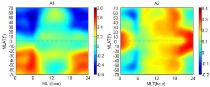
Fig. 2.Annual and semiannual indicesA1andA2for the year 2000

have been estimated as functions of MLT and MLAT, according to the Eq. (1). In the left panel of Fig. 2, positive values indicate that the maximum value of the yearly TEC appears at the December solstice and negative denotes the June solstice.

value of TEC.A1andA2are, respectively, the relative am-plitudes of the TEC annual and semiannual components;d1 andd2are the corresponding phases, respectively, denoting the winter solstice and vernal equinox and vary slightly from year by year. For the year 1999, 2002 and 2003, d1 is 22 December and for the remaining year 21 December. For the year 1999 and 2003,d2is 21 March while for the remaining year 22 March.

2.2 Results of the GIM

Displayed in Fig. 2 are the annual and semiannual indices,

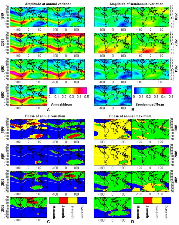
Fig. 3a. Distribution of (a) symmetrical index A′, defined as

(A1(MLAT)−A1(−MLAT))/2(b)asymmetrical indexA′′, defined

as (A1(MLAT)+A1(−MLAT))/2 and(c)semiannual componentA2

for the year 1999–2005.

latitude, meeting the subsidiary circulation that originated from the winter auroral oval. The downwelling air will in-crease the [O/N2] and dein-crease the mean molar mass,thus increasing the electron content (Rishbeth, 1998). The right panel of Fig. 2 depicts the variation of the semiannual index

A2, which has a clear latitudinal and local time dependence. Generally, there is a small, semiannual background compo-nent distributed from equatorial region to the high latitudes. However, a significantA2occurs after 12:00 MLT, where the maximum value appears at sub-equatorial regions during the period 20:00–24:00 MLT. To further explore the characteris-tics of the various anomalies, we define the symmetrical and asymmetrical indices as A′=(A1(MLAT)−A1(−MLAT))/2 andA′′=(A1(MLAT)+A1(−MLAT))/2, in which the former denotes the amplitude of the seasonal variation and the latter represents the annual anomaly. Thus, plentiful properties of the ionospheric TEC climatology were found in these index maps from the year 1999 to 2005, as shown in Fig. 3.

The distribution ofA′, shown in Fig. 3a, manifests that the noon winter anomaly has a clear solar activity dependence. During the low solar activity year, the noon anomaly at mid-latitudes is absent, withA′′being negative. At moderate so-lar activity, for example 1999 and 2003,A′′is no more than 5% (5% means 0.05 and the same for the following value)

Fig. 3b.Continued.

2.3 Results in neutral O/N2 from GUVI observations We take as a first approximation that photochemical equilib-rium conditions prevail up to the F-region peak. In this case the maximum ionization is given by Nmax∼q/β∼[O/N2] (Rishbeth, 1998). In this study, we want to find out whether the neutral gas composition at F-layer heights has the sea-sonal, semiannual and annual anomalies of the comparable magnitude, as that which appears in the TEC, without con-sidering the effects of the transport processes. We use the [O/N2] data measured from the global ultraviolet imager on the TIMED satellite (Christensen et al., 2003). The values of [O/N2] refer to column density ratios above levels of the fixed N2 column content (1021m−2 or 1017m−2), derived from airglow observations in the 140–250 km height range; see Christensen et al. (2003) and Strickland et al. (2004) for details of the experiment and analysis techniques. Strickland et al. (2001) showed that the electron concentration varies with this column density ratio. These are shown as global maps in Strickland et al. (2004), depicting the global distri-bution of columnar [O/N2] at local noon on four particular days in 2002–2003, which were geomagnetically quiet, and have similar levels of solar flux index F107.

The TIMED satellite was launched on 7 December 2001 into a 630 km, 74.1◦inclination circular orbit with a 97.8 min period. The orbital precession rate is such that the beta an-gle (the anan-gle between the Earth-Sun vector and the orbital plane) passes through zero every 120 days, so the local time of the orbit varies with this periodicity. As a consequence, GUVI samples all local solar times every 60 days, counting ascending and descending node orbits. The data have been transformed into the MLAT vs. MLT frame and a 60-day moving average has been employed to preserve the spatial and temporal information. Four years of data during 2002– 2005 have been utilized to extract the seasonal, semiannual and annual amplitudes with Eq. (1). Figure 4 gives the dis-tribution of the columnar [O/N2] centered at equinox and solstice during the year 2003. The distribution presents a clear seasonal variation which shows that [O/N2] is low in the summer hemisphere and high in the winter hemisphere at middle-high latitudes. Data during the 08:00–16:00 MLT interval is shown with full resolution, to facilitate the study of various anomaly changes.

Figure 5 displays the magnitudes of the symmetrical index

A′, the asymmetric index A′′ and the semiannual variation

A2for [O/N2] from 2002 to 2005, respectively. The mag-nitude of A′ has a clear solar dependence that varies from 0.3–0.45 with increased solar activity, and is much larger than that for the winter anomaly in TEC. This is probably because the daytime summer-to-winter wind will reduce the winter anomaly effect by uplifting and depressing the F-layer peak. The difference may also partly result from the differ-ent height range measured for these two parameters. The overall value of the distribution ofA′′is∼0.1, less than that of TEC at ∼0.15, which partly can be used to explain the

Fig. 3c.Continued

Fig. 4.Distribution of the columnar [O/N2] centered at equinox and solstice during the year 2003.

′ ′′

A′

A′′

A₂

Fig. 5.From the top to bottom panel are the magnitudes ofA’,A′′andA2for GUVI [O/N2] during 08:00–16:00 MLT from 2002 to 2005,

respectively, corresponding to Fig. 3a, b and c.

northern mid-high latitudes is weaker than that in the South-ern Hemisphere. This feature can be also identified in the distribution ofA2in TEC, as shown in Fig. 3c at around the MLT=12:00 sector in the mid-high latitude. It is understood that the results of the TEC and [O/N2] are sometime uncorre-lated because we do not consider the transport process. The ionosphere is not only controlled by the solar zenith angle but also constrained by the magnetic field. For example, a strong semiannual variation at the double crest region after

sunset may be associated with the semiannual variation of the equatorialE×B drift. Detailed discussion is given in the Discussion section.

3 Longitude variation of the annual and semiannual variation at 14:00 LT

anomalies. As is shown in the above section, the winter anomaly is most pronounced during 14:00 LT, so we take the TEC value at 14:00 LT to examine various anomalies at a global scale. The analysis of the data is the same as the previous local time variation by applying Eq. (1) but without limiting the phasesd1andd2. Equation (1) can be expanded by the following form:

TEC(mlat, d)=TEC0{1+A1×cos[2π(d−d1)/T]

+A2×cos[4π(d−d2)/T]

=TEC0{1+C1×cos[2π d/T] +C2×cos[4π d/T] +S1×sin[2π d/T] +S2×sin[4π d/T]}.

(2)

A1= q

C₁2+S₁2andd1=tan−1(S1/C1)are the amplitude and phase of annual variation, respectively, and A2=

q C₂2+S₂2

andd2=tan−1(S2/C2)are the amplitude and phase of the semiannual variation, respectively. We use the method of regression analysis to calculate the amplitudes and phases of the semiannual variation.

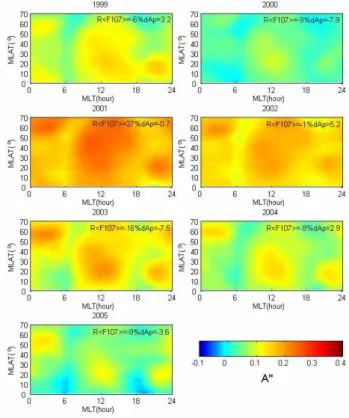
Panels (A) and (B) of Fig. 6 illustrate the relative ampli-tudes of the annual and semiannual variations. Panel (C) shows the phase of the annual variation (C) and panel (D) gives the phase of maximum value of TEC. Here we did not display the phase of the semiannual variation becaused2is during either a vernal month or an autumnal month, which provides no valuable information. In order to facilitate our description, we define March, April and the first half part of May asM-month. June, July, August and the last half part of May are denoted asJ-month, and September, Octo-ber and the first half part of NovemOcto-ber asS-month, and De-cember, January, February and the last half part of Novem-ber asD-month. In panels (C) and (D), different areas are filled with different colors according to their phase distribu-tion. Combining (A)–(C), we note the following features: (1) the amplitude of the winter anomaly is prominent at middle and mid-high latitudes in the Northern Hemisphere, which is clearly modulated by the solar activity. More area is cov-ered with the winter anomaly at Northern Hemisphere during higher solar activity year. The most striking area of winter anomaly is in the North America region near the north mag-netic pole. (2) The winter anomaly is much less prominent in the Southern Hemisphere. The relative large values ap-pear at the south Indian Ocean and Australian area, near the south magnetic pole during the year 2000. (3) The ampli-tude during normal conditions, i.e. where the summer value is greater than the winter value, is most striking at middle lat-itudes of the South Pacific and Atlantic Ocean areas, and is more evident during moderate and low activity. (4) The am-plitude of semiannual variation is most notable at the South America and Far East areas, which are far away from the magnetic pole region. (5) The amplitude of the semiannual variation is more notable south of South America than in the Far East region. (6) The amplitude of the semiannual vari-ation is very weak near the magnetic pole region. (7) The

semiannual variation is likely symmetrical to the magnetic equator in the middle to low latitudes. Among the above conclusion, (1) and (2) constitute the annual anomaly where the winter anomaly is more prominent in the Northern Hemi-sphere than in the Southern HemiHemi-sphere.

Panel (D) actually manifests the feature of an equinox asymmetry. Except in the North America region, South Pa-cific and Atlantic Ocean areaa, which have a strong annual variation, most of the world is characterized by a prominent semiannual variation. The maximum value of the yearly TEC appears mainly during vernal months except, to the years 1999 and 2001. We calculate the ratio of mean TEC ofM

months toSmonthR<TEC>, as illustrated in panel (E). The ratio of mean F107 ofM months toS monthR<F107> for each year is also given in the map. It is shown that during the years 1999 and 2001,R<F107>is 0.81 and 0.77, respec-tively, which should be responsible for the valueR<TEC><1. For 2000, the most striking equinox asymmetry for the con-ditionR<TEC> >1 occurs in two regions. The first one lies along the band between the magnetic latitudes 30◦–50◦in the Northern Hemisphere which is clearly evident in the Far East region. Note that in the high latitudes of Europe and Russian, near the 70◦North,R<TEC>is also significant during 2000. The second one is located in the southern Indian Ocean and Australian regions. In these regions,R<F107>varies between 0.97 and 1.12 whileR<TEC> ranges from 1.3–1.5. In fact, thoughR<F107>is relatively small during 1999 and 2001, the

R<TEC>of the above region remains at 1, which implies that the TEC value inMmonths is larger than that inSMonths.

4 Discussions

Fig. 6.Global distributions of the amplitudes of the annual and semiannual components(A, B)and the phase of the annual variation(C), and

the position of the existing maximum value(D)and the amplitude of the equinox asymmetry. The white line denotes the magnetic equator

(E). x and y-axes are the geographic longitude and latitude and the white line is the dip equator.

as pointed out by Rishbeth et al. (1998), which will be dis-cussed later in this paper.

Another possible mechanism to explain the semiannual anomaly was proposed by Lal (1998), who regards the annual variation of geomagnetic activity, due to the semi-annual variation of geometrical coupling of the interplan-etary and terrestrial magnetic fields (Russell and

Fig. 6.Continued.

variation RTEC under the conditionAp>15 (34.5% of the total days) during equinox months from 2002–2005 in the MLAT-MLT coordinate. RTEC is calculated through

(TEC-<TEC>27)/<TEC>27, where<TEC>27 is the smooth 27-day median value of TEC. For comparison, R[O/N2] is also given with the same procedure. As shown in Fig. 7, the dis-tribution of RTEC is well in accordance with that of R[O/N2] from sunrise to sunset. The change in [O/N2] is due to the storm-induced large thermospheric circulation, which de-creases [O/N2] at high latitude due to the upwelling of the polar upper atmosphere and the increase in [O/N2] due to the downwelling in the low and middle latitudes, and causes the abatement of TEC at high latitude and an enhancement at middle and low latitudes which is similar to the way in which the winter anomaly is produced (e.g. Mayr et al., 1978; Rishbeth et al., 1987). Here, our statistical result shows that the geomagnetic disturbance tends to decrease the ion den-sity (∼7%) at high latitudes and increase it (∼6%) at middle and low latitudes. From a global view, the increased part of TEC, outweighs the decreased part of TEC which will re-sult in a net enhancement of global TEC during the magnetic disturbed day. This may explain the results of Lal (1997), who defines a global F2 layer index. Thus, the semiannual variation of the magnetic activity tends to contribute to the semiannual anomaly of TEC at middle and low latitudes.

As illustrated in Fig. 3c, the distribution of the ampli-tude of the semiannual variation of TEC at low latiampli-tude has an obvious “double-humped” structure which is especially

Fig. 7.Distribution of the relative change in [O/N2] and TEC under

the conditionAp>15 during equinoctial seasons.

Fig. 8. Monthly average of the equatorial vertical plasma drifts measured by the Jicamarca incoherent scatter radar (ISR) in units of m/s.

empirical orthogonal functions (EOFs) analysis, a linear de-pendence of amplitudes of semiannual variations with F107 has been derived by Ren (2007)1. The results are consistent with early incoherent scatter radar and satellite observations which showed that the quiet time F-region vertical drifts in the equatorial area had large seasonal variations during so-lar maximum and minimum (Fejer, 1991; Fejer et al., 1995). Since the F-region ionosphere is electrodynamically coupled with the E-region ionosphere, the semiannual variation of the amplitude of the diurnal tide in the lower thermosphere may induce the semiannual variation of the E-region equa-torial electrojet and hence affect the F-region drift. Forbes (1981) pointed out that the diurnal tide (1, 1) mode in the ionospheric E-layer is the direct driving source for the equa-torial electrojet. The analysis of the wind data of the UARS satellite by Burrage et al. (1995) showed that there are very obvious semiannual variations of the amplitude of the diur-nal tide (1, 1) mode at the height of 95 km in the period of October 1991–March 1995. Acceptance of this mechanism will require further quantitative studies and a numerical sim-ulation study.

Besides the electric field, another way to modify the equa-torial anomaly is through wind-induced drifts. Near the mag-netic equator the interhemispheric wind, for example the summer to winter wind, can drive the plasma along hor-izontal field lines, producing north-south asymmetries in the manner described by Hanson and Moffett (1966). This transequatorial wind produces not only the asymmetry but also reduces the NmF2 at both crests of the anomaly (Bram-ley and Young, 1968). An uplift of the plasma at the wind-ward crest induces an increase in plasma density, owing to the decrease in molecular gases (or decrease in O+loss rate) at higher altitudes. However, this increment does not com-pensate for the loss transported to the leeward crest region. In the leeward crest region, a downward drift decreases the NmF2 by lowering the F-layer to the height where the re-combination loss rate is larger. The magnitude exceeds that transported from the windward crest, thus reducing the elec-tron density at both crests. In addition, as has been pointed out by Burge et al. (1973), equatorward directed wind dur-ing equinox will oppose the poleward transport of ionization along the magnetic field lines. This will hinder the forma-tion of the equatorial anomaly and increase the plasma den-sity at equatorial areas, which may well explain the enhance-ment of the equatorial semiannual variation when a “double-humped” structure disappears near midnight.

The annual anomaly remains at a long-standing, unex-plained puzzle which has not been reproduced in the model simulation. The value of the global average of an “Asymme-try Index” (AI) (AI=(December–June)/(December+June)), used to characterize the amplitude of the annual anomaly is

1_{Ren, Z., Wan, W., Liu, L., Lei, J., and Zhao, B.: Annual and}

Semiannual Variations of the Ionospheric Vertical Plasma Drifts over Jicamarca, Ann. Geophys., under review, 2007.

far greater than the value of 0.035 that corresponds to the annual variation of the solar irradiance due to the Sun-Earth distance by using GIM data of the year 2002 (Mendillo et al., 2005). Our study shows the same results and found that the annual anomaly exists both by day and by night and is least evident in the sunrise and sunset sectors. Through the anal-ysis on the GUVI columnar [O/N2], we found that the an-nual anomaly, to a considerable degree, can be explained by the north-south asymmetry of the [O/N2] during the daytime. The remaining part of the annual anomaly during the day-time and also the south-north asymmetry during the night-time may be caused by the difference in meridional winds. By using the Hinotori satellite and Sheffield University Plas-masphere Ionosphere Model (SUPIM), Su et al. (1998) found that the difference in [O/N2] between December and June, obtained from MSIS-86, reproduces the general behaviour of the observed annual anomaly, but only accounts for 30% of its magnitude. The model calculations suggest that the dif-ferences between the solstice values of the neutral wind, re-sulting from the coupling of the neutral gas and plasma, may also make a significant contribution to the daytime annual anomaly. It has been suggested (Torr and Torr, 1973) that the Southern Hemisphere may receive more energy than the Northern Hemisphere, as a result of the asymmetry in the ge-omagnetic field. Since thermospheric circulation transports the neutral gases from the summer hemisphere to the winter hemisphere, the asymmetry of the energy input with respect to the equator might result in a greater energy transport to the equatorial regions from the Southern Hemisphere at the December solstice than from the Northern Hemisphere at the June solstice. Another possible energy source for the iono-spheric annual anomaly is the tide in the mesosphere. There is observational evidence that the tidal intensity at the De-cember solstice is higher than at the June solstice (Barlier et al., 1974). The energy of the tidal wave in the mesosphere can propagate upward to the thermosphere. However, recent simulations with the CTIP model have shown that includ-ing mesospheric tides in the model makes little difference to the annual anomaly. After considering possible explana-tions, which do not account for the asymmetry, Rishbeth and M¨uller-Wodarg (2006) concluded that dynamical influences of the lower atmosphere (below about 30 km) are the most likely cause of the asymmetry.

and the downwelling just equatorward of the auroral oval in the winter hemisphere. Thus at solstices, the upwelling in the summer hemisphere, as well as at the tropical lati-tudes, moves the air rich in molecules to the F2-layer and de-creases NmF2 from the equinox value. This partly explains the semiannual anomaly that NmF2 is greater at equinox than at summer solstice. However, the downwelling in the winter hemisphere does not always increase NmF2 at solstice. In fact, at longitude sectors far from the magnetic poles (far-from-pole), the downwelling occurs at relatively high lati-tudes where the solar zenith angle is very large in winter, which leads to a very weak ion production in the ionosphere. In this case the decrease of NmF2, caused by weak ion pro-duction is more important than the increase of NmF2 caused by the downwelling atmospheric circulation; as a result, at these longitudes, the high-latitude NmF2 is smaller at sol-stice than at equinox. This explains the semiannual anomaly that NmF2 is greater at equinox than at winter solstice at high latitudes and far-from-pole longitude sectors, which is con-sistent with our feature (4) in Sect. 3. On the other hand, at longitude sectors near the magnetic poles (near-pole), the solar zenith angle at the downwelling zone (higher mid-latitudes) is not so small as that at far-from-pole longitude sectors, and the increase in NmF2 due to the downwelling is more important than its decrease caused by the lower ion production, due to the small solar zenith angle. In contrast, at higher mid-latitudes in this longitude sector, NmF2 value is greater at winter solstice, which is consistent with features (1) and (2). Using the CTIP model, Millward (1996) has shown that the large offset of the geomagnetic axis from the Earth’s spin axis in the Southern Hemisphere should be re-sponsible for the prominent semiannual variation at middle latitudes in the South American sector, as shown in the fea-ture (5). Because of this offset, a given geographic latitude in the South American sector corresponds to a lower magnetic latitude better than in other sectors and is thus farther from the energy inputs associated with the auroral regions. As a result, the composition changes are much smaller during the winter months than at other longitudes, with the mean molec-ular mass being essentially constant for a 4-month period, centered on the winter solstice. In the absence of any com-position changes, noon ionospheric density is influenced pri-marily by the solar zenith angle which reaches maximum in the winter and leads to the diminution of the ion production, a prominent minimum in NmF2, and therefore a remarkable semiannual variation overall.

In the Southern Hemisphere an annual component arises from the fact that the summer TEC in the South Pacific-South Atlantic region is boosted with respect to thate displayed in feature (3) and pointed out by Torr and Torr (1973). The position of this region with respect to the South Atlantic ge-omagnetic anomaly indicates a gege-omagnetic influence and a possible corpuscular component (Gledhill, 1976). Knudsen and Sharp (1968) suggest that the South Pacific enhancement may be due to energetic electrons in the tens to thousands

of eV range, drifting eastward with lowering mirroring alti-tudes. They estimate the power input for the period of the observations to be∼1017erg/s, a few tenths of the power in-put in the auroral zones during this period. This corpuscular explanation of the annual component in the South Pacific-South Atlantic regions would require that more particles be dumped in summer than in winter. However, this is prob-ably to be expected, as in summer the atmosphere expands and thus mirroring particles will encounter more atmosphere over a wide range of altitude. This localized corpuscular pre-cipitation in the Southern Hemisphere could also possibly enhancing convective flow to the northern winter and inhibit convection to the southern winter through a temperature gra-dient, thus enhances the downwelling effect and increasing the electron density in the Northern Hemisphere and reduc-ing it in the Southern Hemisphere in the winter.

4.3 Equinoctial asymmetry

The existence of the equinoctial symmetry in NmF2 and TEC has been reported earlier by Titheridge (1973), Essex (1977) and Titheridge and Buonsanto (1983). Their studies show that the equinox of strong NmF2 and TEC (March equinox) is the same for Northern and Southern Hemispheres and at different longitudes. The mechanism of this equinoctial sym-metry was not fully understood until Balan et al. (1998) car-ried out, for the first time, analysis using all the parameters measured by the MU radar at Shigaraki (35◦N, 136◦E) dur-ing the solar maximum period 1988–1992 to study the alti-tude dependence of plasma density asymmetry. Their results reveal that the meridional component of the daytime pole-ward wind velocity at 300 km is weaker in the March equinox than in September equinox by up to 20 m/s, and the values of the daytime [O/N2] ratio obtained from MSIS-86 are larger in the September equinox than in the March equinox by 20%. By virtue of the SUPIM model that uses MSIS-86 for a neu-tral atmosphere, Balan et al. (1998) showed that the equinoc-tial asymmetries in the ionosphere arose mainly from the corresponding asymmetries in the thermosphere, with ma-jor contributions from neutral winds and minor contributions from composition. However, incompatible results were given later by Richards (2001) who analyzed 9 ionosonde stations data worldwide from 1970–1980, which makes the cause of the asymmetry more complicated. In their study, no equinoc-tial asymmetry was found for noon NmF2 at non-Australia stations, even at Wakkanai (45◦_{N, 142}◦_{E) during solar}

0 60 120 180 240 300 360 0.5

0.5 0.5 0.5

day

2002

2003

2004

2005

50o-60o

0 60 120 180 240 300 360 0.5

0.5 0.5 0.5

day

2002

2003

2004

2005

30o-40o

0 60 120 180 240 300 360 0.5

0.5 0.5 0.5

day

2002

2003

2004

2005

10o-20o

0 60 120 180 240 300 360 0.5

0.5 0.5 0.5

day

2002

2003

2004

2005

-20o--10o

0 60 120 180 240 300 360 0.5

0.5 0.5 0.5

day

2002

2003

2004

2005

-40o--30o

0 60 120 180 240 300 360 0.5

0.5 0.5 0.5

day

2002

2003

2004

2005

-60o--50o

Fig. 9. Yearly variation of the GUVI measured average [O/N2] for each latitude zone during 10:00–14:00 MLT. The red line denotes the smooth value fitted according to Eq. (2).

molecular density ratio at hmF2. Such a high temperature may cause an increased circulation from the Southern Hemi-sphere to the Northern HemiHemi-sphere, which would then de-plete the atomic oxygen density, and lower the NmF2. How-ever, it is not clear what could cause the high temperature and why the effect should be limited to the Australian region, which leaves the neutral density composition to be the most likely explanation for the observed asymmetric peak density behavior.

To test the above assumption, we again used the GUVI [O/N2] data in the MLAT-MLT coordinate. Since the track of the satellite orbit changes everyday, corresponding to a different latitude and longitude and local time, it is

who suggested that the thermospheric wind may dominate the equinox asymmetry in the Northern Hemisphere. The re-sult also partly supports the proposition of Richards (2001) that neutral density composition may control the asymmet-ric variation in the Australia area, though we use longitudi-nally averaged [O/N2]. On the other hand, the difference in [O/N2] may imply a different wind velocity between the two equinoxes according to the mechanism that produces the winter anomaly. It is still unclear how the equinoctial asym-metric thermospheric wind originates and why it acts in dif-ferent ways over the two hemispheres.

5 Conclusions

In this paper, we have abstracted the features of the annual and semiannual variations in TEC based on long-lasting GIM data. By organizing the data into the MLAT-MLT coordinate, the seasonal anomaly is shown to be most evident at mid-dle to high latitudes during the local time 10:00–15:00 MLT. A semiannual anomaly exists at all the latitudes during the daytime and is most pronounced in the equatorial anomaly region and persists to midnight. An annual anomaly is also shown to prevail during both daytime and nighttime and is least evident at sunrise and sunset. The magnitude of vari-ous anomalies is shown to be clearly modulated by the solar activity. Through the comparison with the GUVI columnar [O/N2] data, it is shown that the seasonal, annual and semi-annual variations can be explained in large part by their coun-terparts in O/N2.

Features of the longitudinal dependence of the anomalies are consistent with past studies. For example, the seasonal anomaly is more significant in the near-pole regions than in the far-pole regions and the reverse is true for the semian-nual anomaly. The winter anomaly has the least chance to be observed in the South America and South Pacific areas. The most interesting characteristic arises from the equinoc-tial asymmetry that is most prominent in the East Asian and South Australian areas and which seems to show a different dependence on [O/N2]. Since the ionosphere can be con-trolled by both internal processes in the form of motions and chemical changes driven by solar radiation absorbed within the thermosphere and the external processes outside the ther-mosphere, like the magnetospheric disturbance or waves and tides below the ionosphere, further study needs to be carried out to investigate the major cause responsible for the various periodic variations in the ionosphere.

Acknowledgements. This research was supported by the KIP Pilot Project (kzcx3-sw-144) of Chinese Academy of Sciences, National Natural Science Foundation of China (40636032, 40725014) and National Important Basic Research Project (2006CB806306). We thank the Jet Propulsion Laboratory, California Institute of Tech-nology for the development and operation of GIM. Special thanks should also be given to the A. B. Christensen and L. Paxton, the PI and Project Scientist of the GUVI team for providing [O/N2] data.

The Jicamarca ISR data are taken from the CEDAR Database at NCAR. NCAR is supported by the U.S. National Science Founda-tion. The Jicamarca Radio Observatory is a facility of the Instituto Geof´ısico del Per´u operated with support from the NSF Cooperative Agreement ATM-0432565 through Cornell University. The authors also thank two referees for their warm suggestions.

Topical Editor M. Pinnock thanks K. Unnikrishnan and J.-Y. Liu for their help in evaluating this paper.

References

Appleton, E. V. and Naismith, R.: Some further measurements of upper atmospheric ionization, P. Roy. Soc. Lond. A, 150, 685– 708, 1935.

Balan, N., Otsuka, Y., Bailey, G. J., and Fukao, S.: Equinoctial asymmertries in the ionosphere and thermosphere observed by the MU radar, J. Geophys. Res., 103, 9481–9495, 1998. Balan, N., Otsuka, Y., Bailey, G. J., Fukao, S., and Abdu, M. A.:

Annual variations of the ionosphere: A review based on the MU radar observations, Adv. Space Res., 25, 153–162, 2000. Barlier, F., Bauer, P., Jaeck, C., Thuillier, G., and Kockarts, G.:

North-south asymmetries in the thermosphere during the last maximum of the solar cycle, J. Geophys. Res., 79, 5273–5285, 1974.

Bramley E. N. and Margaret Y.: Winds and electromagnetic drifts in the equatorial F2-region, J. Atmos. Terr. Phys., 30, 99–111, 1968.

Burge, J. D., Eccles, D. J., King, W., and R¨uster, R.: The effects of thermospheric winds on the ionosphere at low and middle lat-itudes during magnetic disturbances, J. Atmos. Terr. Phys., 35, 617–623, 1973.

Burrage, M. D., Hagan, M. E., Skinner, W. R., et al.: Long-term variability in the solar diurnal tide observed by HRDI and sim-ulated by the GSWM, Geophys. Res. Lett., 22(19), 2641–2644, 1995.

Christensen, A. B., Paxton, L. J., Avery, S., Craven, J., Crowley, G., Humm, D. C., Kil, H., Meier, R. R., Meng, C. -I., Morri-son, D., Ogorzalek, B. S., Straus, P., Strickland, D. J., SwenMorri-son, R. M., Walterscheid, R. L., Wolven, B., and Zhang, Y.: Initial observations with the Global Ultraviolet Imager (GUVI) in the NASA TIMED satellite mission, J. Geophys. Res., 108, 1451– 1466, 2003.

Codrescu, M. V., Beierle, K. L., Fuller-Rowell, T. J., Palo, S. E., and Zhang, X.: More total electron content climatology from TOPEX/Poseidon measurements, Radio Sci., 36, 325–333, 2001. Essex, E. A.: Equinoctial variations in the total electron content of the ionosphere at northern and southern hemisphere stations, J. Atmos. Terr. Phys., 39, 645–650, 1977.

Fejer, B. G.: Low latitude electrodynamic plasma drifts: a review, J. Atmos. Terr. Phys., 53, 677–693, 1991.

Fejer, B. G., Paula, E. R., Heelis, R. A., and Hanson, W. B.: Global equatorial ionospheric vertical plasma drifts measured by the AE-E satellite, J. Geophys. Res., 100, 5769–5776, 1995. Feltens, J. and Schaer, S.: IGS Products for the Ionosphere, in

Pro-ceedings of the IGS Analysis Center Workshop, edited by: Dow, J. M., Kouba, J., and Springer, T., 225–232, Darmstadt, 9–11 February, 1998.

Fuller-Rowell, T. J. and Rees, D.: Derivation of a conservation equation for mean molecular weight for a two-constituent gas within a three-dimensional, time-dependent model of the ther-mosphere, Planet Space Sci., 31, 1209–1222, 1983.

Fuller-Rowell, T. J.: The “Thermospheric spoon”: a mechanism for the semi-annual density variation, J. Geophys. Res., 103, 3951– 3956, 1998.

Gledhill, J. A.: Aeronomic Effects of the South Atlantic Anomaly, Rev. Geophys. Space Phys., 14, 173–187, 1976.

Hanson, W. B. and Moffett, R. J.: Ionization transport in the equa-torial F region, J. Geophys. Res., 71, 5559–5572, 1966. Ho, C. M., Mannucci, A. J., Lindqwister, U. J., Pi, X., and

Tsu-rutani, B.: Global ionospheric perturbations monitored by the worldwide GPS network, Geophys. Res. Lett., 23, 3219–3222, 1996.

Huang, Y.-N. and Cheng, K.: Solar cycle variations of the equatorial ionospheric anomaly in total electron content in the Asian region, J. Geophys. Res., 101, 24 513–24 520, 1996.

Jee, G., Schunk, R. W., and Scherliess, L.: Analysis of TEC data from the TOPEX/Poseidon mission, J. Geophys., Res., 109, A01301, doi:10.1029/2003JA010058, 2004.

Johnson, F. S.: Composition changes in the upper atmosphere, in: Electron Density Distributions in the Ionosphere and Exosphere, edited by: Thrane, E., North-Holland, Amsterdam, 81–84, 1964. King, G. A. M.: The dissociation of oxygen and high level circula-tion in the atmosphere, J. Atmos. Terr. Phys., 21, 231–237, 1964.

Knudsen, W. C. and Sharp, G. W.: F2region electron

concentra-tion enhancements from inner radiaconcentra-tion belt particles, J. Geo-phys. Res., 73, 6275–6283, 1968.

Lal, C.: Contribution to F2 layer ionization due to the solar wind, J. Atmos. Terr. Phys., 59, 2203–2211, 1997.

Lal, C.: Solar wind and equinoctial maxima in the geophysical phe-nomena, J. Atmos. Terr. Phys., 60, 1017–1024, 1998.

Liu, L., Zhao, B., Wan, W., Venkartraman, S., Zhang, M.-L., and Yue, X.: Yearly variations of global plasma densities in the top-side ionosphere at middle and low latitudes, J. Geophys. Res., 112, A07303, doi:10.1029/2007JA012283, 2007.

Mannucci, A. J., Wilson, B. D., Yuan, D. N., Ho, C. M., Lindqwis-ter, U. J., Runge, T. F.: A global mapping technique for GPS-derived ionospheric total electron content measurements, Radio Sci., 33, 565–582, 1998.

Ma, R., Xu, J., and Liao, H.: The features and a possible mechanism of semiannual variation in the peak electron density of the low latitude F2 layer, J. Atmos. Solar-Terr. Phys., 65, 47–57, 2003. Mayr, H. G., Harris, I., and Spencer, N. W.: Some properties of

up-per atmosphere dynamics, Rev. Geophys. Space Phys., 16, 539– 565, 1978.

Mendillo, M., Huang, C.-L., Pi, X., Rishbeth, H., and Meier, R.: The global ionospheric asymmetry in total electron content, J. Atmos. Solar-Terr. Phys., 67. 1377–1387, 2005.

Millward, G. H., Rishbeth, H., Fuller-Rowell, T. J., Aylward, A. D., Quegan, S., and Moffett, R. J.: Ionospheric F2 layer seasonal and semi-annual variations, J. Geophys. Res., 101, 5149–5156, 1996. Pi, X., Mannucci, A., Lindqwister, U. J., and Ho, C. M.: Monitor-ing of global ionospheric irregularities usMonitor-ing the worldwide GPS network, Geophys. Res. Lett., 24, 2283–2286, 1997.

Richards, P. G.: Seasonal and solar cycle variations of the iono-spheric peak electron density: comparison of measurement and models, J. Geophys. Res., 106(A12), 12 803–12 819, 2001.

Richmond, A. D.: Ionospheric electrodynamics using magnetic apex coordinates, J. Geomagn. Geoelectr., 47, 191–212, 1995. Rishbeth, H. and Setty, C. S. G. K.: The F-layer at sunrise, J. Atmos.

Sol. Terr. Phys., 21, 263–276, 1961.

Rishbeth, H., Fuller-Rowell, T. J., and Rees, D.: Diffusive equi-librium and vertical motion in the thermosphere during a severe magnetic storm: a computational study, planet. Space Sci., 35, 1157–1165, 1987.

Rishbeth, H.: How the thermospheric circulation affects the iono-spheric F2-layer, J. Atmos. Sol. Terr. Phys., 60, 1385–1402, 1998.

Rishbeth, H., M¨uller-Wodarg, I. C. F., Zou, L., Fuller-Rowell, T. J., Millward, G. H., Moffett, R. J., Idenden, D. W., and Aylward, A. D.: Annual and semiannual variations in the ionospheric F2-layer: II. Physical discussion, Ann. Geophys., 18, 945–956, 2000,

http://www.ann-geophys.net/18/945/2000/.

Rishbeth, H. and Mendillo, M.: Patterns of F2-layer variability, J. Atmos. and Solar-Terr. Phy., 63, 1661–1680, 2001.

Rishbeth, H. and M¨uller-Wodarg, I. C. F.: Why is there more iono-spheric in January than in July? The annual asymmetry in the F2-layer, Ann. Geophys., 24, 3293–3311, 2006,

http://www.ann-geophys.net/24/3293/2006/.

Russell, C. T. and McPherron, R. L.: Semiannual variation of geo-magnetic activity, J. Geophys. Res., 78, 92–108, 1973.

Schaer, S., Gurtner, W., and Feltens, J.: IONEX: The IONosphere Map EXchange format Version 1, in: Proceedings of the IGS Analysis Center Workshop, edited by: Dow, J. M., Kouba, J., and Springer, T., 233–247, Darmstadt, 9–11 February, 1998. Strickland, D. J., Daniell, R. E., and Craven, J. D.: Negative

iono-spheric storm coincident with DE-1 observed thermoiono-spheric dis-turbance on October 14, 1981. J. Geophys. Res., 106, 21 049– 21 062, 2001.

Strickland, D. J., Meier, R. R., Walterscheid, R. L., Craven, J. D., Christensen, A. B., Paxton, L. J., Morrison, D., and Crow-ley, G.: Quiet-time seasonal behaviour of the thermosphere seen in the far ultraviolet dayglow, J. Geophys. Res., 109, A01302, doi:10.1029/2003JA010220, 2004.

Su, Y. Z., Bailey, G. J., and Oyama, K. I.: Annual and seasonal variations in the low-latitude topside ionosphere, Ann. Geophys., 16, 974–985, 1998,

http://www.ann-geophys.net/16/974/1998/.

Titheridge, J. E.: The electron content of the southern mid-latitude ionosphere, 1965–1971, J. Atmos. Terr. Phys., 981–1001, 1973. Titheridge, J. E. and Buonsanto, M. J.: Annual variations in the

electron content and height of the F layer in the northern and southern hemisphere, related to neutral composition, J. Atmos. Terr. Phys., 45, 683–696, 1983.

Torr, M. R. and Torr, D. G.: The seasonal behaviour of the F2-layer of the ionosphere, J. Atmos. Terr. Phys., 35, 2237–2251, 1973. Unnikrishnan, K., Nair, R. B., and Venugopal, C.: Harmonic

analy-sis and an empirical model for TEC over Palehua, J. Atmos. and Solar-Terr. Phys., 64, 1833–1840, 2002.

Wright, J. W.: The F region seasonal anomaly, J. Geophys. Res., 68, 4379–4381, 1963.

Yonezawa, T. and Arima, Y.: On the seasonal and non-seasonal annual variations and the semi-annual variation in the noon and midnight electron densities of the F2 layer in the middle latitudes, J. Radio Res. Lab., 6, 293–309, 1959.

Yonezawa, T.: The solar-activity and latitudinal characteristics of the seasonal, non-seasonal and semi-annual variations in the peak electron densities of the F2-layer at noon and midnight in the middle and low latitudes, J. Atmos. Terr. Phys., 33, 889–907, 1971.

Yonezawa, T.: Semi-annual variation in the peak electron densities of F2- and E-layers, J. Radiology Res. Labss, 19, 1–22, 1972. Yu, T., Wan, W., Liu, L., and Zhao, B.: Global scale annual and

semi-annual variations of daytime NmF2 in the high solar activ-ity years, J. Atmos. Solar-Terr. Phys., 66, 1691–1701, 2004.

Zhao, B., Wan, W., Liu, L., Yue, X., and Venkatraman, S.: Statis-tical characteristics of the total ion density in the topside iono-sphere during the period 1996-2004 using empirical orthogonal function (EOF) analysis, Ann. Geophys., 23, 3615–3631, 2005, http://www.ann-geophys.net/23/3615/2005/.

Zou, L., Rishbeth, H., Muller-Wodarg, I. C. F., Aylward, A. D., Millward, G. H., Fuller-Rowell, T. J., Idenden, D. W., and Mof-fett, R. J.: Annual and semiannual variations in the ionospheric

F2-layer: I. Modelling, Ann. Geophys., 18, 927–944, 2000,