AMO-like variations of holocene sea surface temperatures in the North Atlantic Ocean

(1)

CPD

5, 2465–2496, 2009

AMO-like variations of holocene sea surface temperatures

S. Feng et al.

Title Page Abstract Introduction Conclusions References

Tables Figures

◭ ◮

Back Close

Full Screen / Esc

Printer-friendly Version Interactive Discussion

Clim. Past Discuss., 5, 2465–2496, 2009 www.clim-past-discuss.net/5/2465/2009/

Climate of the Past Discussions

This discussion paper is/has been under review for the journal Climate of the Past (CP). Please refer to the corresponding final paper in CP if available.

AMO-like variations of holocene sea

surface temperatures in the North Atlantic

Ocean

S. Feng, Q. Hu, and R. J. Oglesby

School of Natural Resources and Department of Geosciences, University of Nebraska-Lincoln, Lincoln, NE 68583-0987, USA

Received: 4 November 2009 – Accepted: 30 November 2009 – Published: 11 December 2009

Correspondence to: S. Feng (sfeng2@unl.edu)

(2)

CPD

5, 2465–2496, 2009

S. Feng et al.

Tables Figures

◭ ◮

Back Close

Full Screen / Esc

Printer-friendly Version Interactive Discussion Abstract

Instrumental records of the North Atlantic sea surface temperatures (SST) show a sig-nificant 60–80 year cycle, referred to as the Atlantic Multidecadal Oscillation (AMO). During AMO warm (cold) phases, SST over the entire North Atlantic Ocean is dom-inated by basin-wide positive (negative) anomalies. We analyzed SST variations in

5

the North Atlantic Ocean for the last 10 ka. The long-term and centennial variations of Holocene SST in the North Atlantic demonstrate a basin-wide mode that clearly resembles the AMO signal recorded during the recent instrumental period. The long-term changes of Holocene SST were controlled by the solar insolation related to the orbital variations, and the centennial variations were closely coupled with the intensity

10

of the thermohaline circulation. The spatial extent in the Atlantic realm of temperature anomalies around two specific time intervals, 8.2 ka and during the medieval warm period, also resemble the observed temperature anomalies associated with the AMO. These results demonstrate that the modern AMO, and centennial and longer time scale SST variations during the Holocene share a similar spatial extent in the North Atlantic,

15

and presumably as well physical processes associated with their existence and their far-field teleconnection e_ffects.

1 Introduction

Instrumental records show that the sea surface temperatures (SST) of the North Atlantic have risen and fallen in a roughly 60- to 80-year cycle during the past 150 years

20

(Schlesinger and Ramankutty, 1994). This variability has been named the Atlantic Mul-tidecadal Oscillation, or AMO (Kerr, 2000). During the AMO warm (cold) phases, SST over the entire North Atlantic Ocean show positive (negative) anomalies. These basin-wide SST variations are also recorded by tree-rings around the Atlantic (Delworth and Mann, 2000; Gray et al., 2004), coral records from the Red Sea, and varved sediments

25

(3)

CPD

5, 2465–2496, 2009

S. Feng et al.

Tables Figures

◭ ◮

Back Close

Full Screen / Esc

The AMO has been linked to multidecadal climate changes over the North America. During differing phases of AMO, different summer precipitation patterns and amounts occur. For example, Enfield et al. (2001) found that when the North Atlantic Ocean is warm (AMO warm phase), most of the United States (US) receives less than nor-mal precipitation, including the severe droughts during the 1930s and 1950s. McCabe

5

et al. (2004) show that the AMO can explain about 28% of the variance in drought frequency in the contiguous US. They further noted that the long-term predictability of drought may reside in the multidecadal behavior of the AMO. Recently, Hu and Feng (2008) demonstrated a clear relationship between the AMO and summer pre-cipitation in North America. In warm and cold phases of AMO, distinctive circulation

10

anomalies are found in central and western North America, where lower than average pressure prevailed in the warm phase and the opposite in the cold phase. The AMO also impacts the low-level flux of moisture from the Gulf of Mexico into the central US (Wang et al., 2006; Hu and Feng, 2008), which likely explains the AMO influence on precipitation described above.

15

The AMO also strongly affect the numbers and intensity of the Atlantic hurricanes, the temperature variations in Europe, and the frequency of droughts in Africa (Golden-berg et al., 2001; Sutton and Hodson, 2007; Knight et al., 2006; Zhang and Delworth, 2006). By changing the large-scale atmospheric circulation, the AMO can also influ-ence the climate far away from the Atlantic, e.g. the Asian summer monsoon (Zhang

20

and Delworth, 2006; Feng and Hu, 2008; Lu et al., 2006). Additionally, observations show that the AMO can play an important role in the evolution of the Northern Hemi-sphere mean temperatures (Schlesinger and Ramankutty, 1994). This role is also supported by modeling studies (e.g. Knight et al., 2005; Zhang et al., 2007). When the Atlantic multidecadal variations are specified, the models are able to produce the

ob-25

(4)

CPD

5, 2465–2496, 2009

S. Feng et al.

Tables Figures

◭ ◮

Back Close

Full Screen / Esc

The North Atlantic Ocean is typically considered as a key source of internal variability for climate through interactions between the near surface polarward heat and salt fluxes and the deep convective activity in the subploar Atlantic (associated with the thermo-haline circulation, THC), as well as export of sea ice from the Arctic (Delworth et al., 1997; Dima and Lohmann, 2007). Modeling studies (Delworth et al., 1997; Knight et al.,

5

2005; Collins et al., 2006; Dima and Lohmann, 2007) suggest that multidecadal varia-tions in the North Atlantic are driven by variavaria-tions of the Atlantic meridional overturning circulation (MOC).When the Atlantic MOC is enhanced, warming occurs in the North Atlantic Ocean, and this heating pattern reverses when the MOC weakens. Therefore, basin-wide simultaneous SST variations in the North Atlantic Ocean reflect the ocean’s

10

response to the MOC (Delworth et al., 1997; Dima and Lohmann, 2007). Proxy records from the mid- and high-latitude North Atlantic suggest that the MOC or THC varies on centennial and longer time scales (Bond et al., 1997, 2001; Oppo et al., 2003). The key question is whether the basin-wide simultaneous SST variations in the North Atlantic, such as the AMO during the instrumental period may have changed on the longer time

15

scales. In a precursor study, Feng et al. (2008) found a basin-wide warming in the North Atlantic Ocean during the Medieval warm period (800–1300 AD), suggesting a possible SST pattern like the AMO on centennial and millennial time scales.

In this study, the spatial and temporal structures of the Atlantic Ocean SST on cen-tennial and longer timescales are investigated using proxy data from the past 10 ka.

20

Our goal is to synthesize existing continuous SST records for the Holocene. We also compare the spatial and temporal variations of the proxy SST with observed SST vari-ations in the Atlantic Ocean in the recent century. A general agreement between these variations offers an opportunity for us to construct a consistent physical picture of the underlying mechanisms for the SST variations in the Atlantic Ocean on various

25

(5)

CPD

5, 2465–2496, 2009

S. Feng et al.

Tables Figures

◭ ◮

Back Close

Full Screen / Esc

Printer-friendly Version Interactive Discussion 2 Data and methods

Our investigation of the AMO variability during the instrumental period is based on the gridded (1.0◦ _{longitude by 1.0}◦ _{latitude) monthly Global Sea Ice and SST dataset}

(HadISST1, Rayner 2003) for the period 1870–2006. To examine regional temperature patterns associated with the AMO, a gridded monthly surface air temperature dataset

5

with resolution of 0.5◦_{by 0.5}◦_{of longitude and latitude over land for the period of 1901–}

2002 is used (New et al., 2000). The temperature anomalies for both ocean and land were computed based on the 1971–2000 climatological means and then aggregated to 5.0◦_{by 5.0}◦_{resolution to obtain a consistent dataset for the analyses. In addition to the}

temperature data, global monthly sea level pressure (SLP) data from 1870–2006 (Allan

10

and Ansell, 2006) were used to reveal the atmospheric circulation patterns associated with the AMO. All analyses were restricted to annual fields, as the AMO SST pattern in the Atlantic Ocean is robust during all seasons (Sutton and Hodson, 2007).

To understand Holocene SST variations in the Atlantic Ocean, published proxy SST records were collected (Fig. 1; Table 1). The following criteria were used to select the

15

proxy data: 1) The records spanned the last 10 ka with sufficient chronological control and sample quantity to provide sub-millennial resolution, and 2) the proxy data are annual SST reconstructions. This results in 8 published SST records (as of 2008) in the tropical Atlantic and 12 SST records in the mid- and high-latitude North Atlantic Ocean, as well as 4 SST records in the Mediterranean and the Red Sea. The locations

20

of these sites are shown in Fig. 1. Nineteen of these time-series were reconstructed based on alkenones, four based on Mg/Ca ratios, and one (Sargasso Sea, site 11 in Fig. 1) based on planktonic isotopic (δ18O) compositions. Because the seasonality of the SST cannot be resolved by the alkeneone and the Mg/Ca SST reconstructions, the proxy SSTs used in this study are commonly interpreted as the annual temperature

25

(6)

CPD

5, 2465–2496, 2009

S. Feng et al.

Tables Figures

◭ ◮

Back Close

Full Screen / Esc

this study also used SST records from 5 sites in the central and western Atlantic Ocean (sites 3, 5, 6, 8 and 11) and SST records from 3 sites in the south tropical Atlantic Ocean (sites 18–20).

We analyzed SST variations from the proxy SST records using Empirical Orthogonal Functions (EOF) (von Storch and Zwiers, 1999), which also “served as a data-filtering

5

procedure to smooth the (spatial) noise and uncertainties in the age models of individ-ual SST records” (Kim et al., 2004). This feature of the EOF method also has proven useful for evaluation of the co-variability and consistency of records for different periods during the Holocene (Marchal et al., 2002; Kim et al., 2004, 2007).

Before the EOF calculations could be made, the SST time series from different

loca-10

tions must be adjusted so as to have the same temporal resolution. Because the time series have actual temporal resolutions ranging from 29 to over 100 years (Table 1), we linearly interpolated the values in each SST series, obtaining a new set of time series with a temporal resolution of 50 years. To alleviate between-site di_fferences in the amplitudes of SST reconstructions, each new SST series was normalized based

15

on its average over a common time period from 1.13–8.49 ka BP, when all locations have SST records (see Table 1), thereby yielding variations on a centennial time scale. This approach follows the rationale used in other studies that integrate multiple proxy records (e.g. Rimbu et al., 2003; Feng and Hu, 2005; Kim et al., 2007). If a site did not have values from 1.0–1.13 ka BP and/or 8.49–10.0 ka BP, the normalized SST values

20

for that site during those periods were set as missing. The new, normalized SST series were used in the EOF analysis. (The most recent 1000 years have been omitted from the analysis because many marine cores do not preserve intact the uppermost core tops.)

To verify the spatial distribution of the EOF analysis, and help elucidate the

mecha-25

(7)

CPD

5, 2465–2496, 2009

S. Feng et al.

Tables Figures

◭ ◮

Back Close

Full Screen / Esc

Printer-friendly Version Interactive Discussion 3 Results

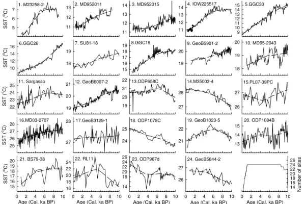
The temporal variations in a few of the reconstructed SST records from different por-tions of the North Atlantic display some differences (Fig. 2). For example, the SST in south of Iceland, offsouthwest Europe and offnorthwest Africa, and in the northwest Atlantic were warmest in the early Holocene (before 9.0 ka BP), and then underwent

5

step by step cooling during the last 10 ka. SST in the northeast Atlantic and offwest sub-tropical Africa slowly increased during the early Holocene. The peak warming usually occurred between 6–7.0 ka BP; since then the SST decreased. SST variations in the tropical Atlantic are somewhat less coherent. One SST record (site 14) in the western tropical Atlantic showed a rising trend whereas another record (site 15) nearby

10

showed a decreasing trend between 9–6 ka BP followed by increasing trend. Similar trend reversals (site 18 vs. site 19, site 21 vs. site 22) are found in east tropical Atlantic and the Mediterranean Sea. Overall, long-term cooling trends are found in the middle and high latitude North Atlantic, with mixed cooling/warming trends in the tropical At-lantic Ocean and the Mediterrean Sea. These differences can largely be attributed to

15

the specific characteristics of regional and local SST variations. The EOF method can thus be employed to isolate the dominant modes of individual SST records.

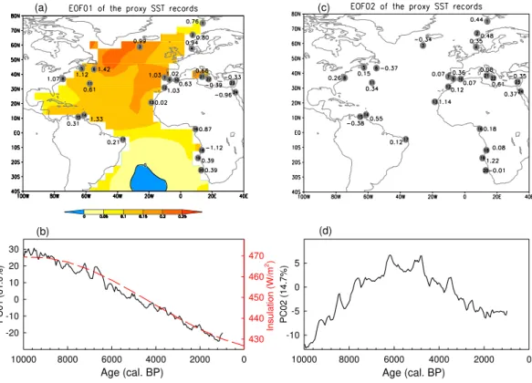
Spatial features in the North Atlantic Ocean are displayed by leading EOF modes of the Holocene SST variations. The first EOF (EOF01) accounts for 52.5% of the total SST variation during the Holocene (Fig. 3a), and shows a dominant and coherent SST

20

variation from the subtropical to the mid- and high-latitude North Atlantic. The tropical Atlantic showed mixed SST variations, and the eastern Mediterranean and the Red Sea showed SST anomalies opposite to that in the North Atlantic. High scores of EOF reflect positive loading from individual sites in the mid- and high-latitude Atlantic Ocean, whereas the scores in the tropical and low latitude are relatively small. The temporal

25

(8)

CPD

5, 2465–2496, 2009

S. Feng et al.

Tables Figures

◭ ◮

Back Close

Full Screen / Esc

suggests that the SST in the North Atlantic Ocean have been primarily decreasing over the last 10 ka, a result also indicated in previous studies using only alkenone-based SST reconstructions (Marchal et al., 2002; Kim et al., 2004, 2007). This cooling trend can best be explained by decreasing boreal summer insolation during the Holocene as suggested in Berger and Loutre (1991) and Lorenz et al. (2006) (Fig. 3b).

5

The second EOF (EOF02) explains 15.9% of the total variance. Because the EOFs are orthogonal to each other, the EOF02 describes the second largest SST variability unrelated to the EOF01. The spatial distribution (Fig. 3c) shows a less coherent pattern than EOF01, with high loading in the northeast Atlantic and the subtropical coast of Africa. The PC02 shows a pattern of progressively increasing scores to a maximum

10

at 6.2 ka BP followed by steady decline, indicating that the SST is increasing from the early to middle Holocene, and decreasing since then (Fig. 3d). This delayed Holocene warming was also identified in northeast North America, including Quebec and the Labrador Sea, and is likely related to the impact of Laurentide Ice sheets (Kaufman et al., 2004). This mode is much less important than the SST variability associated

15

with EOF01, however, explaining only 15.9% of the variance in contrast to more than three times as much (52.5%) explained by EOF01. The remaining EOFs account for less than 7.5% of the total variance and are not considered further as they essentially represent noise in the system.

In order to understand the atmospheric circulations related to the Holocene SST

20

patterns, we look for analogous SST patterns during the instrumental period. This procedure was previously used to explore the physical processes of SST patterns and thereby understand observed SST changes in the context of the Holocene (Rimbu et al., 2003; Kim et al., 2007). Because EOF01 is by far the dominant SST mode, the following analysis is focused on EOF01 and its instrumental analog.

25

(9)

CPD

5, 2465–2496, 2009

S. Feng et al.

Tables Figures

◭ ◮

Back Close

Full Screen / Esc

variations in the South Atlantic (Fig. 3a). Therefore, the EOF01 of Holocene SST is very similar to the first EOF of the observed SST related to the AMO, except that the Holocene SST contains variations on longer time scales. In other words, Figs. 2 and 3a, b suggested that the SSTs in the North Atlantic Ocean are warm during the early Holocene. These warm SST anomalies resemble the observed basin-wide warm

5

SST anomalies during the AMO warm phases. Following the cooling trend during the Holocene (Fig. 3b), the SST in the North Atlantic cools down. During the late Holocene the North Atlantic has cold anomalies that resemble the observed basin-wide cold SST anomalies during the AMO cold phases. The similarity of the SST patterns shown in Fig. 3a clearly depicts an AMO-like SST variation in the North Atlantic basin on

centen-10

nial and longer timescales during the Holocene. Because the EOF01 largely resembles the insolation forcing as seen in the climate models (e.g. Lorenz et al., 2006; Laepple and Lohmann, 2009), the AMO-like pattern is likely the regional manifestation of the orbital forcing in the North Atlantic Ocean. Lorenz et al. (2006) in their modeling study suggested that, when forced by orbital insolation changes during the Holocene, the

15

model could simulate a basin-wide cooling in the North Atlantic, a pattern that resem-bles the EOF01. The model, however, also simulated cooling trend over most of the Northern Hemisphere poleward of 30◦_{N, a result inconsistent with the warming trend}

revealed by the proxy records in the eastern North Pacific Ocean (Kim et al., 2004; Lorenz et al., 2006). This out-of-phase relationship between SST in the North Atlantic

20

and the North Pacific is also reproduced by long-term simulations made using a fully coupled model (Kim et al., 2004). Therefore, the long-term SST variations in the North Atlantic (the AMO-like pattern) and North Pacific Ocean during the Holocene were likely also influenced by other factors, including internal climate variability due to long-term fluctuations in the MOC.

25

(10)

CPD

5, 2465–2496, 2009

S. Feng et al.

Tables Figures

◭ ◮

Back Close

Full Screen / Esc

variability as shown in Fig. 3a. These results add confidence in the robustness of the AMO-like pattern of the Holocene SST variations in the North Atlantic Ocean. Be-cause temperatures during the early Holocene were strongly influenced by deglacia-tion (e.g. Kaufman et al., 2004), we also calculated EOFs for mid-to-late Holocene SST variations. The EOF01 based on the last 6.0 ka data is very similar to that shown in

5

Fig. 3a with the same signs (except sites 15 and 22, which are located in the tropi-cal Atlantic and the middle Mediterranean Sea), providing additional evidence that the basin-wide SST structure in the North Atlantic is persistent during the Holocene (see Table 1).

When the long-term SST trend at each site was removed (Fig. 2), the first two EOFs

10

still have the same patterns as the untrend results. The di_fferent simply that the EOF01 of the unfiltered SST records, the AMO-like pattern, now accounts much less of the detrended SST variance (14.1%), suggesting that the trend itself is important part of the AMO-like pattern during the Holocene.

Temporal variations of this AMO-like pattern are shown in Fig. 3b. The

centennial-15

scale variations are superimposed on a decreasing trend. After removing this trend, presumably due to orbital-induced summer insolation changes, by applying local weighted regression (Cleveland, 1979), the centennial timescale variations in PC01 clearly stand out (Fig. 4a). The multiple-taper spectrum (MTM, Mann and Lees, 1996) of this signal showed a significant peak around 700 years, which is about half of the

20

1450 year Bond cycles (Bond et al., 1997, 2001). The MTM also detected a weak peak around 2300 years (figure omitted). The 700 and 2300 year cycles in the SST were also found in previous studies (e.g. Rimbu et al., 2004). These centennial variations of PC01 appear closely coupled with variations of drift ice in the North Atlantic (Bond et al., 2001, see Fig. 4b), with warm (cold) temperatures associated with less (more) drift

25

(11)

CPD

5, 2465–2496, 2009

S. Feng et al.

Tables Figures

◭ ◮

Back Close

Full Screen / Esc

MOC (e.g. Dima and Lohmann, 2007). This was supported by Kim et al. (2007) that the Holocene SST variations in North Atlantic are closely related to variations of NADW. Therefore, Fig. 4 suggests that centennial SST variations of the AMO-like pattern may have been closely related to variations of the THC during the last 10 ka.

Figure 4a shows a distinct cold period that occurred from 8.0–8.6 ka BP; consistent

5

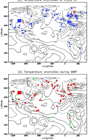
with the finding that broad, complex climate anomalies occurred during this time in-terval (Rohling and Palike, 2005), closely associated with the cold event that occurred around 8.2 ka BP (Alley et al., 1997). This cold event lasted for several hundred years and was first indentified in records from Greenland. Wiersma and Renssen (2006) summarized the published proxy data that record a cold event around 8.2 ka BP.

10

They found a clear concentration of records in the Northern Hemisphere especially for the North Atlantic. In this present study, in addition to the 63 proxy records sum-marized by Wiersma and Renssen (2006), 54 newly published temperature records around 8.2 ka BP on the North Atlantic Realm (130◦_W–50◦_{E, 40}◦_S–90◦_{N) also were}

analyzed. The locations and the inferred temperature variations of the proxy data

15

are shown on Fig. 5a, and the 54 new records are summarized in Table S1 (http: //www.clim-past-discuss.net/5/2465/2009/cpd-5-2465-2009-supplement.pdf). Among these 117 sites, only four in the North Atlantic region showed warm temperatures around 8.2 ka BP. All these four were based on pollen data and should describe the warm season or growing season temperatures. For the other 113 sites, their

tempera-20

tures were cold around 8.2 ka BP. The spatial distributions of these cold temepratures clearly resemble the observed temperature anomalies during the cold phase of AMO. As shown in Fig. 5a, there is a basin-wide cooling in the North Atlantic during AMO cold phases. The temperatures in the North America and Europe were also below nor-mal. Strong cooling (>₋_1.0◦_{C) occurred in Greenland, with weak cooling in the tropical}

25

Atlantic. Wiersma and Renssen (2006) also showed that a strong cooling (>₋7.4◦_C)

(12)

CPD

5, 2465–2496, 2009

S. Feng et al.

Tables Figures

◭ ◮

Back Close

Full Screen / Esc

Ocean are in a cold-phase AMO-like pattern at 8.2 ka BP, consistent with the cold event revealed by the PC01 (Fig. 4a).

Figure 4a also shows a warm period occurring roughly 1000 years ago, con-sistent with the medieval warm period (approximately 800–1300 AD) in Europe (Lamb et al., 1977). The published proxy data that span the MWP in the Atlantic

5

realm are summarized in Table S2 (http://www.clim-past-discuss.net/5/2465/2009/ cpd-5-2465-2009-supplement.pdf). A 50-year filter was applied to high resolution proxy records to isolate the low frequency variations. For a given site, if the low fre-quency temperature in the medieval times (800–1300 AD) was warmer (colder) than the temperature before 800 AD and after 1300 AD, the site was considered as

record-10

ing a warm (cold) period in the medieval times. Otherwise, the temperature in that site was considered to have no change. Figure 5b shows the spatial distribution of the medieval temperature anomalies in the North Atlantic. It is clear that the entire North Atlantic Ocean was warm during medieval times, so were in the North America and Europe. The regions with no change in temperature are found in the south tropical

15

Atlantic, and two sites in North America. The lack of change in temperature in south Colorado Plateau (Salzer and Kipfmueller, 2005) is possibly because the tree-ring data can not distinguish these low frequency temperature variations. There is also one site offthe California coast that showed cooling, a sign possibly related to a cooler tropical Pacific during medieval times (Kennett and Kennett, 2000; Feng et al., 2008).

Compari-20

son to the observed temperature patterns related to the warm phases of AMO (Fig. 5b) again suggests that the temperatures in the North Atlantic were also an AMO-like pat-tern during the medieval times. This patpat-tern is also consistent with the Holocene SST pattern revealed by the EOF01 (Figs. 3a and 4a).

In summary, the North Atlantic SST showed a basin-wide cooling around 8.2 ka BP

25

(13)

CPD

5, 2465–2496, 2009

S. Feng et al.

Tables Figures

◭ ◮

Back Close

Full Screen / Esc

Atlantic during the Holocene. A recent study of Bond et al. (2001) shows that tem-perature in North Atlantic realm has varied simultaneously on millennial and longer timescale (e.g. the Younger Dryas), further suggesting that an AMO-like signal is also likely a dominant SST mode in the North Atlantic on millennial timescales during recent geological times.

5

4 Discussions and conclusions

Our major result is that the dominant Holocene SST variations in the North Atlantic clearly resemble the observed AMO signal (a SST pattern). This result is different from some previous studies (Rimbu et al., 2003, 2004; Kim et al., 2004, 2007; Lorenz et al., 2006; Sachs, 2007) which argued that Holocene SST variations in the North Atlantic

10

resemble the North Atlantic Oscillation (NAO, which is fundamentally an atmospheric pattern). Rimbu et al. (2003) analyzed Holocene SST variations in the eastern North Atlantic, the Mediterranean Sea and northern Red Sea. Their first EOF showed an in-phase relationship between the variations of SST in the eastern North Atlantic and west Mediterranean Sea, and an out-of-phase relationship for SST variations in the

15

tropical western North Atlantic and the eastern Mediterranean Sea. To reveal the at-mospheric circulation related to the Holocene SST trend by looking for an analogous mode during the instrumental period, they defined an SST index by subtracting the averaged SST anomalies over the region dominant by positive Holocene SST trend (5–20◦_{N, 70–60}◦_{W for the western tropical North Atlantic and 20–40}◦_{N, 20–40}◦_{E for}

20

the eastern Mediterranean Sea) from the averaged SST anomalies over the region dominated by negative Holocene SST trend (30–70◦

N, 10◦

W – 20◦

E for the eastern North Atlantic). They found that the observed SLP pattern associated with their SST index was fairly similar to the SLP associated with the NAO, a result leading them to attribute Holocene SST variations in North Atlantic Ocean to long-term variations of the

25

(14)

CPD

5, 2465–2496, 2009

S. Feng et al.

Tables Figures

◭ ◮

Back Close

Full Screen / Esc

made similar arguments that Holocene SST variations in the North Atlantic resemble the observed NAO pattern.

Rimbu et al. (2003, 2004) in their analysis did not use SST records from the central and western middle latitude North Atlantic (e.g. sites 3, 5, 6, 8 and 11 in this study). In-cluding the SST records from those regions, however, demonstrates that the first EOF

5

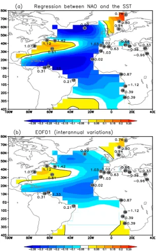
of Holocene SST does not resemble the overall NAO pattern. Figure 6a shows the re-gression between annual SST and annual NAO index for the period from 1870–2006. The SST pattern associated with NAO has an in-phase relationship between the west-ern tropical North Atlantic and the eastwest-ern middle North Atlantic and the Mediterranean Sea, a result that is not supported by the out-of-phase relationship between the two

re-10

gions revealed by Rimbu et al. (2003). Additionally, the results from Rimbu et al. (2003), Kim et al. (2004, 2007) and our Fig. 3a all show an in-phase relationship between the SST in the high-latitude eastern North Atlantic (e.g. our sites 1 and 2) and the middle latitude eastern North Atlantic (e.g. our sites 7, 9, 10 and 12). These in-phase relation-ships in the Holocene SST variations do not fit in the out-of-phase relationship typically

15

associated with the NAO (Fig. 6a). The SST records in the western middle-latitude North Atlantic (our sites 3, 5, 6, 8 and 11) are also discordant with the NAO-like SST pattern. Comparing the first EOF of the Holocene SST with the observed SST pattern associated with the NAO (Fig. 6a) and the AMO (Fig. 3a) suggests that the Holocene SST variations in the North Atlantic resemble an observed AMO-like pattern, not the

20

NAO-like pattern.

A possible reason for the mismatch between an NAO-like SST pattern and EOF01 of the Holocene SST in the North Atlantic is that the NAO signal is dominated by in-terannual variations. Figure 6b shows the first EOF of the observed (annual) SST on interannual timescales. It shows a tripole pattern in the North Atlantic,

resem-25

(15)

CPD

5, 2465–2496, 2009

S. Feng et al.

Tables Figures

◭ ◮

Back Close

Full Screen / Esc

decadal and longer timescales (Fig. 3a, and Fig. S1, http://www.clim-past-discuss.net/ 5/2465/2009/cpd-5-2465-2009-supplement.pdf). This result suggests that the underly-ing physical processes impactunderly-ing SST variations on interannual timescale are quite dif-ferent from those operating on decadal and longer timescales. Comparing Fig. 6a with Figs. 3a, 6b and the appending Fig. S1 (http://www.clim-past-discuss.net/5/2465/2009/

5

cpd-5-2465-2009-supplement.pdf) clearly suggests that the NAO-like pattern resem-bles SST variations on interannual timescales, but not the SST variations on decadal and longer timescales. We therefore suggest that it is more appropriate to compare Holocene SST variations with the AMO pattern (Fig. 3a) as the proxy SST records cannot resolve SST variations on interannual timescales.

10

Our interpretation is also supported by previous modeling studies. Kim et al. (2004) analyzed 2300-year simulations made with a fully coupled model. Their results sug-gested that surface temperatures in the eastern North Atlantic (30◦_{W – 10}◦_{E, 30 –}

70◦_{N) are significantly and positively correlated with the SST over the entire North}

Atlantic Ocean, except for the southwest tropical North Atlantic (where sites 14 and 15

15

are located), and the eastern Mediterranean and the Red Sea (where sites 22–24 are located; see their Fig. 6). Lorenz et al. (2006) analyzed modeled temperature varia-tions for the last 7.0 ka. When their model is forced by orbital insolation changes, the results showed a basin-wide cooling in annual and summer temperature for the North Atlantic. Additionally, their model results showed a weak warming in the southwest

20

tropical North Atlantic (where sites 14 and 15 are located) and the Red Sea (where site 24 are located). Those model results are quite similar to our results shown in Fig. 3a, supporting our conclusion that there are coherent and simultaneous Holocene SST variations over the North Atlantic Ocean. Therefore, even though Kim et al. (2004) and Lorenz et al. (2006) interpret their results as the NAO-like pattern, their model results

25

(16)

CPD

5, 2465–2496, 2009

S. Feng et al.

Tables Figures

◭ ◮

Back Close

Full Screen / Esc

differently for the atmosphere and the ocean.)

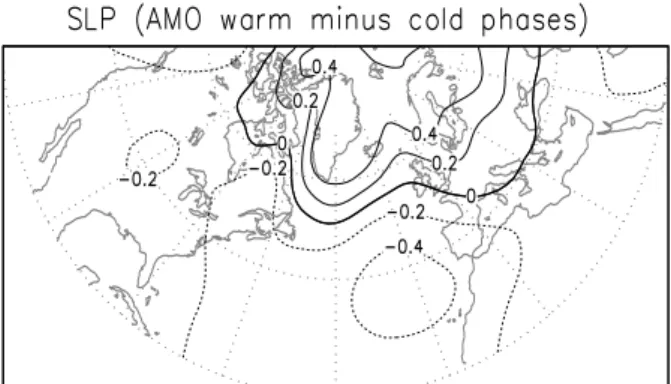
In order to find atmospheric circulations related to the AMO-like pattern, Fig. 7a shows composited SLP anomalies between the AMO warm and cold phases for the period 1870–2006. The SLP shows positive anomalies over the high latitude North Atlantic and the Arctic region, and negative anomalies over the middle latitude North

5

Atlantic region, a pattern very similar to the SLP associated with the NAO (Fig. 7b). Figure 7 suggests that during different phases of AMO, the North Atlantic is charac-terized by a quasi-monopolar SST pattern associated with a dipolar (NAO-like) SLP structure. A warm North Atlantic is related to SLP patterns similar to those of the negative phase of NAO, and vice versa. This connection between basin-wide SST

pat-10

terns and dipolar SLP patterns was also revealed by proxy SST and SLP data over the past 300 years and climate model simulations (Grosfeld et al., 2007; Roberson et al., 2000). Figure 7a is also very similar to the SLP anomalies associated with SST di_fferences between the eastern North Atlantic and the tropical western North Atlantic and eastern Mediterranean Sea (see Fig. 3b of Rimbu et al., 2003). The similarity

15

between Fig. 3b of Rimbu et al. (2003) and our Fig. 7 further suggests that different SST patterns in the North Atlantic are associated with similar dipolar SLP structures (NAO-like atmospheric pattern) in the Atlantic Ocean, and hence that simply interpret-ing Holocene SST variations in the North Atlantic as an NAO pattern is ambiguous. This ambiguous relationship between the NAO pattern and the SST is also supported

20

by climate model simulations. Rimbu et al. (2004) analyzed the relationship between the NAO and the surface temperature using a 2300 year simulations made with a fully coupled model. Their results suggested that on time scales greater than 100 years, the NAO pattern is associated with basin-wide positive SST anomalies in the North Atlantic Ocean. Whereas, on time scales shorter than 100 years, the NAO pattern

25

(17)

CPD

5, 2465–2496, 2009

S. Feng et al.

Tables Figures

◭ ◮

Back Close

Full Screen / Esc

suitable to interpret the EOF01 of Holocene SST as an AMO-like SST pattern.

Our Fig. 3a showed that SST variations in the southwest tropical North Atlantic (site 14) and the eastern Mediterranean and the Red Sea (sites 22–24) are out of phase with the basin-wide SST variations in the North Atlantic Ocean. Similar SST variation pattern was also obtained in climate models (e.g. Kim et al., 2004; Rimbu et

5

al., 2004; Lorenz et al., 2006). A possible physical mechanism is that the basin-wide SST variation in the North Atlantic causes a dipolar SLP variation (Fig. 7, Grosfeld et al., 2007; Roberson et al., 2000). The SLP could then interact with SST variations in the North Atlantic and the Mediterranean, helping induce the opposite SST variations in the eastern Mediterranean and the Red Sea (e.g. Hasanean, 2001).

10

Modeling studies suggest that strength of the AMO variability is strongly related to THC (Delworth and Mann, 2000; Knight et al., 2005). The AMO shift from warm to cold phase during the 1960s is also correlated with the observed Great Salinity Anomaly in the North Atlantic (Dickson et al., 1988). Previous results (Bond et al., 2001) and our Fig. 4 suggest that AMO-like SST patterns on centennial and millennial time scales

15

are closely related to variations in the THC. Additionally, the temperature anomalies on both ocean and land associated with the centennial and millennial SST changes in the North Atlantic are similar to those associated with the AMO during the instrumental period (Fig. 5, and Bond et al., 2001). All of these lines of evidence suggest that the multidecadal SST variations in the instrumental records, the centennial SST variations

20

in the Holocene, and the millennial SST variations in the geological times (e.g. the Younger Dryas) over the North Atlantic all share similar spatial extent and physical processes (e.g. the variations of THC).

In addition to basin-wide simultaneous SST variations in the North Atlantic, climate models also suggested a dipolar seesaw pattern between the North and South Atlantic

25

(18)

CPD

5, 2465–2496, 2009

S. Feng et al.

Tables Figures

◭ ◮

Back Close

Full Screen / Esc

records in Greenland and the Antarctica (Blunier et al., 1998). However, due to very few SST records available in the South Atlantic, the first EOF of the Holocene SST could not resolve the dipole pattern between the North and South Atlantic (Fig. 3a). Toledo et al. (2007) analyzed the SST variations (all based on δ18_{O of} _{G. ruber}_{) in}

three sites (CMU-14, ESP-08 and SAN-76, see also our Fig. 1) in the western tropical

5

South Atlantic during the last 30 ka. Two of their low-resolution SST records (ESP-08 and SAN-76) showed a warming trend during the last 10 ka, which is opposite to the cooling in the North Atlantic. In the eastern tropical south Atlantic, sites 19–20 showed a weak cooling, but site 18 showed a strong warming during the last 10 ka. Therefore, there are some indications that the South Atlantic is warming during the last 10 ka,

10

supporting the dipolar seesaw SST variations between the North and South Atlantic. However, more SST records in the middle and high latitude South Atlantic are needed to prove or disprove these seesaw SST variations during the Holocene.

Acknowledgements. We thank J. H. Kim and several others for making their proxy SST records

available to this study. This work was supported by USDA Cooperative Research Project

NEB-15

40-040, Office of Research at University of Nebraska-Lincoln project WBS 26-6238-0437-001, and NASA grant NNG06GE64G.

References

Allan, R. and Ansell, T.: A new globally complete monthly historical gridded mean sea level pressure dataset (HadSLP2): 1854–2004, J. Climate, 19, 5816–5842, 2006.

20

Alley, R. B., Mayewski, P. A., Sowers, T., Stuiver, M., Taylor, K. C., and Clark, P. U.: Holocene climatic instability – a prominent, widespread event 8200 yr ago, Geology, 25, 483–486, 1997.

Bard, E.: Climate shock: abrupt changes over millennial time scales, Physical Today, 55(12), 32–38, 2002.

25

(19)

CPD

5, 2465–2496, 2009

S. Feng et al.

Tables Figures

◭ ◮

Back Close

Full Screen / Esc

Blunier, T., Chappellaz, J., Schwander, J., Dallenbach, A., Stauffer, B., Stocker, T. F., Raynaud, D., Jouzel, J., Clausen, H. B., Hammer, C. U., and Johnsen, S. J.: Asynchrony of Antarctic and Greenland climate change during the last glacial period, Nature, 394, 739–743, 1998. Bond, G., Showers, W., Cheseby, M., Lotti, R., Almasi, P., DeMenocal, P., Priore, P., Cullen, H.,

Hajdas, I., and Bonani, G.: A pervasive millennial-scale cycle in North Atlantic Holocene and

5

glacial climates, Science, 278, 1257–1266, 1997.

Bond, G., Kromer, B., Beer, J., Muscheler, R., Evans, M. N., Showers, W., Hoffmann, S., Lotti-Bond, R., Hajdas, I., and Bonani, G.: Persistent solar influence on North Atlantic climate during the Holocene, Science, 294, 2130–2133, 2001.

Cleveland, W. S.: Robust locally weighted regression and smoothing scatterplots, J. Am. Stat.

10

Assoc., 74, 829–836, 1979.

Collin, M., Botzet, M., Carril, A. F., Drange, H., Jouzeau, A., Latif, M., Masina, S., Otteraa, O. H., Pohlmann, H., Sorteberg, A., Sutton, R., and Lerray, L.: Interannual to decadal climate predictability in the North Atlantic: A multimodel-ensemble study, J. Climate, 19, 1195–1203, 2006.

15

Delworth, T. L. and Mann, M. E.: Observed and simulated multidecadal variability in the North-ern Hemisphere, Clim. Dynam., 16, 661–676, 2000.

Delworth, T. L., Manabe, S., and Stouffer, R. J.: Multidecadal climate variability in the Greenland Sea and surrounding regions: A coupled model simulation, Geophys. Res. Lett., 24, 257– 260, 1997.

20

Dickson, R. R., Meincke, J., Malmberg, S. A., and Lee, A.: The “Great Salinity Anomaly” in the northern North Atlantic 1968–1982, Prog. Oceanogr., 20, 103–151, 1988.

Dima, M. and Lohmann, G.: A hemispheric meachanism for the Atlantic multidecadal oscilla-tion, J. Climate, 20, 2706–2719, 2007.

Enfield, D. B., Mestas-Nunez, A. M., and Trimble, P. J.: The Atlantic multidecadal oscillation

25

and its relation to rainfall and river flows in the continental U.S., Geophys. Res. Lett., 28, 2077–2080, 2001.

Farmer, E. C., deMenocal, P. B., and Marchitto, T. M.: Holocene and deglacial ocean temper-ature variability in the Benguela upwelling region: implications for low-latitude atmospheric circulation, Paleoceanography, 20, PA2018, doi:10.1029/2004PA001049, 2005.

30

(20)

CPD

5, 2465–2496, 2009

S. Feng et al.

Tables Figures

◭ ◮

Back Close

Full Screen / Esc

Feng, S. and Hu, Q.: How the North Atlantic Multidecadal Oscillation may have influenced the Indian summer monsoon during the past two millennia, Geophys. Res. Lett., 35, L01707, doi:10.1029/2007GL032484, 2008.

Feng, S., Oglesby, R. J., Rowe, C. M., Loope, D. B., and Hu, Q.: Atlantic and Pacific SST influences on Medieval drought in North America simulated by the community atmospheric

5

model, J. Geophys. Res., 113, D11101, doi:10.1029/2007JD009347, 2008.

Goldenberg, S. B., Landsea, C. W., Mestas-Nu ˜nez, A. M., and Gray, W. M.: The recent increase in Atlantic hurricane activity: Causes and implications, Science, 293, 474–479, 2001. Gray, S. T., Graumlich, L. J., Betancourt, J. L., and Pederson, G. T.: A tree-ring based

recon-struction of the Atlantic Multidecadal Oscillation since 1567 A.D., Geophys. Res. Lett., 31,

10

L12205, doi:10.1029/2004GL019932, 2004.

Grosfeld, K., Lohmann, G., Rimbu, N., Fraedrich, K., and Lunkeit, F.: Atmospheric multidecadal variations in the North Atlantic realm: proxy data, observations, and atmospheric circulation model studies, Clim. Past, 3, 39–50, 2007,

http://www.clim-past.net/3/39/2007/.

15

Hasanean, H. M.: Fluctuations of surface air temperature in the Eastern Mediterranean, Theor. Appl. Climatol., 68, 75–87, 2001.

Hu, Q. and Feng S.: Variation of North American summer monsoon regimes and the Atlantic multidecadal oscillation, J. Clim., 21, 2371–2383, 2008.

Kaufman, D. S., Ager, T. A., Anderson, N. J., Anderson, P. M., Andrews, J. T., Bartlein, P. J.,

20

Brubaker, L. B., Coats, L. L., Cwynar, L. C., Duvall, M. L., Dyke, A. S., Edwards, M. E., Eisner, W. R., Gajewski, K., Geirsdottir, A., Hu, F. S., Jennings, A. E., Kaplan, M. R., Kerwin, M. N., Lozhkin, A. V., MacDonald, G. M., Miller, G. H., Mock, C. J., Oswald, W. W., Otto-Bliesner, B. L., Porinchu, D. F., Ruhland, K., Smol, J. P., Steig, E. J., and Wolfe, B. B.: Holocene thermal maximum in the western Arctic (0 to 180◦_{W), Quaternary Sci. Rev., 23, 529–560, 2004.}

25

Keigwin, L. D.: The little ice age and medieval warm period in the Sargasso Sea, Science, 274, 1504–1508, 1996.

Kennett, D. J. and Kennett, J. P.: Competitive and cooperative responses to climatic instability in coastal Southern California, American Antiquity, 65, 379–395, 2000.

Kerr, R. A.: A North Atlantic climate pacemaker for the centuries, Science, 288, 1984–1986,

30

(21)

CPD

5, 2465–2496, 2009

S. Feng et al.

Tables Figures

◭ ◮

Back Close

Full Screen / Esc

Kim, J. H., Rimbu, N., Lorenz, S. J., Lohmann, G., Nam, S.-I., Schouten, S., Ruhlemann, C., and Schneider, R. R.: North Pacific and North Atlantic sea-surface temperature variability during the Holocene, Quaternary Sci. Rev., 23, 2141–2154, 2004.

Kim, J.-H. and Schneider, R.: GHOST global metadata compilation of sediment cores and references for alkenone-derived 10ka sea-surface temperature records, Department of

Geo-5

sciences, Bremen University, doi:10.1594/PANGAEA.425273, 2006.

Kim, J. H, Meggers, H., Rimbu, N., Lohmann, G., Freudenthal, T., Muller, P. J., and Schneider, R. R.: Impacts of the North Atlantic gyre circulation on Holocene climate offnorthwest Africa, Geology, 35, 387–390, 2007.

Knight, J. R., Allan, R. J., Folland, C. K., Vellinga, M., and Mann, M. E.: A signature of persistent

10

natural thermohaline circulation cycles in observed climate, Geophys. Res. Lett., 32, L20708, doi:10.1029/2005GL024233, 2005.

Knight, J. R., Folland, C. K., and Scaife, A. A.: Climate impacts of the Atlantic Multidecadal Oscillation, Geophys. Res. Lett., 33, L17706, doi:10.1029/2006GL026242, 2006.

Laepple, T. and Lohmann, G.: Seasonal cycle at template for climate variability on astronomical

15

timescales, Paleoceanography, 24, PA4201, doi:10.1029/2008PA001674, 2009. Lamb, H. H.: Climate present, past and future (v.2), Methuen and Co Ltd, London, 1977. Lea, D. W., Pak, D. K., Peterson, L. C., and Hughen, K. A.: Synchroneity of tropical and

high-latitude Atlantic temperatures over the last glacial termination, Science, 301, 1361–1364, 2003.

20

Lorenz, J. S., Kim, J.-H., Rimbu, N., Schneider, R. R., and Lohmann, G.: Orbitally-driven insolation forcing on Holocene climate trends: Evidence from alkenone data and climate modeling, Paleoceanography, 21, PA1002, doi:10.1029/2005PA001152, 2006.

Lu, R., Dong, B., and Ding, H.: Impact of the Atlantic multidecadal Oscillation on the Asian summer monsoon, Geophys. Res. Lett., 33, L24701, doi:10.1029/2006GL027655, 2006.

25

Mann, M. E. and Lees, H. M.: Robust estimation of background noise and signal detection in climate time series, Climatic Change, 33, 409–445, 1996.

Marchal, O., Cacho, I., Stocker, T. F., et al.: Apparent long-term cooling of the sea surface in the Northeast Atlantic and Mediterranean during the Holocene, Quaternary Sci. Rev., 21, 455–483, 2002.

(22)

CPD

5, 2465–2496, 2009

S. Feng et al.

Tables Figures

◭ ◮

Back Close

Full Screen / Esc

McCabe, G. J., Palecki, M. A., and Betancourt, J. L.: Pacific and Atlantic Ocean influences on multidecadal drought frequency in the United States, P. Natl. Acad. Sci. USA, 101, 4136– 4041, 2004.

New, M., Hulme, M., and Jones, P. D.: Representing twentiethcentury space–time climate variability, Part II: Development of 1901–96 monthly grids of terrestrial surface climate, J.

5

Clim., 13, 2217–2238, 2000.

Oppo, D. W., McManus, J. F., and Cullen, J. L.: Deepwater variability in the Holocene epoch, Nature, 422, 277–278, 2003.

Rayner, N. A., Parker, D. E., Horton, E. B., Folland, C. K., Alexander, L. V., Rowell, D. P., Kent, E. C., and Kaplan, A.: Global analyses of sea surface temperature, sea ice, and

10

night marine air temperature since the late nineteenth century, J. Geophys. Res., 108, 4407, doi:10.1029/2002JD002670, 2003.

Rimbu, N., Lohmann, G., Kim, J. H., Arz, H. W., and Schneider, R.: Arctic/North Atlantic Os-cillation signature in Holocene sea surface temperature trends as obtained from alkenone data, Geophys. Res. Lett., 30, 1280, doi:10.1029/2002GL016570, 2003.

15

Rimbu, N., Lohmann, G., Lorenz, S. J., Kim, J. H., and Schneider R. R.: Holocene climate variability as derived from alkenone sea surface temperature and coupled ocean-atmosphere model experiments, Clim. Dynam., 23, 215–227, 2004.

Robertson, A. W., Mechoso, C. R., and Kim, Y.-J.: The influence of Atlantic sea surface tem-perature anomalies on the North Atlantic oscillation, J. Clim., 13, 122–138, 2000.

20

Rohling, E. J. and Palike, H.: Centennial-scale climate cooling with a sudden cold event around 8,200 years ago, Nature, 434, 975–979, 2005.

Sachs, J. P.: Cooling of Northwest Atlantic slope waters during the Holocene, Geophys. Res. Lett., 34, L03609, doi:10.1029/2006GL028495, 2007.

Salzer, M. W. and Kipfmueller, K. F.: Reconstructed Temperature and Precipitation on a

Millen-25

nial Timescale from Tree-Rings in the Southern Colorado Plateau U.S.A., Climatic Change, 70, 465–487, 2005.

Schlesinger, M. E. and Ramankutty, N.: An oscillation in the global climate system of period 65–70 years, Nature, 367, 723–726, 1994.

Sutton, R. T. and Hodson, D. L. R.: Climate response to basin-scale warming and cooling for

30

the North Atlantic Ocean, J. Clim., 20, 891–907, 2007.

(23)

CPD

5, 2465–2496, 2009

S. Feng et al.

Tables Figures

◭ ◮

Back Close

Full Screen / Esc

von Storch, H. and Zwiers, F. W.: Statistical Analysis in climate research, Cambridge University Press, 1999.

Wang, C., Enfield, D. B., Lee, S.-K., and Landsea, C. W.: Influences of the Atlantic warm pool on Western Hemisphere summer rainfall and Atlantic hurricanes, J. Clim., 19, 3011–3028, 2006.

5

Wang, C., Lee, S., and Enfield, D. B.: Atlantic Warm Pool acting as a link between Atlantic multidecadal oscillation and Atlantic tropical cyclone activity, Geochem. Geophy. Geosy., 9, Q05V03, doi:1029/2007GC001809, 2008.

Weldeab, S., Schneider, R. R., and Kolling, M.: Deglacial sea surface temperature and salinity increase in the western tropical Atlantic in synchrony with high latitude climate instabilities,

10

Earth Planet. Sci. Lett., 241, 699–706, 2006.

Weldeab, S., Lea, D. W., Schneider, R. R., and Adnersen, N.: 155,000 years of West African monsoon and Ocean thermal evolution, Science, 316, 1303–1307, 2007.

Wiersma, A. P. and Renssen, H.: Model-data comparison for the 8.2 ka BP event: confirmation of a forcing mechanism by catastrophic drainage of Laurentide Lakes, Quaternary Sci. Rev.,

15

25, 63–88, 2006.

Zhang, R. and Delworth, T. L.: Impact of Atlantic multidecadal oscillations on India/Sahel rain-fall and Atlantic hurricanes, Geophys. Res. Lett., 33, L17712, doi:10.1029/2006GL026267, 2006.

Zhang, R., Delworth, T. L., and Held, I. M.: Can the Atlantic Ocean drive the observed

mul-20

(24)

CPD

5, 2465–2496, 2009

S. Feng et al.

Tables Figures

◭ ◮

Back Close

Full Screen / Esc

Printer-friendly Version Interactive Discussion Table 1.Summary of proxy SST records used in this study. The numbers indicate sites marked in Fig. 1. Superscript

“a” indicates SST records that began prior to 10 ka BP but only the SST values in recent 10 ka were used, and “b” indicates the missing SST records in IOW225517 during 0.45–1.83 ka BP were estimated using SST in Marine core IOW225514 via linear regression (data from Kim and Schneider, 2006). For site 11, the SST during the last 10 ka is reconstructed based on the regression betweenδ18O andδ18O-based SST construction during the last 3.0 ka. The 6th column shows the eigenvector value of EOF01 based on the 24 SST records and the subsets of 19 alkenone records (second number in the parenthesis) and 5 non-alkenone records (first number in the parenthesis). The 7th column is same as the 6th column but for last 6 ka.

No. Site and location Proxy Mean Data range EOF01 EOF01 Date sources type (min. to max.) (ka B.P.) (last 10 ka) (last 6 ka)

resolution (years)

North Atlantic

1 M23258-2 Alkenone 193 1.0–9.09 0.76 0.87 Kim and Schneider

75.00◦_{N 13.97}◦_E _(119–349) _{(–, 0.76)} _{(–, 0.88)} ₍₂₀₀₆₎

2 MD952011 Alkenone 64 0.51–8.39 0.80 0.87 Kim and Schneider

66.97◦_{N 7.63}◦_E _(4–266) _{(–, 0.80)} _{(–, 0.87)} ₍₂₀₀₆₎

3 MD952015 Alkenone 78 0.69–10.00a 0.99 0.33 Kim and Schneider

58.76◦_{N 25.96}◦_W _(25–254) _{(–, 1.00)} _{(–, 0.34)} ₍₂₀₀₆₎

4 IOW225517 Alkenone 77 0.45b–10.0a 0.94 1.00 Kim and Schneider

57.67◦_{N 7.09}◦_E _(8–271) _{(–, 0.94)} _{(–, 1.01)} ₍₂₀₀₆₎

5 OCE326-GGC30 Alkenone 75 0.13–10.0a 1.12 1.20 Sachs

43.89◦_{N 62.60}◦_W _(0–250) _{(–, 1.11)} _{(–, 1.20)} ₍₂₀₀₇₎

6 OCE326-GGC26 Alkenone 110 0.10–10.0a 1.42 1.14 ) Sachs

43.48◦_{N 54.87}◦_W _(0–260) _{(–, 1.43)} _{(–, 1.15)} ₍₂₀₀₇₎

7 SU81-18 Alkenone 321 0.0–10.0a 1.03 0.82 Bard

37.77◦_{N 10.18}◦_W _{(226–426 )} _{(–, 1.03)} _{(–, 0.83)} ₍₂₀₀₂₎

8 Ch07-98-GGC19 Alkenone 56 0.52–10.0a 1.07 1.08 Sachs

36.87◦_{N 74.57}◦_W _0–90) _{(–, 1.06)} _{(–, 1.06)} ₍₂₀₀₇₎

9 GeoB5901-2 Alkenone 33 1.13–9.92 1.02 0.42 Kim and Schneider

36.38◦_{N 7.07}◦_W _(4–317) _{(–, 1.03)} _{(–, 0.45)} ₍₂₀₀₆₎

10 MD952043 Alkenone 109 1.01–10.0a 0.63 0.50 Kim and Schneider

36.14◦_{N 2.62}◦_W _(49–223) _{(–, 0.64)} _{(–, 0.53)} ₍₂₀₀₆₎

11 Sargasso Sea δ18O 126 0.02–10.0a 0.61 0.60 Keiwign

(25)

CPD

5, 2465–2496, 2009

S. Feng et al.

Tables Figures

◭ ◮

Back Close

Full Screen / Esc

Printer-friendly Version Interactive Discussion Table 1.Continued.

No. Site and location Proxy Mean Data range EOF01 EOF01 Date sources type (min. to max.) (ka B.P.) (last 10 ka) (last 6 ka)

resolution (years)

North Atlantic

12 GeoB6007-2 Alkenone 29 0.00–9.99 1.03 0.95 Kim et al.

30.85◦_{N 10.27}◦_W _(10–50) _{(–, 1.04)} _{(–, 0.96)} ₍₂₀₀₇₎

Tropical Atlantic

13 ODP658c Alkenone 101 0.07–10.0a 0.02 0.68 Kim and Schneider

20.75◦_{N 18.58}◦_W _(27–370) _(–,

−0.03) (–, 0.69) (2006)

14 M35003-4 Alkenone 273 0.00–10.0a −1.33 −0.66 Kim and Schneider

12.08◦_{N 61.25}◦_W _(150–620) _(–,

−1.34) (–,−0.67) (2006)

15 PL07-39PC Mg/Ca 203 0.30–10.0a 0.31 −0.61 Lea et al.

10.70◦_{N 64.94}◦_W _(81–483) _{(0.31, –)} ₍

−0.70, –) (2003)

16 MD03-2707 Mg/Ca 40 0.36–10.0a 0.87 0.76 Weldeab et al.

2.50◦_{N 9.39}◦_E _(30–130) _{(0.81, –)} _{(0.77, –)} ₍₂₀₀₇₎

17 GeoB3129-1 Mg/Ca 202 0.17–10.0a 0.21 0.04 Weldeab et al.

4.61◦_{S 36.64}◦_W _(60–440) _{(0.46, –)} _{(0.01, –)} ₍₂₀₀₆₎

18 ODP1078C Alkenone 216 0.02–10.0a −1.12 −0.95 Kim and Schneider

11.92◦_{S 13.40}◦_E _(82–386) _(–,

−1.11) (–,−0.95) (2006)

19 GeoB1025-5 Alkenone 178 0.28–10.0a 0.39 1.19 Kim and Schneider

17.16◦_{S 11.01}◦_E _(72–297) _{(–, 0.36)} _{(–, 1.18)} ₍₂₀₀₆₎

20 ODP1084B Mg/Ca 105 0.0–10.0a 0.39 0.73 Farmer et al.

25.51◦_{S 13.03}◦_E _(51–220) _{(0.50, –)} _{(0.79, –)} ₍₂₀₀₅₎

Mediterranean and Red Sea

21 BS79-38 Alkenone 299 0.87–10.0a 0.66 0.53 Kim and Schneider

38.41◦_{N 13.58}◦_E _(98–520) _{(–, 0.65)} _{(–, 0.51)} ₍₂₀₀₆₎

22 RL11 Alkenone 256 0.15–10.0a −0.39 0.63 Kim and Schneider

36.75◦_{N 17.72}◦_E _(105–804) _(–,

−0.40) (–, 0.64) (2006)

23 ODP967d Alkenone 233 0.20–10.0a −0.33 −0.70 Kim and Schneider

34.07◦_{N 32.73}◦_E _(89–793) _(–,

−0.32) (–,−0.68) (2006)

24 GeoB5844-2 Alkenone 293 0.81–10.0a −0.96 −0.25 Kim and Schneider

27.71◦_{N 34.68}◦_E _(151–453) _(–,

(26)

CPD

5, 2465–2496, 2009

S. Feng et al.

Tables Figures

◭ ◮

Back Close

Full Screen / Esc

Printer-friendly Version Interactive Discussion Fig. 1. Spatial distribution of the proxy SST records used in this study. The (numbered) gray

(27)

CPD

5, 2465–2496, 2009

S. Feng et al.

Title Page Abstract Introduction Conclusions References Tables Figures ◭ ◮ ◭ ◮ Back Close

Full Screen / Esc

Printer-friendly Version Interactive Discussion 1. M23258-2 S S T ( oC ) 5 6 7 2. MD952011 11 12

13 3. MD952015

11 12 13

14 4. IOW225517

11 12 13 14 7. SU81-18 18 19 9. GeoB5901-2 19 20 10. MD95-2043 18 19 20 11. Sargasso S S T ( oC ) 22 23 24

25 12. GeoB6007-2

19 20 21 13.ODP658C 19 20 21 22 _14.M35003-4 27 28 15.PL07-39PC 26 27 16.MD03-2707 S S T ( oC ) 25 26 27 28 17.GeoB3129-1 27 28 8.GGC19 15 16 17 18 19 6.GGC26 S S T ( oC ) 10 12 14 16 5.GGC30 9 10 11 12 13 14 15 18. ODP1078C 24 25 19. GeoB1023-5 21 22 20. ODP1084B 13 14 15 21. BS79-38

Age (Cal. ka BP)

0 2 4 6 8 10

S S T ( oC ) 15 16 17 18 19

20 22. RL11

Age (Cal. ka BP)

0 2 4 6 8 10 16

18 20 22

24 23. ODP967d

Age (Cal. ka BP)

0 2 4 6 8 10 14 16 18 20 22 24

26 _{24. GeoB5844-2}

Age (Cal. ka BP)

0 2 4 6 8 10 26

27

Age (Cal. ka BP)

0 2 4 6 8 10

N u m b e r o f s it e s 14 16 18 20 22 24 26

(28)

CPD

5, 2465–2496, 2009

S. Feng et al.

Title Page Abstract Introduction Conclusions References Tables Figures ◭ ◮ ◭ ◮ Back Close

Full Screen / Esc

Age (cal. BP)

0 2000 4000 6000 8000 10000 P C 0 1 ( 6 1 .0 % ) -20 -10 0 10 20 30 In s u la ti o n ( W /m 2) 430 440 450 460 470 (a) (b) (c) (d)

Age (cal. BP)

0 2000 4000 6000 8000 10000 P C 0 2 ( 1 4 .7 % ) -10 -5 0 5

Fig. 3. EOF results of the proxy SST records. (a) Spatial distribution of the first EOF. The (numbered) gray dots show the 24 sites where proxy SST records were obtained (see Table 1 for site details). The value by each site is the eigenvector of the first EOF of the proxy SST record. (For illustration purposes, shading shows the first EOF of the observed SST in the North Atlantic Ocean, essentially the AMO pattern as defined from observations).(b)PC01 of the 24 proxy SST records (thick line) and July insolation at 65◦_{N during the Holocene (dashed}

(29)

CPD

5, 2465–2496, 2009

S. Feng et al.

Tables Figures

◭ ◮

Back Close

Full Screen / Esc

(a)

(b)

R

e

s

id

u

a

l

o

f

P

C

0

1

-6 -4 -2 0 2 4 6

Age (cal. BP)

0 2000

4000 6000

8000 10000

D

ri

ft

i

c

e

i

n

d

ic

e

s

0

5

10

15

(30)

CPD

5, 2465–2496, 2009

S. Feng et al.

Tables Figures

◭ ◮

Back Close

Full Screen / Esc

Printer-friendly Version Interactive Discussion Fig. 5. (a)Upper panel: spatial distribution of the proxy data that recorded temperature changes around 8.2 ka BP.

(31)

CPD

5, 2465–2496, 2009

S. Feng et al.

Tables Figures

◭ ◮

Back Close

Full Screen / Esc

Printer-friendly Version Interactive Discussion Fig. 6.(a)Regression between the annual NAO index and annual SST in the North Atlantic over the period of 1870–

(32)